Sensor Data Compression Using Bounded Error Piecewise Linear Approximation with Resolution Reduction


1
Department of Information Management, Tunghai University, Taichung 40704, Taiwan
2
Department of Computer Science and Information Engineering, National Taiwan University, Taipei 10617, Taiwan
3
Department of Computer Science, Tunghai University, Taichung 40704, Taiwan
*
Author to whom correspondence should be addressed.
Energies 2019, 12(13), 2523; https://doi.org/10.3390/en12132523
Submission received: 27 April 2019
/
Revised: 15 June 2019
/
Accepted: 17 June 2019
/
Published: 30 June 2019
(This article belongs to the Special Issue Smart Management Energy Systems in Industry 4.0)
Abstract
:Smart production as one of the key issues for the world to advance toward Industry 4.0 has been a research focus in recent years. In a smart factory, hundreds or even thousands of sensors and smart devices are often deployed to enhance product quality. Generally, sensor data provides abundant information for artificial intelligence (AI) engines to make decisions for these smart devices to collect more data or activate some required activities. However, this also consumes a lot of energy to transmit the sensor data via networks and store them in data centers. Data compression is a common approach to reduce the sensor data size so as to lower transmission energies. Literature indicates that many Bounded-Error Piecewise Linear Approximation (BEPLA) methods have been proposed to achieve this. Given an error bound, they make efforts on how to approximate to the original sensor data with fewer line segments. In this paper, we furthermore consider resolution reduction, which sets a new restriction on the position of line segment endpoints. Swing-RR (Resolution Reduction) is then proposed. It has O(1) complexity in both space and time per data record. In other words, Swing-RR is suitable for compressing sensor data, particularly when the volume of the data is huge. Our experimental results on real world datasets show that the size of compressed data is significantly reduced. The energy consumed follows. When using minimal resolution, Swing-RR has achieved the best compression ratios for all tested datasets. Consequently, fewer bits are transmitted through networks and less disk space is required to store the data in data centers, thus consuming less data transmission and storage power.
1. Introduction
Recently, Industry 4.0 has been commonly referred to as the fourth industrial revolution. It mainly focuses on manufacturing automation which is enabled by Internet of Things (IoT), big data, cloud computing, and artificial intelligence (AI) to enhance schedules and processes of production lines, aiming to reduce production costs, improve product quality, and shorten production time. Smart production is one of the key issues for the world to advance toward Industry 4.0. Automatic production optimization is also one of the methods to improve production throughputs and to quickly and flexibly respond to customer-oriented market. In a smart factory, hundreds or even thousands of sensors and smart devices are often deployed, e.g., for production line monitoring or product inspection. By analyzing collected sensor data, smart engines can make proper decisions, e.g., to stop the production line immediately when a severe anomaly is detected, to avoid producing defective products. As a result, these smart devices can adjust their actions dynamically and function effectively and efficiently to make this factory usually stay in its normal production stage. Many manufacturing issues have been explored in Industry 4.0 in recent years. For example, preventive maintenance [1] of equipment is to ensure that it is free from failure between one maintenance session and the next planned maintenance session. To achieve this, the equipment’s worn components are repaired or replaced in advance, even they are still workable now. It is shown that it could greatly enhance the resilience of the system by replacing a partial functional component with a fully functional one [2]. States of the system are continuously monitored to make sure that the system works normally. Condition data are analyzed to decide the right time for performing maintenance on the right components. However, the big data generated by sensors also consumes a lot of energy, including the corresponding data transmission from the sensors to data centers, and data storage in the data centers. Shehabi et al. in [3] reported that data centers in the U.S. consumed an estimated of 70 billion kW h in 2014. It was about 1.8% of total U.S. electricity consumption in that year and expectedly increases 4% from 2014 to 2020. Energy consumption in networking occupies a significant percentage of total energy consumption in cloud computing [4]. The increase of data volume and length aggravates the data storage and transmission burdens [5]. The best practices for saving power in data centers include reduction of storage disk space, and network port power consumption [3].
Basically, data compression is a common approach to reduce data size. For example, in a smart grid scenario, smart meter readings are first compressed in a distributed approach, and then classified and stored at a remote data center [5]. In general, compression ratios of lossless compression approaches are not high. Most of them follow Huffman coding [6,7,8,9,10]. On the other hand, there is no guarantee between the original data and compressed data by using lossy compression methods. Schemes learnt from image compression based on vector quantization, discrete cosine transform (DCT), wavelet transform (WT), and so on are adopted [11,12,13,14,15]. Three types of correlations hidden in the data—including temporal correlation, spatial correlation, and data correlation—are investigated for data compression. In [16], data correlation according to information theory are leveraged so that data occurred more frequently are encoded by shorter codes. Since sensor data are usually similar within a short period of time, many methods deal with temporal correlation [17,18,19,20,21]. Spatial correlation are explored when multiple sensors are located closely and the sensor data are very similar expectedly [19,20,21,22,23,24,25]. In [26], the three types of correlations are investigated, and errors between the original sensor data and compressed data are bounded to support data aggregation.
Data sensed periodically by sensors are essential time series, e.g., temperature, humidity, speed, direction, volumetric flow, pressure, concentration, etc. Bounded-error approximation to the original sensor data can retain a certain level of quality of the compressed data [27,28,29,30,31,32,33,34]. Literature indicates that many Bounded-Error Piecewise Linear Approximation (BEPLA) methods have been proposed—e.g., Swing filter [31], Slide filter [31], Cont-PLA [27], and mixed-PLA [34]—all of which focused on how to approximate to the original data with fewer line segments.
In this paper, we further consider resolution reduction when creating BEPLA. On selecting endpoint for BEPLA, resolution reduction sets a new restriction so that fewer bits are allowed to encode the endpoints of line segments. A variant method with Swing filter [31], named Swing-RR, is proposed. Swing-RR has optimal O(1) time and space complexities in processing data records. Using real world datasets, our experiment results show that although Swing-RR uses more line segments than those state-of-the-art methods, the size of sensor data are significantly reduced by resolution reduction, implying that the mean square errors between the original data and compressed data are also smaller. Of course, energy consumed for delivering and saving compressed data will be significantly lowered.
1.1. Bounded-Error Piecewise Linear Approximation (BEPLA)
Here, we first simply describe BEPLA and then define the problems to be solved in this paper.
1.1.1. Definition 1: Bounded-Error Approximation (BEA)
For a time series y(t) = (y1, y2, y3, …, yn), an approximation y’(t) = (y1′, y2′, y3′, …, yn’) to y(t) is bounded-error by a preassigned error bound ε when |yi − yi’| ≤ ε for all i = 1, 2, …, n. In this paper, yi’ is the approximated data point of data point yi.
In literature, many criteria have been utilized to assess the quality of an approximation against that of original time series. A criterion called p-norm of the errors between them, denoted by lp-error, is shown in Equation (1), which measures the distance between them. Commonly used lp-error are l1-error, l2-error, and l∞-error, which are shown in Equations (2)–(4), respectively. These distances are frequently employed in time series analyses. l1-error and l2-error are also called Manhattan distance and Euclidean distance, respectively. Since the whole series are taken into consideration, they are rarely used in online scenarios, in which every portion of the approximation has to be generated as soon as available. These two lp-error are considered as an average distance globally, rather than an instant distance locally. For an approximation that has a small l1-error and/or l2-error, there is no trivial bound on the error between any particular data point and its approximated data point.
Unlike l1-error and l2-error, l∞-error measures the largest error between any data point and its approximated. When l∞-error is bounded, loose bounds of l1-error and l2-error for any portion of the approximation can be easily derived. Also, for any line segment si with the length of m, l1-error and l2-error between si and y(t) are bounded by mε and , respectively.
1.1.2. Definition 2: Piecewise Linear Approximation (PLA)
PLA as a classic representation method is often used to describe two-dimensional data series, ((x1, y1), (x2, y2), …, (xn, yn)). A PLA to a data series consists of k (k ≤ n) continuous non-overlapping line segments (s1, s2, …, sk), in which si (1 ≤ i ≤ k) approximating to a portion of the original data is represented by two endpoints, i.e., (si.start.x, si.start.y) and (si.stop.x, si.stop.y). The length of si in x-axis is expressed as si.length = si.stop.x − si.start.x + 1.
PLA has many applications [35]. For example, in piecewise linear regression, the original data are divided into several segments, each of which is fitted by using linear regression. Note that linear regression tries to find the best line to approximate to the original data series, meanwhile minimizing l2-error. As mentioned above, when using PLA, there is no bound between any particular data point and its approximated data point.
When ((x1, y1), (x2, y2), …, (xn, yn)) is a time series sensed periodically, i.e., xi is the time tick i (1, 2, …, n), the series is represented as (y1, y2, …, yn) for short in this paper.
1.1.3. Definition 3: Bounded-Error Piecewise Linear Approximation (BEPLA)
Given time series y(t) = (y1, y2, …, yn) and preassigned error bound ε, BEPLA y’(t) = (s1, s2, …, sk), k ≤ n, is a PLA to y(t) and the l∞-error between y(t) and y’(t) is bounded by ε.
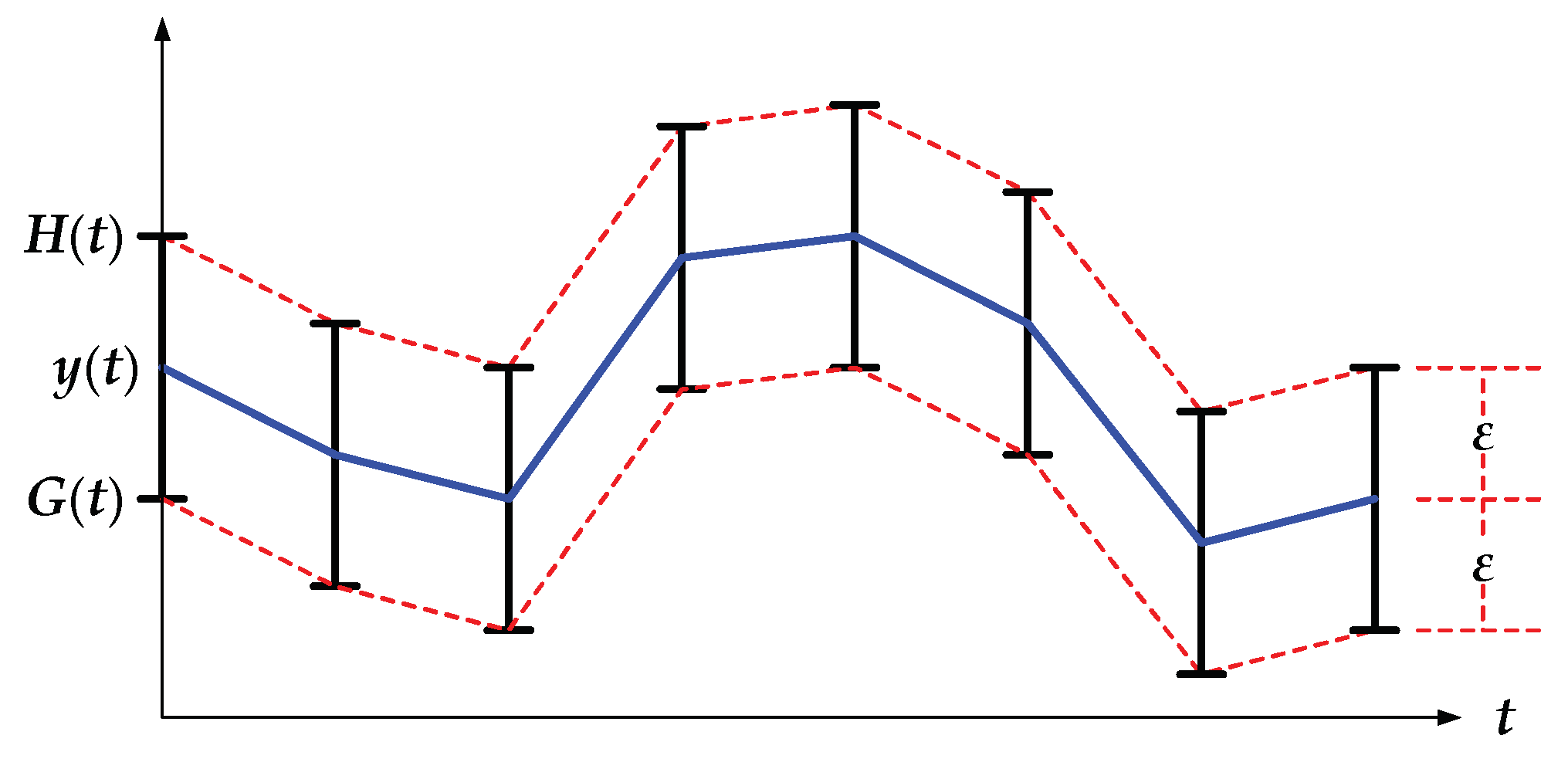
In recent years, BEPLA for sensor data have attracted researchers’ eyes once again [29,30,31,34]. As shown in Figure 1, given time series y(t) and preassigned maximal error ε, we can set upper bound H(t) and lower bound G(t) for y’(t), as listed in Equations (5) and (6), respectively.
H(t) = y(t) + ε
G(t) = y(t) − ε
Although the two εs in both Equations (5) and (6) are the same, they may be different in different applications.
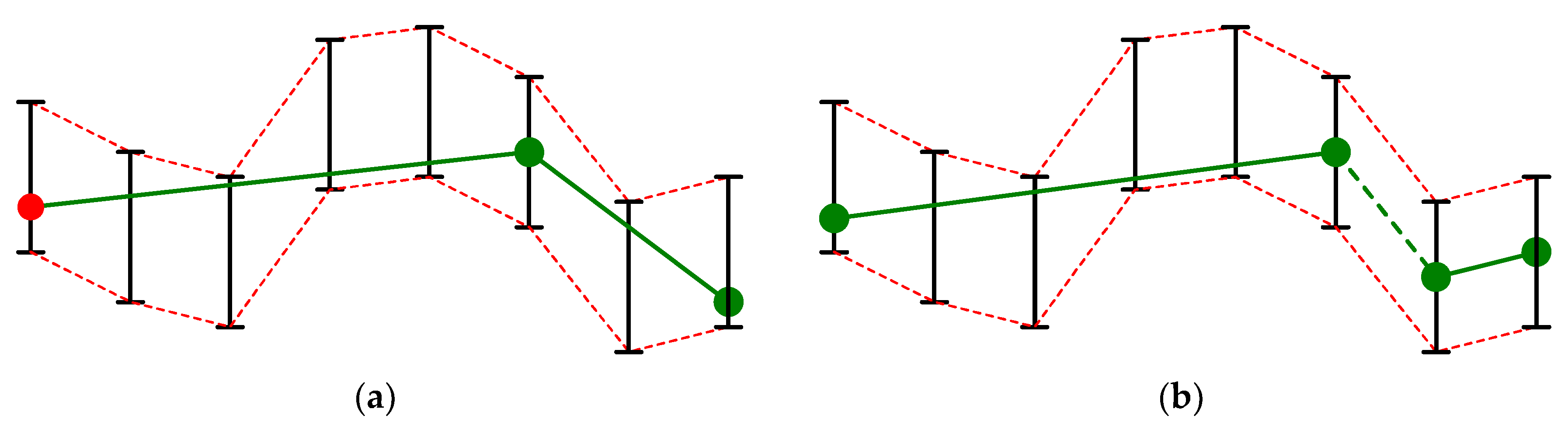
In fact, BEPLA y’(t) = (s1, s2, …, sk) is a PLA to y(t) and the l∞-error between y(t) and y’(t) is bounded by ε if and only if all points in all line segments are between G(t) and H(t). For any line segment si, the length of which is m, it is easy to prove that l1-error and l2-error between si and y(t) are bounded by mε and , respectively. As shown in Figure 2, there are two types of BEPLA, joint and disjoint. In joint BEPLA, consecutive line segments share an endpoint, i.e., si+1.start is actually si.stop (1 ≤ i < k), as shown in Figure 2a. In addition to the start point of the first line segment (i.e., s1.start), for each line segment, the stop point is recorded. Specifically, y’(t) is recorded as (s1.start.y, (s1.length, s1.stop.y), (s2.length, s2.stop.y), …, (sk.length, sk.stop.y)). Note that s1.start.x = 1, and si.stop.x = si+1.start.x = si.start.x + si.length.x − 1 for all is, 1 ≤ i < k. When the value of y is stored in p bits and the length of a line segment is stored in q bits, y’(t) is recorded in p + (p + q)k bits. Thus, compression ratio for joint BEPLA can be calculated by using Equation (7).
where n is the number of elements in the original time series y(t), and 32 is the number of bits used to represent yi in y(t), for all is. In disjoint BEPLA, a line segment si+1 does not have to start from the stop point of si (1 ≤ i < k). In practice, si+1 starts from the next time tick after the stop point of si, i.e., si+1.start.x = si.stop.x + 1 for all is, 1 ≤ i < k, as shown in Figure 2b. Since there are no shared endpoints between consecutive line segments, both start and stop points of a line segment need to be recorded. Specifically, y’(t) is recorded as ((s1.start.y, s1.length, s1.stop.y), (s2.start.y, s2.length, s2.stop.y), …, (sk.start.y, sk.length, sk.stop.y)). Note that s1.start.x = 1, and si.stop.x = si.start.x + si.length.x − 1 for all is, 1 ≤ i ≤ k. Thus, y’(t) is recorded in (2p + q)k bits. Compression ratio for disjoint BEPLA is calculated by using Equation (8).
In fact, there are k − 1 hidden line segments whose length is 1 time tick, as the dashed line segment shown in Figure 2b. They are (si.stop.y, 1, si+1.start.y) for all is, 1 ≤ i < k, and embedded in the representation of y’(t). In other words, there are actually 2k − 1 line segments. These hidden line segments are not explicitly recorded since they can be derived from the representation of disjoint BEPLA.
Many BEPLA algorithms have been so far proposed [27,28,29,30,31,32,33,34], trying to extend the line segments as long as possible and thus minimizing the number of line segments. In 2009, Elmeleegy et al. [31] reinvented Swing filter and Slide filter for joint and disjoint BEPLA, respectively. Swing filter is the simplest, but not optimal in terms of number of line segments. Its complexities on a data point in both time and space are O(1). In fact, Swing filter was presented by Gritzali and Papakonstantinou in 1983 [33]. An optimal joint BEPLA algorithm, referred to Cont-PLA in this paper, was introduced by Hakimi and Schmeichel in 1991 [27,28]. Slide filter is optimal in minimizing number of line segments. Actually, an optimal disjoint BEPLA algorithm was proposed by O’Rourke in 1991 [32]. Xie et al. [29] in 2014 improved the running time efficiency of Slide filter. Zhao et al. [30] in 2016 improved the efficiency of Swing filter based on [29]. Using convex hull and similar techniques, the amortized time complexity of both Cont-PLA and Slide filter on a data point are also O(1).
For data compression consideration, each line segment consumes p + q bits in joint BEPLA while 2p + q bits in disjoint BEPLA. Since disjoint BEPLA algorithms have higher freedom in selecting the start points of line segments, they usually use fewer line segments. As shown in [29], in terms of bits representing the resultant BEPLA, Cont-PLA, and Slide filter mutually outperformed each other on different datasets, and both achieved 15–25% superiority over swing filer in all datasets. In 2015, Luo et al. [34] introduced Mixed-PLA that uses both joint and disjoint line segments. The authors employed dynamic programming technique and showed that Mixed-PLA were roughly 15% better than Cont-PLA and Slide filter in terms of bits representing the resultant BEPLA.
1.2. BEPLA with Resolution Reduction
Here, we define the problems that BEPLA with resolution reduction may face.
As described above, the only requirement of a proper BEPLA is that all line segments must be between G(t) and H(t). In fact, even the x-coordinates of line segment endpoints are not restricted to be aligned with the time ticks, as a result, the x- and y-coordinates of line segment endpoints are real numbers, and stored as float point numbers, which are typically 32 bits long. If we set some restriction on position of line segment endpoints, we can use less number of bits to encode x- and y-coordinates of them.
In this paper, resolution reduction is further taken into consideration. In practice, error bounds (ε) typically range from 0.5% to 5% of the whole range of possible sensor data [29,31,34]. We note that before data compression, it can apply an extreme filter [36] to remove the influence of unfavorable data points. Therefore, 2ε is from 1% to 10%. If r bits are used to approximate to the data, the whole range of possible sensor data is then divided into 2r blocks, and the center of each block is coded accordingly, named coded data point in this paper. When the block size (1/2r) is smaller than 2ε, there must be at least ⌊ε2r+1⌋ coded data points between G(t) and H(t) at any particular time. Table 1 shows the minimal resolution (in bits), calculated by using Equation (9), for typical error bounds.
in which ⌈.⌉ is ceiling function. In other words, when r is larger than or equal to the minimal resolution for the preassigned error bound ε, for any particular data point y, there must be at least one coded data point y* such that the distance between y* and y is bounded by ε.
Minimal Resolution (ε) = ⌈−log2(ε) − 1⌉
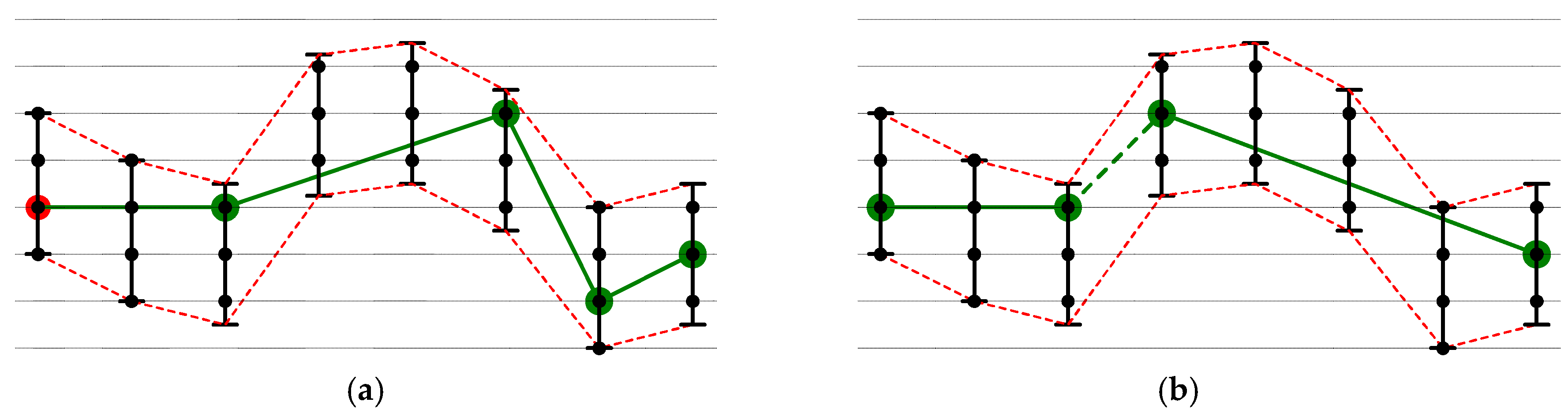
When resolution reduction is adopted by BEPLA algorithms, the endpoints of line segments must be all coded data points, as shown in Figure 3, where coded data points are depicted as black circles. We must note that in this configuration, it does not mean the approximated data points, except the start point and stop point, on a line segment are coded data points.
Apparently, adoption of resolution reduction by BEPLA puts a new restriction on endpoint selection for line segments. As shown in Figure 3a,b, the first line segments in both joint and disjoint BEPLA stop after three data points are examined. However, in Figure 2a,b, the first line segments in both joint and disjoint BEPLA stop after six data points are examined and their lengths in time are both five time ticks, implying that the adoption of resolution reduction might shorten the line segments used to approximate to the original time series, thus generating more line segments. Referring to Equations (7) and (8), even when the number of line segments (k) increases, we can reduce the size of BEPLA by using fewer bits (p and q bits) to represent the approximated data point and the length of a line segment. For example, when the error bound is set to 0.5% and minimal resolution is used, the y-coordinate of a line segment endpoint is stored in 7 bits rather than 32 bits. The reduction is significant for both Equations (7) and (8) and usually can compensate for the increase of k, i.e., the length of a BEPLA.
In this paper, the simplest method, Swing filter [31], is extended to take resolution reduction into consideration. To the best of the authors’ knowledge, Swing-RR is the first BEPLA algorithm that adopts resolution reduction.
Swing-RR generates disjoint BEPLA rather than joint BEPLA. Its time and space complexities are both O(1), the same as those of Swing filter. Hence, Swing-RR can be applied to be used by sensor networks, edge computing, and scenarios in which computing power and energy are limited. For real-time event detection and processing, i.e., line segments must be generated before a preassigned number of data points is sensed, the length of line segments can be bounded by a maximal delay in Swing-RR.
Real world datasets, the UCR time series classification archive [37], are used to investigate the performance of Swing-RR. Experiment results show that Swing-RR significantly outperforms Swing filter. The bits used to represent BEPLA generated by Swing-RR are only 20–35% of those produced by Swing filter for typical error bounds. Swing-RR generates more line segments than Swing filter. The lengths of its line segments in time are shorter, thus better fitting the original data. The mean square errors of BEPLA generated by Swing-RR is smaller than those produced by Swing filter.
2. Method
This section describes how to generate a BEPLA by Swing-RR.
Algorithm 1 shows the pseudocode of Swing-RR (). Given error bound ε, maximal delay delay, and resolution r bits in length, whenever a new data point d is sensed, d is processed by Swing-RR(d) and line segments are generated on the fly.
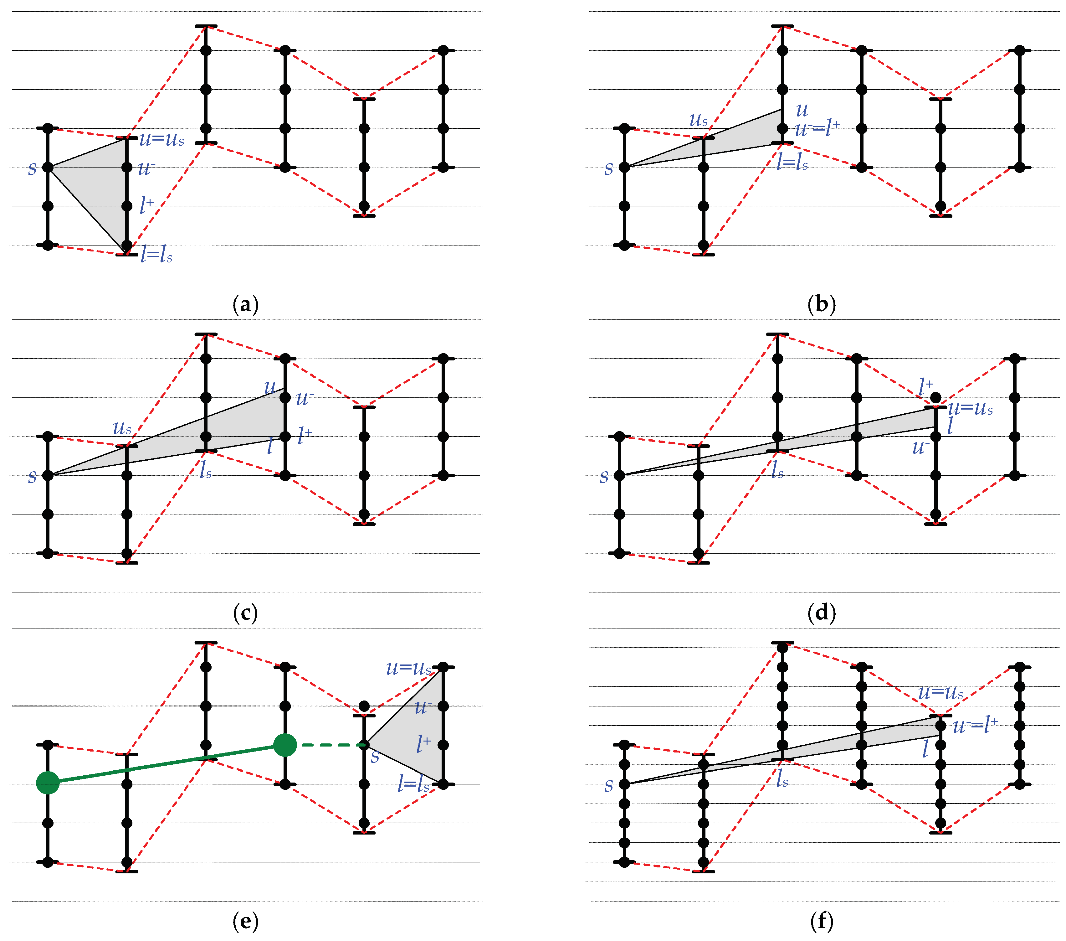
Similar to Swing filter, Swing-RR maintains a data structure for holding possible line segments. As shown in Figure 4, two auxiliary lines s→us and s→ls are maintained. The possible line segments for the current processing window must lie within s→us and s→ls. Both auxiliary lines start from the start point s of the current processing window.
| Algorithm 1: Swing-RR(d), given error bound ε, maximal delay delay, and resolution r bits in length |
| 1: segment.length++ // segment.length is initialized to −1 fora new window |
| 2: if (segment.length == 0) then // the first data point in this window |
| 3: segment.start s = picking up a coded data point between d + ε and d − ε; |
| 4: else if (segment.length == 1) then // the second data point in this window |
| 5: us = d + ε; ls = d − ε; |
| 6: check_range (); |
| 7: else if ((d + ε is below s→ls) or (d − ε is above s→us) |
| 8: {close this window; generate a line segment; initialize a new window;} |
| 9: else |
| 10: if (d + ε is below s→us) us = d + ε; // s→us swing down |
| 11: if (d − ε is above s→ls) ls = d − ε; // s→ls swing up |
| 12: check_range (); |
| 13: end if |
| 14: |
| 15: Function check_range () |
| 16: u = the point at d.t extended from s→us; |
| 17: l = the point at d.t extended from s→ls; |
| 18: u− = the largest coded data point smaller than or equal to u; |
| 19: l+ = the smallest coded data point larger than or equal to l; |
| 20: if (l+ ≤ u−) then // there exists at least one coded data point |
| 21: segment.stop = (l+ + u−)/2; |
| 22: if (segment.length ≥ delay) // Swing-RR is forced to output a line segment |
| 23: {close this window; generate a line segment; initialize a new window;} |
| 24: end if |
| 25: else // there exist no coded data points |
| 26: {close this window; generate a line segment; initialize a new window;} |
| 27: end if |
When a window is initialized, a coded data point in the bounded range of the first sensed data point is chosen, probably randomly (please refer to lines 2 and 3 of Algorithm 1 and Figure 4a). In this experiment, a coded data point nearest to the original data is chosen.
When the second data point d in this window is processed, two support points, us = d + ε and ls = d − ε, are initialized accordingly (please refer to lines 4~6 of Algorithm 1 and Figure 4b). The upper support point us bounds the maximal slope of possible line segments, i.e., s→us. The lower support point ls bounds the minimal slope of possible line segments, i.e., s→ls.
Similar to Swing filter, whenever a new data point d is sensed, the two support points, us and ls, are maintained according to the positions of d + ε and d − ε. s→us may swing down, and s→ls may swing up (please refer to lines 7~11).
If d + ε is below s→ls and thus s→us will swing down too much, a line segment is then generated. Also, if d − ε is above s→us and thus s→ls will swing up too much, a line segment is generated (please refer to lines 7~8). Otherwise, us and ls are maintained to update the range of possible line segments (please refer to lines 10 and 11). If d − ε is above s→ls, s→ls swings up by updating ls = d − ε, as shown in Figure 4a,b. If d + ε is below s→us, s→us swings down by updating us = d + ε, as shown in Figure 4c,d.
When resolution reduction is adopted, please see function check_range(), Swing-RR further checks to see whether there are coded data points between l and u, which are extended from s→ls and s→us, respectively. Specifically, Swing-RR calculates l+ and u− where l+ is the smallest coded data point larger than or equal to l, and u− is the largest coded data point smaller than or equal to u, as shown in Figure 4b–d. We note that s, l+, and u− must be coded data points, while us, ls, u, and l are not restricted to be coded data points. When l+ is smaller than or equal to u−, there must be at least one data point between l and u. A coded data point between l+ and u− is chosen as the stop point of a line segment candidate for this window. Swing-RR adopts the middle coded data point between l+, and u− (please refer to line 21). On the other hand, when l+ is larger than u−, there is no coded data point between l and u, as shown in Figure 4d. Swing-RR generates a line segment, and initializes a new window (please refer to line 26 and Figure 4e).
When the length of a line segment candidate is equal to delay, Swing-RR generates the line segment candidate and initializes a new window (please refer to lines 22–24).
Adoption of resolution reduction puts a restriction on endpoint selection for BEPLA. As shown in Figure 4d, when there are no coded data points between l and u, Swing-RR has to close the current window and generates a line segment, while Swing filter can further process new data points. Obviously, the higher the resolution, the more the coded data points between d − ε and d + ε. When the resolution r increases, there might be more coded data points between l and u. As shown in Figure 4f, when r is increased by one, there is only one coded data point between l and u. Swing-RR does not have to close the window.
3. Experiment
In this section, we investigate the performance of Swing-RR. An archive which consists of several real-world datasets [37] is used. As that in [34], eight datasets are chosen: Cricket_X, Cricket_Y, Cricket_Z, FaceFour, Lighting2, Lighting7, MoteStrain, and wafer. Table 2 listed related information of these datasets. All data points are stored in IEEE 754 single precision floating point format [38], i.e., 32 bits are used to store a data point.
Note that x-coordinates of line segment endpoints in BEPLA produced by Swing filter and Swing-RR are aligned with time ticks. As a result, the lengths of line segments are all the same in the following experiment.
3.1. Experimental Setup
In addition to typical error bounds ranging from 0.5% to 5% of the whole range of possible data points, in this experiment, we also examine scenarios of a small error bound, ranging between 0.1% and 0.4%. Note that in this case, a higher resolution is needed to ensure the existence of some coded data points, the values of which are between the upper and lower bounds. As well, when the error bound is small, the space for BEPLA follows. Consequently, the expected lengths of line segments of BEPLA are also short, thus further shortening the maximal delay so that fewer bits are required to record the lengths of these line segments. Table 3 shows the resolution and maximal delays (in time ticks) employed in this experiment.
Maximal delays are set usually based on the applications of sensor networks. The more in real time requirements, the smaller the maximal delays. However, the lengths of line segments are more restricted by the given error bound. When the maximal delays are too short, long line segments, if they exist, are forced to be cut. When the maximal delays are longer than the lengths of most line segments, bit usage in recording the lengths of line segments is inefficient.
Given an error bound ε, for all datasets, Swing-RR utilizes different resolutions, particularly from the minimal resolution (please refer to Equation (9) and Table 1) to higher. When minimal resolution is employed, there is at least one coded data point, the value of which is between y − ε to y + ε for a data point y. When one more bit is used for the resolution, the number of coded data points will be doubled.
We compare the performance of Swing-RR and Swing filter [31]. Three criteria are investigated, including compression ratio, lengths of line segments and their distribution, and mean square error (MSE). MSE is calculated by Equation (10).
Previous methods focused on how to approximate to the original data by using fewer line segments. With resolution reduction, we further examine the compression ratios for different resolutions and maximal delays. Investigation on the lengths of line segments and their distribution helps us understand the tradeoff regarding the selection of maximal delays. BEPLA generated by Swing-RR and Swing filter are all bounded by ε. MSE related with l2-error provides additional information about these BEPLA. In general, a BEPLA with a smaller MSE fits better to the original data than those with larger MSEs do.
3.2. Compression Ratio
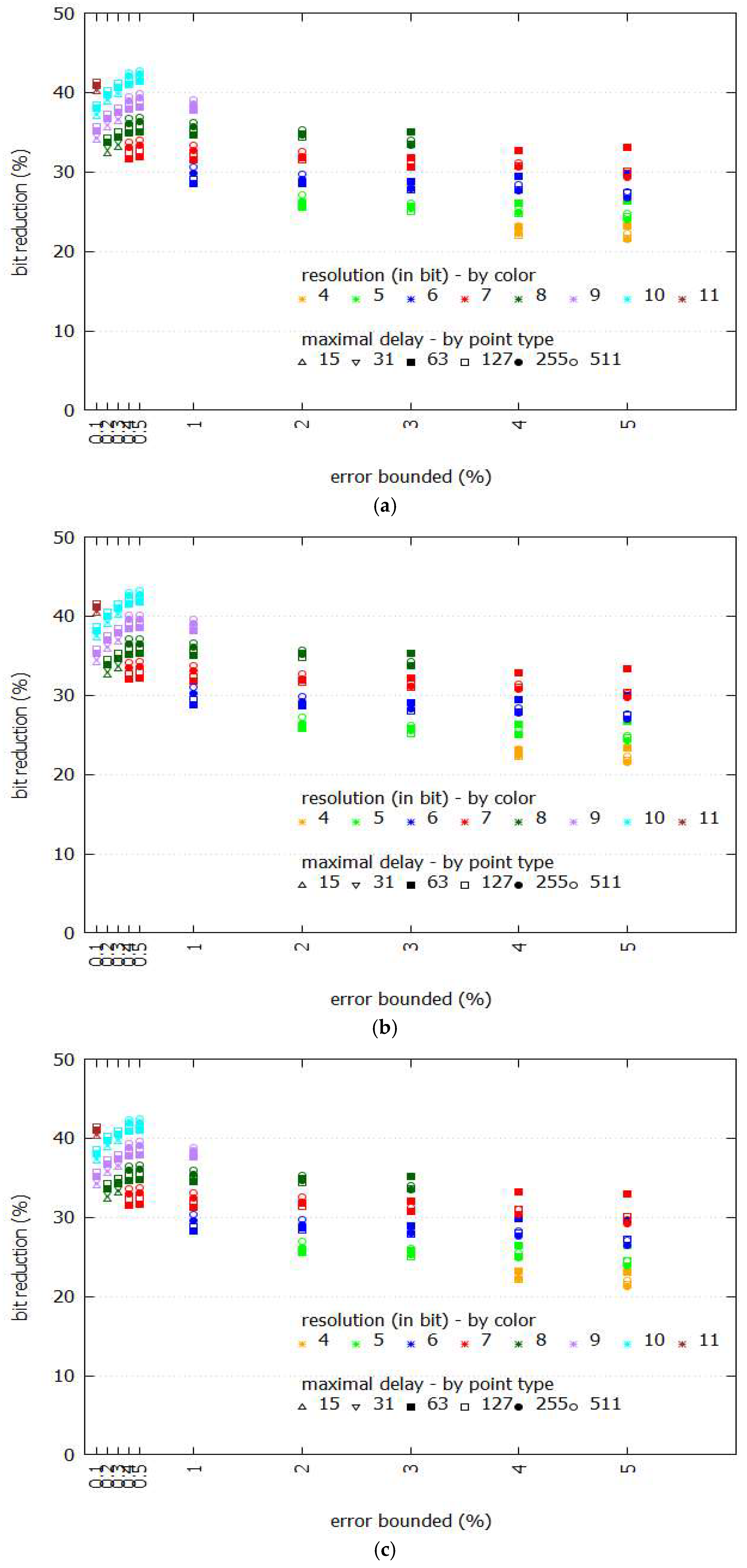
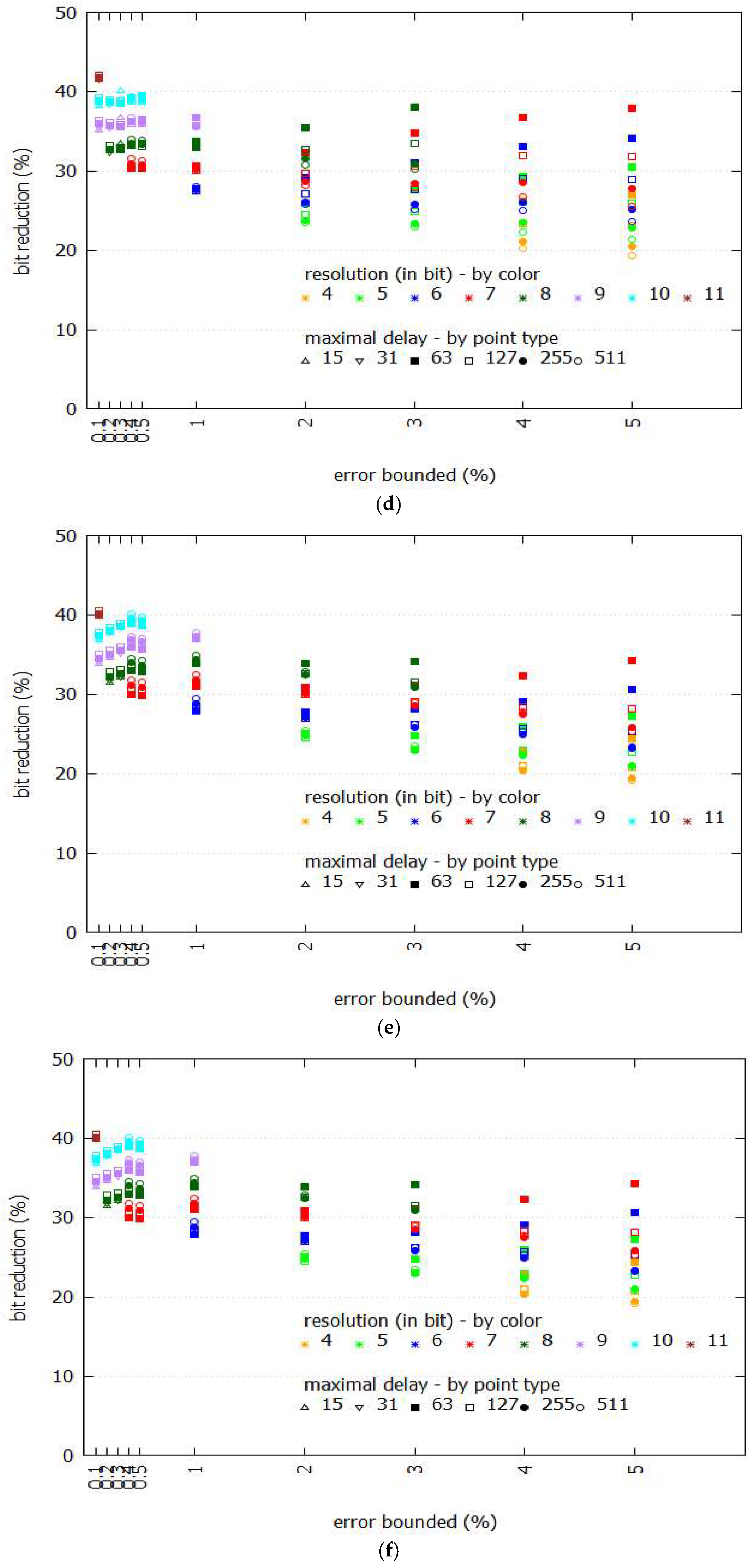
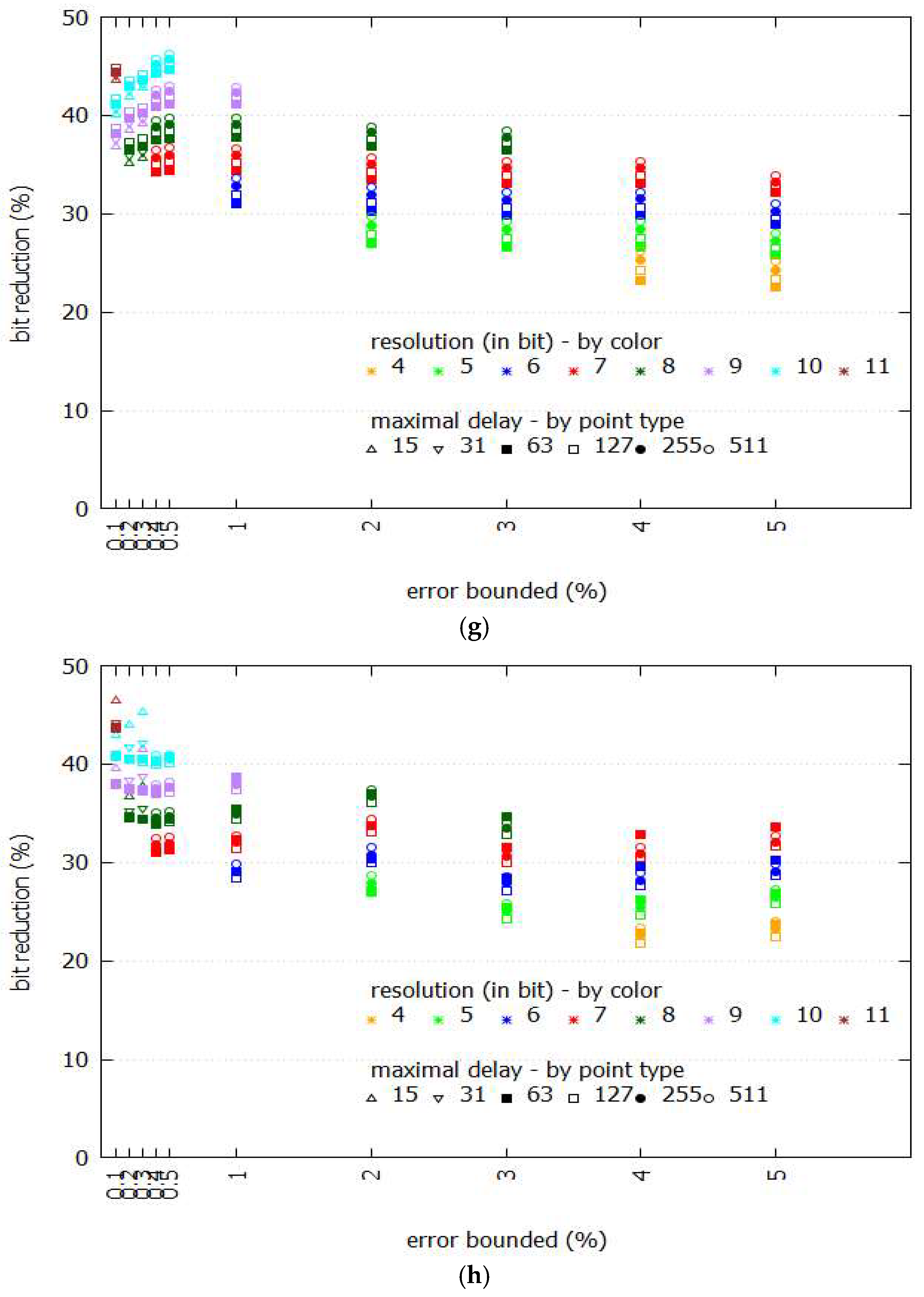
Figure 5 shows the performance comparison between Swing-RR and Swing filter given different sizes of BEPLA, where maximal delays and resolutions are discriminated by different point types and colors, respectively. Specifically, we calculate the ratio of the size (in bits) of the two BEPLAs generated by Swing-RR and Swing filter. For all eight datasets, Swing-RR uses fewer bits significantly than Swing filter does. For typical error bounds ranging from 0.5% to 5%, when comparing with the number of bits needed by Swing filter to represent its BEPLA, only 20–35% of bits are consumed by Swing-RR. Even for a much smaller error bound, e.g., 0.1–0.4%, Swing-RR needs only 30–45% of bits required by Swing filter.
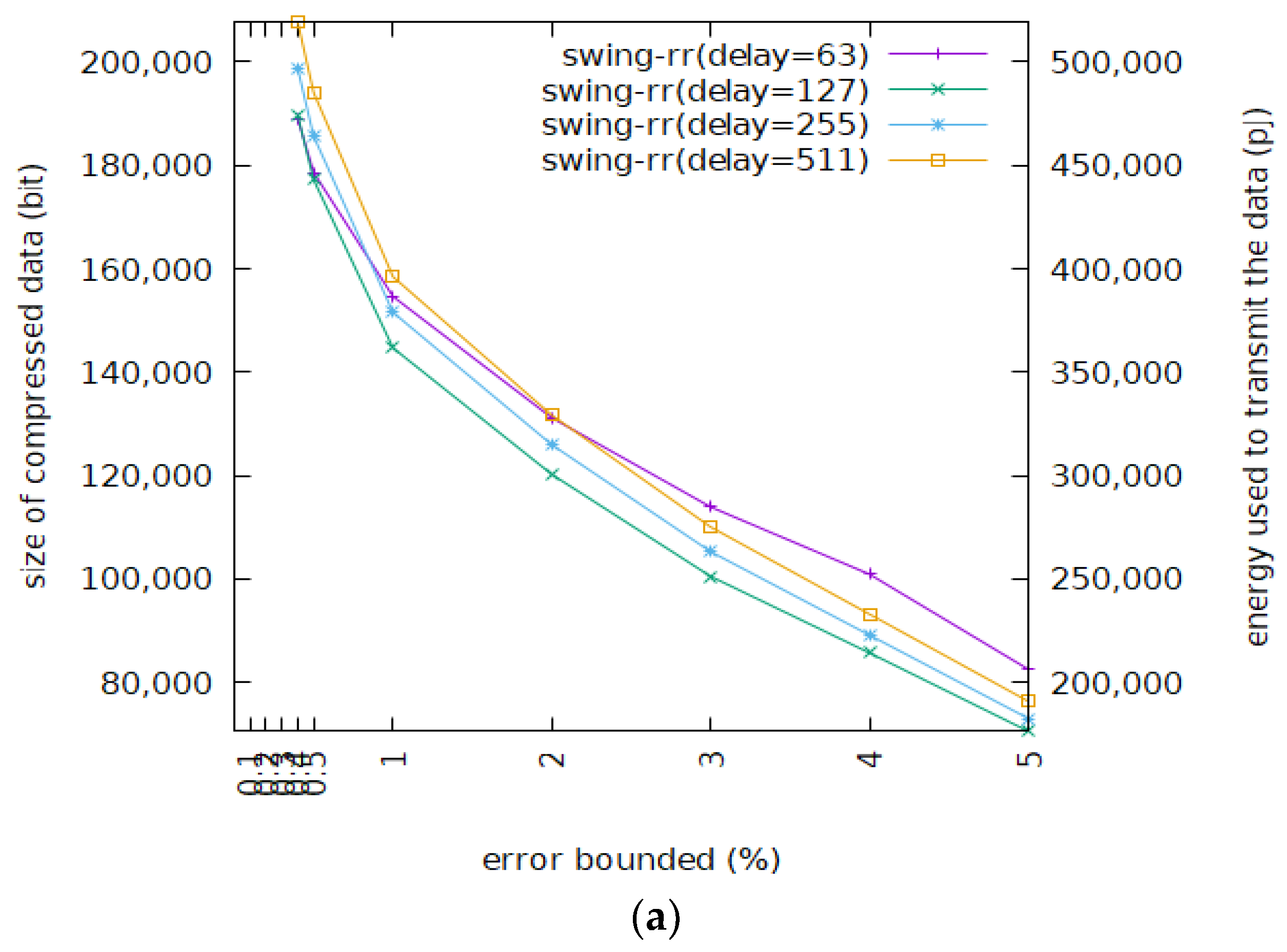
The upper bound H(t) and lower bound G(t) of ε restrict the space of BEPLA. As shown in Figure 6 and Figure 7, when the error bound is enlarged, the bits used to represent BEPLA generated by both Swing-RR and Swing filter are further reduced as expected. Since the figures for all datasets are very similar, only a part of them is shown.
For the eight datasets employed, Swing-RR using the minimal resolution (please refer to Equation (9) and Table 1) always generates the best compression ratios. As shown in Figure 5a–h, when the error bound is set to 4% or 5%, Swing-RR with minimal resolution (4 bits) has the most significant bit reduction. Compared to the number of bits needed by Swing filter to represent its BEPLA, only about 20% of bits (colored in orange) are consumed by Swing-RR. When the error bound is set to 2% or 3%, Swing-RR with minimal resolution (5 bits) has the most significant bit reduction again, only about 25% (colored in green) of bits are required, compared to that needed by Swing filter. For other error bounds, similar results are conducted.
In most scenarios, given an error bound, the locations of points are strongly related to their colors (which represent the resolution), as shown in Figure 5a–h. In fact, the differences on numbers of line segments of BEPLA generated by Swing-RR with different resolutions and maximal delays are small, compared to the total number of line segments. We will show this in the following. Also, please refer to Equations (7) and (8), because the change of k (i.e., the number of line segments) is small, p (i.e., bits for resolution), and q (i.e., bits for maximal delay) play more important roles in affecting the size of compressed data.
On the other hand, given an error bound, the resolution plays an important role in reducing size of compressed data than the maximal delay does. In Figure 5a–h, the points of different point types (which represent the maximal delay) but in a same color (which shows the resolution) are very close.
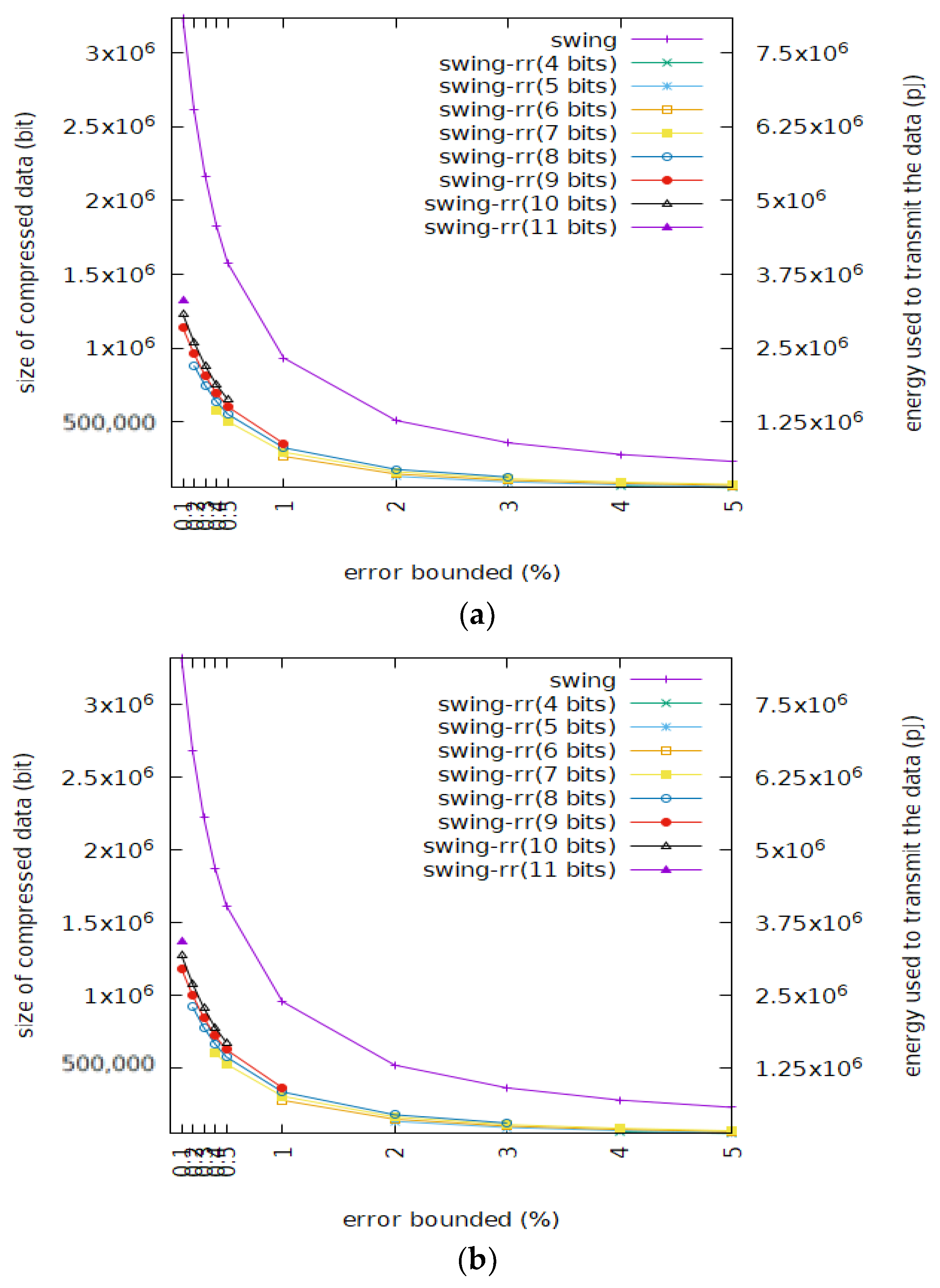
Figure 6 shows the sizes of the BEPLA generated by Swing filter and Swing-RR and their energy consumption, given different resolutions to the Cricket_X dataset. Scenarios on maximal delays of 63 and 127 are shown. Here energy consumption EC is defined as
where N is the number of bit actually transmitted, and U_E is the energy consumed for delivering a bit, a typical value of which is 2.5 PJ/bit (i.e., pico joule per bit) [39]. As described above, Swing-RR outperforms Swing filter significantly. Swing-RR with the minimal resolution achieves a much better compression than Swing filter does. Since IoT data are transmitted all year long, maybe continuously or intermittently, from a long term viewpoint, the accumulatively saved energy should be huge. Note that Figure 6a and Figure 6b are very similar.
EC = N * U_E
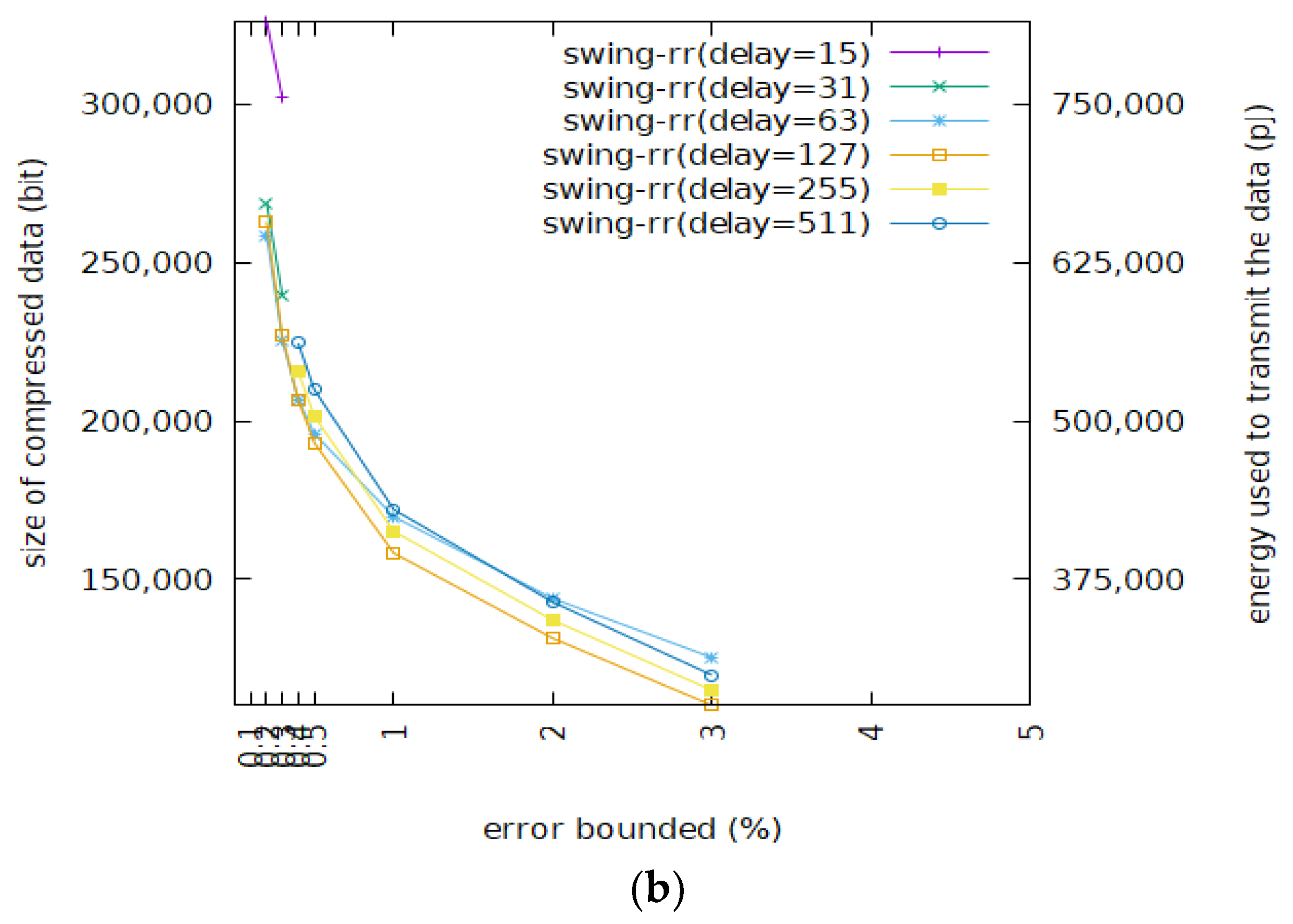
Figure 7 shows the size of the BEPLA generated by Swing filter and Swing-RR and their energy consumption, given different maximal delays to the wafer dataset. For a typical error bound, i.e., from 0.5% to 5%, and resolutions, i.e., 7 and 8 bits, Swing-RR with a maximal delay of 127 or 255 compresses the wafer dataset better than Swing-RR with a maximal delay of 63 or 511 does. When the maximal delay is too short, as mentioned before, long line segments will be cut. When the maximal delay is longer than the lengths of most line segments, some bits allocated to record the length will not be used, thus bit efficiency is reduced.
As described above, Slide filter and Cont-PLA mutually outperform each other given different datasets, while Mixed-PLA outperforms Swing-filter, Slide filter, and Cont-PLA on the eight real world datasets [29,34]. The size of BEPLA generated by Mixed-PLA is about 50–60% of that produced by Swing filter. These methods focus on how to minimize the number of line segments. Furthermore, when using minimal resolution, Swing-RR requires only 20–25% of bits. Of course, the accumulatively saved energy is also huge.
3.3. Number of Segments and Their Length
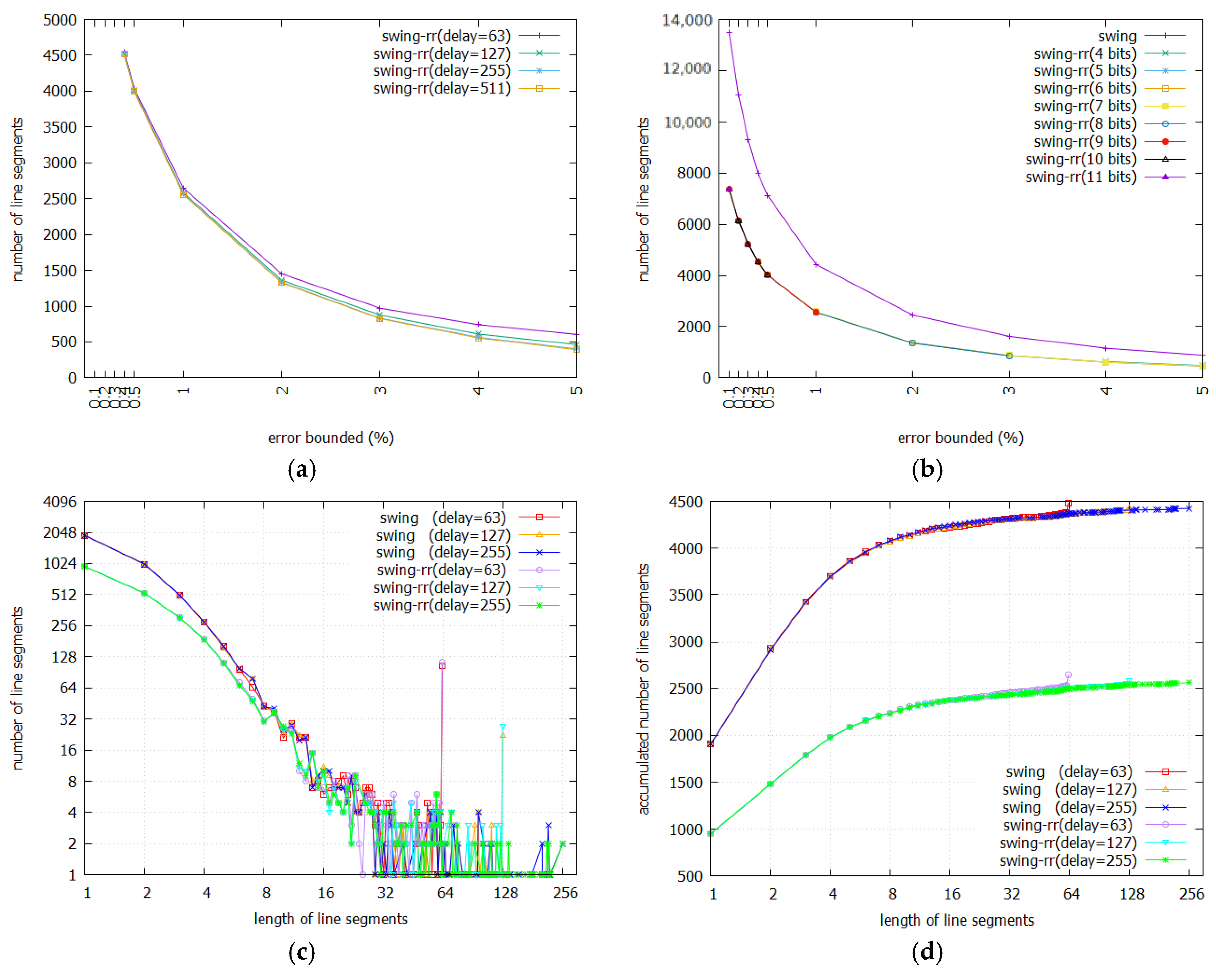
Figure 8a,b show the numbers of line segments required to represent BEPLA generated by Swing-RR on the Lighting7 dataset given different maximal delays and resolutions. For an error bound, as mentioned above, the differences of numbers of line segments generated on different maximal delays are small, compared to the total number of line segments. On the other hand, the bit reduction caused by using fewer bits to represent the length of line segments is trivial. This is also true for different resolutions.
In fact, the distribution of numbers of line segments and their lengths follows power law [40]. Most line segments are short. Only a small portion is long. As shown in Figure 8c, given the Lighting7 dataset, when error bound is 1%, the numbers of short line segments produced by Swing filter and Swing-RR on different maximal delays (63, 127, 255) are not far away. The peaks in length 63 for both schemes show that some line segments are longer than 63. So long line segments are cut at this length. As shown in Figure 8a, when the error bound is 1%, roughly 2,500 line segments in the BEPLA are generated by Swing-RR on different maximal delays. Among them, as shown in Figure 8c, there are about 1000, the length of which is 1, and about 500, the length of which is 2. More than one half of line segments are very short. In fact, less than 100 line segments are longer than 63. As a result, it might be worth to specify a smaller maximal delay and thus represent the lengths of line segments with fewer bits.
Further, the length of an IP header is about 32 bytes (between 20 and 60 bytes), meaning that 256 bits are ordinarily accompanied with the delivered data of a line segment. The energy consumed for transmitting an IP header, denoted by EIH, is defined as
where M is the number of line segments generated. As shown in Figure 8, we can see that the total numbers of line segments produced by Swing filter are higher than those yielded by Swing-RR. For example, in Figure 8b, when error bounded is 1, the numbers generated by Swing-RR are about 2500, whereas those produced by Swing filter are about 4500. The difference between the two consumed energies is 259 * 2.5 * (4500 − 2500) PJ. The phenomenon also occurs in Figure 8d, i.e., accumulated number of line segments. In Figure 8, we do not show the corresponding energy since it is trivial. Only M is shown. We can obtain the consumed energy by multiplying M with 256 * 2.5 PJ.
EIH = 256 * 2.5 PJ * M
3.4. Mean Square Error
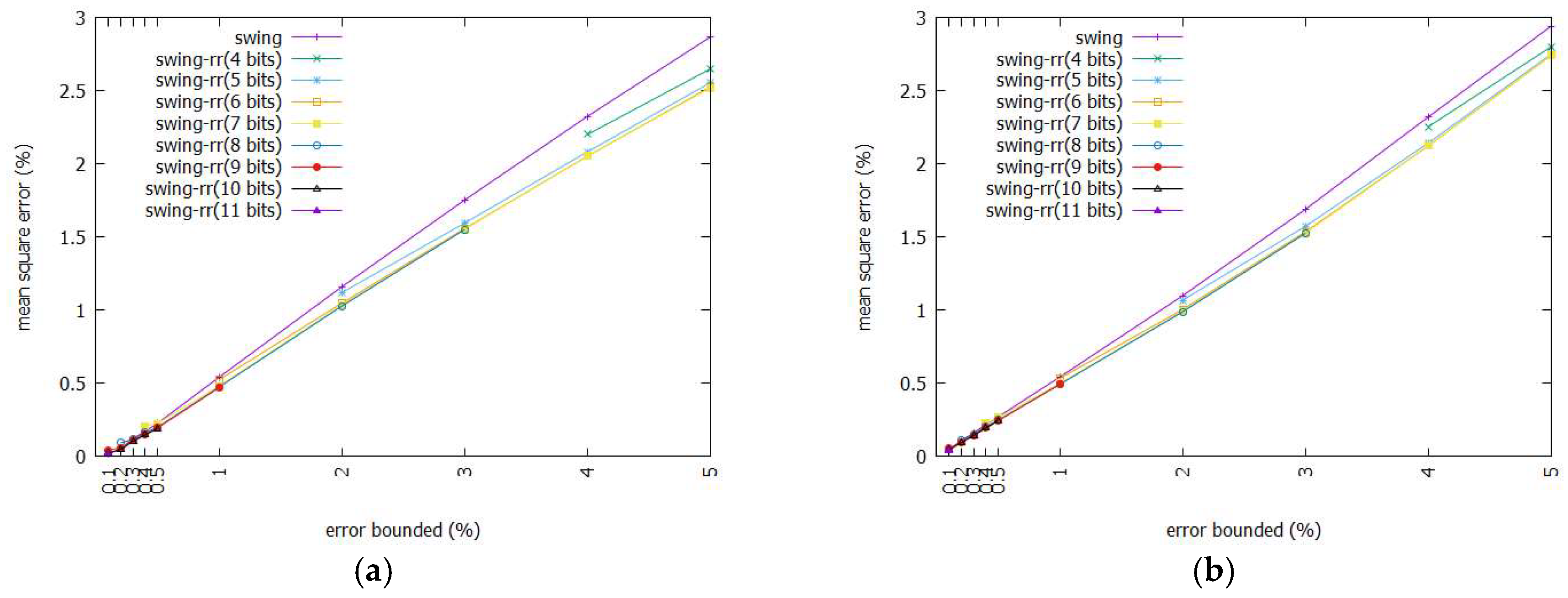
Figure 9 shows the MSE between the original data and BEPLA generated by Swing filter and Swing-RR, given the FaceFour dataset. Swing filter yields joint BEPLA, in which the start point of a line segment is the stop point of its immediate previous line segment. To extend the line segments as long as possible and thus minimize the number of line segments, the line segments generated by Swing filter usually reach the upper H(t) or lower bound G(t). On the other hand, the available approximated data points for Swing-RR are seldom close to H(t) or G(t). When Swing-RR is employed, the start point of each line segment in disjoint BEPLA is the coded data point nearest to the original data point. Furthermore, most line segments are very short. In fact, there are more than one half of line segments, the lengths of which are 1 or 2 time ticks. For these short line segments, it is expected that the stop points are also individually close to their own original data. As a result, BEPLA produced by Swing-RR has smaller MSE than that yielded by Swing filter.
When resolution increases, many more coded data points will be there between the upper and lower bounds. The MSE between the original data and BEPLA generated by Swing-RR with a smaller resolution is further reduced, as shown in Figure 9a,b.
4. Conclusions
In Industry 4.0, sensors play a very important role in manufacturing automation. However, the big data generated by these sensors consumes a lot of energy, for transmitting data from sensors to data center, and data storage in the data centers. The best practices to improve data center power saving include reduction of storage disk space, and network port power consumption. Data compression is a common approach to reduce the amount of big data transmitted via networks. BEPLA retains a certain level of quality of the original sensor data for later analysis. Previous methods focused on how to extend the line segments as long as possible, thus minimizing the number of line segments in BEPLA. However, the length of a line segment, or the length that a line segment can extend, largely depends on the given error bound and data variation.
In this paper, Swing-RR is presented to produce disjoint BEPLA with Resolution Reduction for sensor data compression. To the best of authors’ knowledge, it is the first attempt to take Resolution Reduction into consideration for BEPLA. The real-world datasets [37] are used to evaluate the performance and energy consumption of Swing-RR. Our experimental results show that Swing-RR outperforms Swing filter. For typical error bounds, i.e., 0.5–5%, Swing-RR with minimal resolution achieves much better compression ratios. Swing-RR uses 7 (for 0.5%) to 4 (for 5%) bits, rather than 32 bits, to store the approximated data point. Refer to Equations (7) and (8), since p decreases significantly, the size reduction of BEPLA is obvious. Compared to the number of bits needed by Swing filter to represent its BEPLA, Swing-RR uses only 20–25% of bits, while state-of-the-art methods utilize 50–60% of bits. As a result, fewer bits are transmitted in the network and less disk space are required to store the sensor data in the data center. Generally, the power consumption is largely reduced. As well, the MSE of BEPLA generated by Swing-RR is smaller than that produced by Swing filter.
The resolution plays a more important role than the maximal delay. In this study, for all datasets, Swing-RR using the minimal resolution always yields better compression ratios than using a higher resolution does. Most line segments are short. Only a small portion is long. Thus, it is worth using fewer bits to encode the lengths of segments.
The time and space complexities of Swing-RR are both O(1). This makes Swing-RR suitable for sensors with limited resources and energy.
In this paper, only temporal correlation in sensor data is leveraged. Data and spatial correlations [26] are currently under investigation. As well, we are going to explore more complex data structures, e.g., convex hull used in previous methods [31,34].
Also, we assume that the collected data are precise. In reality, there can be some bias in data collection. For example, the environments monitored by sensors are under attack [41], and the sensed data are contaminated. Depending on the roles, edge nodes can preprocess the data before the data are sent to their data centers. They can do nothing and send the raw data. Or, they can remove the outliers, predict the missing data, and measure the robustness of the network. The authors will further study these issues in the future.
Author Contributions
J.-W.L. provides ideas, writes the paper and performs those experiments. S.-w.L. verifies the experimental results and suggests how to tune the parameters of these experiments. F.-Y.L. reorganizes paper structure, polishes English description and performs energy-consumption experiments.
Funding
This research was supported in part by National Science Council, Taiwan, under grant MOST 107-2221-E-029-011-.
Conflicts of Interest
The authors declare no conflict of interest.
References
- Wu, S.; Zuo, M.J. Linear and nonlinear preventive maintenance models. IEEE Trans. Reliab. 2010, 59, 242–249. [Google Scholar] [CrossRef]
- Shang, Y. Vulnerability of networks: Fractional percolation on random graphs. Phys. Rev. E 2014, 89, 012813. [Google Scholar] [CrossRef] [PubMed]
- Shehabi, A.; Smith, S.; Sartor, D.; Brown, R.; Herrlin, M.; Koomey, J.; Masanet, E.; Horner, N.; Azevedo, I.; Lintner, W. United States Data Center Energy Usage Report; LBNL-1005775; Lawrence Berkeley National Laboratory: Berkeley, CA, USA, 2016. [Google Scholar]
- Baliga, J.; Ayre, R.W.A.; Hinton, K.; Tucker, R.S. Green cloud computing: Balancing energy in processing, storage, and transport. Proc. IEEE 2011, 99, 149–167. [Google Scholar] [CrossRef]
- Huang, X.; Hu, T.; Ye, C.; Xu, G.; Wang, X.; Chen, L. Electric load data compression and classification based on deep stacked auto-encoders. Energies 2019, 12, 653. [Google Scholar] [CrossRef]
- Kawahara, M.; Chiu, Y.J.; Berger, T. High-speed software implementation of Huffman coding. In Proceedings of the 98th Data Compression Conference, Snowbird, UT, USA, 30 March–1 April 1998; p. 553. [Google Scholar]
- Marcelloni, F.; Vecchio, M. A simple algorithm for data compression in wireless sensor networks. IEEE Commun. Lett. 2008, 12, 411–413. [Google Scholar] [CrossRef]
- Javed, M.Y.; Nadeem, A. Data compression through adaptive Huffman coding schemes. In Proceedings of the IEEE TENCON 2000, Kuala Lumpur, Malaysia, 24–27 September 2000; pp. 187–190. [Google Scholar]
- Tharini, C.; Ranjan, P.V. Design of modified adaptive Huffman data compression algorithm for wireless sensor network. J. Comput. Sci. 2009, 5, 466–470. [Google Scholar] [CrossRef]
- Lin, C.C.; Chuang, C.C.; Chiang, C.W.; Chang, R.I. A novel data compression method using improved JPEG-LS in wireless sensor networks. In Proceedings of the 12th International Conference on Advanced Communication Technology, Phoenix Park, Korea, 7–10 February 2010; pp. 346–351. [Google Scholar]
- Higgins, G.; Mc Ginley, B.; Glavin, M.; Jones, E. Low power compression of EEG signals using JPEG2000. In Proceedings of the 4th International Conference on Pervasive Computing Technologies for Healthcare, Munich, Germany, 22–25 March 2010. [Google Scholar]
- Bendifallah, A.; Benzid, R.; Boulemden, M. Improved ECG compression method using discrete cosine transform. Electron. Lett. 2011, 47, 1–2. [Google Scholar] [CrossRef]
- Chen, J.; Ma, J.; Zhang, Y.; Shi, X. A wavelet-based ECG compression algorithm using Golomb codes. In Proceedings of the 2006 IEEE International Conference on Communications, Circuits, and Systems, Guilin, China, 25–28 June 2006; pp. 130–133. [Google Scholar]
- Fang, J.; Li, H. Hyperplane-based vector quantization for distributed estimation in wireless sensor networks. IEEE Trans. Inf. Theory 2009, 55, 5682–5699. [Google Scholar] [CrossRef]
- Wang, Y.C.; Hsieh, Y.Y.; Tseng, Y.C. Multiresolution spatial and temporal coding in a wireless sensor network for long-term monitoring applications. IEEE Trans. Comput. 2009, 58, 827–838. [Google Scholar] [CrossRef]
- Makarenko, A.; Whyte, H.D. Decentralized data fusion and control in active sensor networks. In Proceedings of the 7th International Conference on Information Fusion, Stockholm, Sweden, 28 June–1 July 2004; pp. 479–486. [Google Scholar]
- Yuan, W.; Krishnamurthy, S.V.; Tripathi, S.K. Synchronization of multiple levels of data fusion in wireless sensor networks. In Proceedings of the IEEE Global Telecommunications Conference, Riverside, CA, USA, 1 December 2003; pp. 221–225. [Google Scholar]
- Sharaf, M.A.; Beaver, J.; Labrinidis, A.; Chrysanthis, P.K. TiNA: A scheme for temporal coherency-aware in-network aggregation. In Proceedings of the 3rd ACM International Workshop on Data Engineering for Wireless and Mobile Access, Pittsburgh, PA, USA, 19 September 2003; pp. 69–76. [Google Scholar]
- Yoon, S.; Shahabi, C. The clustered aggregation (CAG) technique leveraging spatial and temporal correlations in wireless sensor networks. ACM Trans. Sens. Netw. 2007, 3, 3. [Google Scholar] [CrossRef]
- Goel, S.; Imielinski, T. Prediction-based monitoring in sensor network: Taking lessons from MPEG. Comput. Commun. Rev. 2001, 31, 82–98. [Google Scholar] [CrossRef]
- Choi, K.; Kim, M.H.; Chae, K.J.; Park, J.J.; Joo, S.S. An efficient data fusion and assurance mechanism using temporal and spatial correlations for home automation networks. IEEE Trans. Consum. Electron. 2009, 55, 1330–1336. [Google Scholar] [CrossRef]
- Luo, H.; Luo, J.; Liu, Y.; Das, S.K. Adaptive data fusion for energy efficient routing in wireless sensor networks. IEEE Trans. Comput. 2006, 55, 1286–1299. [Google Scholar]
- Kumar, R.; Wolenetz, M.; Agarwalla, B.; Shin, J.; Hutto, P.; Paul, A.; Ramachandran, U. DFuse: A framework for distributed data fusion. In Proceedings of the 1st ACM International Conference on Embedded Networked Sensor Systems, Los Angeles, CA, USA, 5 November 2003; pp. 114–125. [Google Scholar]
- Jin, G.Y.; Park, M.S. CAC: Context adaptive clustering for efficient data aggregation in wireless sensor networks. Lect. Notes Comput. Sci. 2006, 3976, 1132–1137. [Google Scholar]
- Lee, S.; Yoo, J.; Chung, T. Distance-based energy efficient clustering for wireless sensor networks. In Proceedings of the 29th Annual IEEE International Conference on Local Computer Networks, Tampa, FL, USA, 16–18 November 2004; pp. 567–568. [Google Scholar]
- Chang, R.I.; Li, M.H.; Chuang, P.; Lin, J.W. Bounded error data compression and aggregation in wireless sensor networks. In Smart Sensors Networks, Communication Technologies and Intelligent Applications; A Volume in Intelligent Data-Centric Systems; Xhafa, F., Leu, F.Y., Hung, L.L., Eds.; Elsevier: London, UK, 2017; pp. 143–157. [Google Scholar]
- Hakimi, S.L.; Schmeichel, E.F. Fitting polygonal functions to a set of points in the plane. CVGIP Graph. Models Image Proc. 1991, 53, 132–136. [Google Scholar] [CrossRef]
- Imai, H.; Iri, M. An optimal algorithm for approximating a piecewise linear function. J. Inf. Proc. 1986, 9, 159–162. [Google Scholar]
- Xie, Q.; Pang, C.; Zhou, X.; Zhang, X.; Deng, K. Maximum error-bounded piecewise linear representation for online stream approximation. VLDB J. 2014, 23, 915–937. [Google Scholar] [CrossRef]
- Zhao, H.; Dong, Z.; Li, T.; Wang, X.; Pang, C. Segmenting time series with connected lines under maximum error bound. Inf. Sci. 2016, 345, 1–8. [Google Scholar] [CrossRef]
- Elmeleegy, H.; Elmagarmid, A.K.; Cecchet, E.; Aref, W.G.; Zwaenepoel, W. Online piece-wise linear approximation of numerical streams with precision guarantees. Proc. VLDB Endow. 2009, 2, 145–156. [Google Scholar] [CrossRef]
- O’Rourke, J. An on-line algorithm for fitting straight lines between data ranges. Commun. ACM 1981, 24, 574–578. [Google Scholar] [CrossRef]
- Gritzali, F.; Papakonstantinou, G. A fast piecewise linear approximation algorithm. Signal Proc. 1983, 5, 221–227. [Google Scholar] [CrossRef]
- Luo, G.; Yi, K.; Cheng, S.W.; Li, Z.; Fan, W.; He, C.; Mu, Y. Piecewise linear approximation of streaming time series data with max-error guarantees. In Proceedings of the 2015 IEEE 31st International Conference on Data Engineering, Seoul, Korea, 13–17 April 2015; pp. 173–184. [Google Scholar]
- Malash, G.F.; El-Khaiary, M.I. Piecewise linear regression: A statistical method for the analysis of experimental adsorption data by the intraparticle-diffusion models. Chem. Eng. J. 2010, 163, 256–263. [Google Scholar] [CrossRef]
- Shang, Y. Resilient multiscale coordination control against adversarial nodes. Energies 2018, 11, 1844. [Google Scholar] [CrossRef]
- Chen, Y.; Keogh, E.; Hu, B.; Begum, N.; Bagnall, A.; Mueen, A.; Batista, G. The UCR Time Series Classification Archive 2015. Available online: http://www.cs.ucr.edu/~eamonn/time_series_data/ (accessed on 7 July 2018).
- IEEE Computer Society. IEEE Standard for Floating-Point Arithmetic. Available online: IEEE Standard 754-2008. https://ieeexplore.ieee.org/document/4610935 (accessed on 7 July 2018).
- Walke, W.W.; Hidaka, Y. Next-Generation Interconnect Research at Fujitsu Laboratories. Fujitsu Sci. Technol. J. 2012, 48, 218–222. [Google Scholar]
- Clauset, A.; Shalizi, C.R.; Newman, M.E.J. Power-law distributions in empirical data. SIAM Rev. 2009, 51, 661–703. [Google Scholar] [CrossRef]
- Shang, Y. Subgraph robustness of complex networks under attacks. IEEE Trans. Syst. Man Cybern. Syst. 2019, 49, 821–832. [Google Scholar] [CrossRef]
Figure 1.
Given a bounded error ε for a time series y(t), upper bound H(t) = y(t) + ε, and lower bound G(t) = y(t) − ε, are defined.
Figure 1.
Given a bounded error ε for a time series y(t), upper bound H(t) = y(t) + ε, and lower bound G(t) = y(t) − ε, are defined.

Figure 2.
BEPLA. In (a), joint BEPLA, two joint line segments that share an endpoint are used to approximate to y(t) shown in Figure 1. In (b), disjoint BEPLA, two disjoint line segments that do not share endpoints are used to approximate to y(t). In fact, between them, there is a hidden line segment (dashed), the length of which is one time tick.

Figure 3.
BEPLA with resolution reduction. (a) Joint BEPLA. (b) Disjoint BEPLA. Coded data points are depicted as black circles.
Figure 3.
BEPLA with resolution reduction. (a) Joint BEPLA. (b) Disjoint BEPLA. Coded data points are depicted as black circles.

Figure 4.
Swing-RR. (a) Process first and second data points. (b) Process third data point. (c) Process fourth data point. (d) Process fifth data point. (e) Generate a line segment. (f) Increase the resolution.
Figure 4.
Swing-RR. (a) Process first and second data points. (b) Process third data point. (c) Process fourth data point. (d) Process fifth data point. (e) Generate a line segment. (f) Increase the resolution.

Figure 5.
Performance comparison between Swing-RR and Swing filter in the size of BEPLA. (a) Cricket_X; (b) Cricket_Y; (c) Cricket_Z; (d) FaceFour; (e) Lignting2; (f) Lighting7; (g) MoteStrain; (h) wafer.
Figure 5.
Performance comparison between Swing-RR and Swing filter in the size of BEPLA. (a) Cricket_X; (b) Cricket_Y; (c) Cricket_Z; (d) FaceFour; (e) Lignting2; (f) Lighting7; (g) MoteStrain; (h) wafer.


Figure 6.
Size of compressed data and data delivery energy consumption of Swing filter and Swing-RR where the latter is shown given different resolutions. (a) Cricket_X (delay = 63); (b) Cricket_ X (delay = 127)
Figure 6.
Size of compressed data and data delivery energy consumption of Swing filter and Swing-RR where the latter is shown given different resolutions. (a) Cricket_X (delay = 63); (b) Cricket_ X (delay = 127)

Figure 7.
Size of compressed data and data delivery energy consumption of Swing-RR on different maximal delays given Wafer. (a) Wafer (resolution = 7 bits); (b) Wafer (resolution = 8 bits).
Figure 7.
Size of compressed data and data delivery energy consumption of Swing-RR on different maximal delays given Wafer. (a) Wafer (resolution = 7 bits); (b) Wafer (resolution = 8 bits).


Figure 8.
Number of line segments and their distribution according to segment length. (a) Lighting7 (resolution = 7 bits). (b) Lighting7 (delay = 127). (c) Lighting7 (ε = 1%, resolution = 7 bits). (d) Lighting7 (ε = 1%, resolution = 7 bits).
Figure 8.
Number of line segments and their distribution according to segment length. (a) Lighting7 (resolution = 7 bits). (b) Lighting7 (delay = 127). (c) Lighting7 (ε = 1%, resolution = 7 bits). (d) Lighting7 (ε = 1%, resolution = 7 bits).

Figure 9.
MSE of BEPLA generated by Swing-RR and Swing filter. (a) FaceFour (delay = 127). (b) MoteStrain (delay = 127).
Figure 9.
MSE of BEPLA generated by Swing-RR and Swing filter. (a) FaceFour (delay = 127). (b) MoteStrain (delay = 127).


Table 1.
Minimal resolution (in bits) for error bounds.
| Error Bound (%) | 0.1 | 0.2 | 0.3 | 0.4 | 0.5 | 1 | 2 | 3 | 4 | 5 |
| Minimal Resolution (Bits) | 9 | 8 | 8 | 7 | 7 | 6 | 5 | 5 | 4 | 4 |
Table 2.
Dataset description 1.
| Dataset | Length | Minimal | Maximal |
|---|---|---|---|
| Cricket_X | 117,000 | −4.766200 | 11.494000 |
| Cricket_Y | 117,000 | −9.774500 | 6.838500 |
| Cricket_Z | 117,000 | −4.758300 | 11.924000 |
| FaceFour | 30,800 | −4.687600 | 5.908100 |
| Lignting2 | 38,220 | −1.396000 | 23.131000 |
| Lignting7 | 22,330 | −1.781200 | 17.413000 |
| MoteStrain | 105,168 | −8.409300 | 2.468400 |
| wafer | 152,000 | −3.054000 | 11.787000 |
1 The precision of data points is six digits after the decimal point.
Table 3.
Scenario examined in the experiment.
| Error Bound (ε) | Resolution | Maximal Delay |
|---|---|---|
| 0.1% | 9, 10, 11 | 15, 31, 63, 127 |
| 0.2% | 8, 9, 10 | 15, 31, 63, 127 |
| 0.3% | 8, 9, 10 | 15, 31, 63, 127 |
| 0.4% | 7, 8, 9, 10 | 63, 127, 255, 511 |
| 0.5% | 7, 8, 9, 10 | 63, 127, 255, 511 |
| 1% | 6, 7, 8, 9 | 63, 127, 255, 511 |
| 2% | 5, 6, 7, 8 | 63, 127, 255, 511 |
| 3% | 5, 6, 7, 8 | 63, 127, 255, 511 |
| 4% | 4, 5, 6, 7 | 63, 127, 255, 511 |
| 5% | 4, 5, 6, 7 | 63, 127, 255, 511 |
© 2019 by the authors. Licensee MDPI, Basel, Switzerland. This article is an open access article distributed under the terms and conditions of the Creative Commons Attribution (CC BY) license (http://creativecommons.org/licenses/by/4.0/).
Share and Cite
MDPI and ACS Style
Lin, J.-W.; Liao, S.-w.; Leu, F.-Y. Sensor Data Compression Using Bounded Error Piecewise Linear Approximation with Resolution Reduction. Energies 2019, 12, 2523. https://doi.org/10.3390/en12132523
AMA Style
Lin J-W, Liao S-w, Leu F-Y. Sensor Data Compression Using Bounded Error Piecewise Linear Approximation with Resolution Reduction. Energies. 2019; 12(13):2523. https://doi.org/10.3390/en12132523
Chicago/Turabian StyleLin, Jeng-Wei, Shih-wei Liao, and Fang-Yie Leu. 2019. "Sensor Data Compression Using Bounded Error Piecewise Linear Approximation with Resolution Reduction" Energies 12, no. 13: 2523. https://doi.org/10.3390/en12132523
Note that from the first issue of 2016, this journal uses article numbers instead of page numbers. See further details here.