On the Use of Causality Inference in Designing Tariffs to Implement More Effective Behavioral Demand Response Programs

Abstract

Providing a price tariff that matches the randomized behavior of residential consumers is one of the major barriers to demand response (DR) implementation. The current trend of DR products provided by aggregators or retailers are not consumer-specific, which poses additional barriers for the engagement of consumers in these programs. In order to address this issue, this paper describes a methodology based on causality inference between DR tariffs and observed residential electricity consumption to estimate consumers’ consumption elasticity. It determines the flexibility of each client under the considered DR program and identifies whether the tariffs offered by the DR program affect the consumers’ usual consumption or not. The aim of this approach is to aid aggregators and retailers to better tune DR offers to consumer needs and so to enlarge the response rate to their DR programs. We identify a set of critical clients who actively participate in DR events along with the most responsive and least responsive clients for the considered DR program. We find that the percentage of DR consumers who actively participate seem to be much less than expected by retailers, indicating that not all consumers’ elasticity is effectively utilized.

1. Introduction

1.1. Context and Motivation

Demand response (DR) incentivizes changes in customer energy usage patterns to reward lower electricity use at times when system reliability is jeopardized, the price of electricity is higher, or the grid has difficulties in delivering the electricity to the consumers. Electric utilities essentially consider DR as an effective way to reduce customer demand for electricity delivered over the grid. This change in the consumption behavior of the consumer can be brought about by two methods. The first method (active participation) relies on the consumer to alter how they use their appliances that they already own by stimulation through different pricing mechanisms, customer engagement platforms, and alerts of grid stability via text or mobile applications. The other method (passive participation) requires the consumers to purchase or install additional devices that use less electricity. The main issues with the active participation of residential consumers in DR programs are that gains may be lost as soon as the program ends, may inadvertently lead to increased electricity use, and active periods of participation may not coincide with required DR periods.

The retailers (or aggregators) encourage the consumers to participate in various DR strategies that are influenced by time-of-use (TOU) pricing, which is a static pricing mechanism, and direct load control (DLC) strategy, real-time pricing (RTP), and critical-peak pricing (CPP), which are dynamic pricing mechanisms [1]. Residential electricity consumers are usually unwilling to participate in volatile pool markets. The use of a short-term DR program with time-varying prices in residential DR will have little to no electricity consumption elasticity from consumers [2]. There is no guarantee of a response from a consumer as it directly depends on its willingness to reduce consumption (unless the consumer is in a direct load control program). The TOU strategy supports DR by inducing demand shifts from high price periods to lower pricing periods as it provides at least two pricing levels—one high price during peak hours (afternoons) and the other hours having a lower off-peak pricing. The drawback is that the TOU pricing works on a predicted average marginal cost for the peak hours and there are not enough incentives for the consumers when they provide DR services during critical grid issue periods. The assumption that serving peak demand is more expensive than serving off-peak is not true anymore as there could be days when consumers pay high prices for peak periods under no active capacity constraints (as these rates were fixed based on historical patterns). There may be vulnerable consumers who are not part of the peak demand problem but still end up paying for rewards for consumers who shifted their usual high peak consumption. DR programs with direct load control (DLC) take a variety of forms, including one-time signing payment, free hardware installation, and a recurring annual payment [3]. The DLC strategy corresponds to voluntary programs, which provide the utility (or aggregator) with the capability and permission from the consumer to perform direct load control on certain equipment within the household (like air conditioners, refrigerators, etc.). Nevertheless, there are times when the system peak may occur outside of the window of hours that are available for DLC from the contracted clients. This means that it is also important to consider situations when DLC is unavailable. The change in price must be large enough for customers to deem a response worthwhile, a proper communication channel for conveying the price change, and customers must have the means to shed or shift load (for example, via home-automated controls). To overcome some of these issues, it is possible to adopt a dynamic pricing mechanism that changes retail electricity prices (usually done by regulators) due to some specific conditions in the electricity systems (for example, due to expected critical peak hour). The retailers are expected to inform the consumers well before these events occur for them to be aware of this price change and take action accordingly. This would create the opportunity to aggregate a set of consumers to a block of price incentivized DR period.

The RTP provides hourly tariffs based on the price signals received by the utility from the market operator (marginal costs) on an hourly basis. However, this involves the residential consumers making hourly decisions in deciding their consumption levels if they are willing to participate in certain hours/days. This is undesirable and not practical for such disaggregated and small electricity consumers as they will not be able to get the maximum benefits from this strategy. The CPP is a variation of the TOU strategy that provides a very high price for the critical stress peak periods in the system. These prices are discretionary and are predetermined rates, which are applied during the forecasted system critical period [4,5,6].

The current residential DR programs’ engagement is far from its achievable potential because of a lack of addressing the barriers that largely vary between contracted individual consumers [7]. The aggregator and retailer must incorporate possible directions to alter consumption patterns along with their DR signals to clients, who are allowed to take free actions towards the signals they receive. This will lead to confident participation of the consumers without their current concerns of energy security and privacy. This approach, on the other hand, will cause some concerns for the retailers in the scope of reliability and security of the bids they make in the wholesale market. The accuracy of their bid highly depends on the prediction of the consumer’s behavior towards their DR signals and during the non-DR periods. Presently, retailers that send out these signals to their consumers do not know their actual response. They make basic assumptions/predictions by admitting that their consumers will reduce their demand based on price incentives (price variations between the DR and non-DR periods). In all implicit DR programs, the change in demand is considered a result of price signals seen by the consumers. This reduction is relative to the hypothetical demand that would have been observed, in the absence of the DR signal. However, in the real scenario, retailers do not know the flexibility of their contracted residential clients. If they do not make an informed bid, then a bidding high capacity would result in a penalty due to a failure in reaching the contract obligation or bidding less might result in suboptimal revenue. Furthermore, DR products can introduce more uncertainty and variability in the load forecasting task that is used to construct buying bids from retailers in the electricity market. This will require the development of new load forecasting techniques that produce a joint modelling of load and dynamic prices, where information about consumer elasticity is useful for improving the forecasting accuracy. On the other hand, demand side flexibility can also be used to reduce market imbalances due to forecast errors (e.g., from renewable energy).

The Federal Energy Regulatory Commission (FERC) estimated that the current residential DR programs in the US only engaged 10% of homes and is far from the achievable potential [8]. The DR pilot carried out by Puget Sound Energy (PSE) involving 400,000 small commercial and residential customers in 2001 to 2002 had very modest price differentials between the peak and off-peak periods [9]. On the first year, customer satisfaction was high. However, in the second phase, when the program included a monthly fee (for managing collected data), consumers saw little to no savings and many opted out of the program. This is probably because, in a recent DR status report done by Joint Research Centre (JRC) Science with the European Commission [10], it was reported that most of the business cases developed for DR do not prove to be positive for all actors involved in the DR value chain. They suggested (re)designing the new market with the capability of adopting new actors, like prosumers, EV, and other storage systems, that could typically dominate residential sectors. Designing DR programs with these capabilities could prove to be an additive incentive for consumers not to opt-out of the program. A general deduction is that the influencing factors on consumer behavior and consumption are more dynamic, which makes them less predictable so that building a common and fixed plan becomes virtually impossible [11]. Currently, retailers do not know the exact flexibility of their clients and do not know whether their residential clients react to several DR actions or products [12].

1.2. Related Work and Contributions

It is important to understand how demand changes in response to incentives or tariff. Many models integrate survey data with a detailed residential load model to identify customer elasticity for incentives. Asadinejad et al. [13] identified incentive-based elasticity at the individual appliance level (by load disaggregation) and showed that lighting had the highest elasticity, but HVAC has the highest share in the aggregated load, resulting in more effective load shifting. Klaassen et al. [14] analyzed household flexibility based on the load shifting of smart appliances and the overall peak load towards dynamic tariffs. They followed the experimental procedure of using two groups with different peak pricings and price responsiveness was assessed by comparing peak load shifts between these groups. Studies on empirical estimations of long and short-term electricity consumption elasticity using error correction, loglinear, and translog techniques showed that the elasticity is near unity, such as Baker et al. in the United Kingdom [15] and Kamerschen et al. in the United States [16]. It is not possible to predict an individual’s baseline demand with high accuracy. Some studies, such as [17,18], have used machine learning techniques, like ordinary least square regression, support vector regression, and decision tree regression, and have compared their results’ accuracy. The DSO uses these baseline consumption levels to check whether the aggregator and retailer satisfied their offers and charged them, respectively. One specific case in California with the Southern California Edison (SCE) utility has shown why the current status of DR programs still does not achieve their potential. For a period in June 2016, the California ISO charged the SCE for overages even though they saw a significant reduction in demand. This was because their 10-in-10 approach uses the 10 most recent non-event business days and it provided them a baseline prediction that was much less than the actual reduction seen. Apart from this, another issue that the utilities could face is the intentional increase in baseline consumption by consumers if they realize that a DR event could be in the near future (for example, sunny days) [19].

The EcoGrid EU experiment [20,21] disaggregated the residential consumers’ load into its constituent parts to understand the controllable resources and integrate residential DR into a balancing market. To determine consumption changes, they used a classical time-series differencing linear model to avoid collinearity problems. They found that consumers were not always price sensitive. A data-driven targeting of consumers for demand response was performed by [22,23]. They considered this approach because the DR programs are typically designed to extract a targeted level (based on the bid made by the aggregator/retailer in the market) of power from participants. Both these studies suggested that the most important statistics for a utility to manage its DR program is to typically identify the trade-off curve between DR availability and DR reliability. Throughout the literature, there is a growing consensus that a change in price (and external variables, like temperature) causes changes in electricity consumption. The correlation between these variables and electricity consumption does not imply causation. For example, electricity consumption along a day varies relative to the time of the day. Here, the time components are highly correlated to the consumption, but this does not mean they causes consumption changes.

The elasticity of consumers’ consumption behavior varies from individual to individual and utilities will benefit from knowing the elasticity their different tariff schemes create. Grouping consumers based on predicted base load profiles and determining their price elasticity to demand (such as in [24]) undermines the effective flexibility each consumer can offer. In addition, stamping a price elasticity of demand value for a consumer based on their overall consumption (such as [15,16]) further narrows down on the demand flexibility it can offer during different periods of the day. The downside of using linear models and using baseline-estimating techniques is that it removes useful information and the considered parameters will no longer relate to the absolute effects that one sees in electricity consumption changes.

Since price-based DR programs use the flexibility in price as an incentive to induce consumers to respond, one needs to define the relationship between the client’s electricity consumption and price. It has also been identified that selecting customers with high energy saving potential during a DR event day requires an accurate model. This is very difficult because no model can provide close to accurate predictions without errors that can be simulated, for example, the unexpected behavior of a consumer during particular seasons. Our approach tackles this problem by using causality inference techniques. Many confounders (variables that influences both the dependent and independent variable) affect the final consumption change made by the consumer on the day. An action or intervention, in theory, will have an effect and the causes of these effects can be studied to understand how the intervention resulted in the effect. Causes have effects, which causes other effects and the chain goes on. The magnitude of the effect depends on how the intervention affects the process.

The main original contribution from this paper is a methodology that uses causal inference theory to estimate the elasticity of domestic electricity consumption in response to dynamic tariffs. The challenge associated to the application of causal effect models is to use available information of electricity consumption from before and after a DR event instead of two different (experimental and control) groups, like in [9]. This eliminates the need for selecting, monitoring, and controlling a set of consumers (i.e., baseline group) who behave similar to clients considered for DR. A similar objective (i.e., baseline-free approach) is followed in [20], but by using a correlation-based distance between the individual loads and the real-time price and without including exogenous information, such as the ambient temperature. In contrast, the methodology proposed in this paper uses a causality-based metric and includes the effect of exogenous variables.

Our novel method identifies an individual’s consumption elasticity to DR pricing rather than grouping consumers as in [24], as such aggregated groups often lose much flexibility information at the individual level. This enables the retailer to understand the effect of a price change on consumption for every contracted DR client and identify whether a particular consumer is susceptible to DR pricing. In fact, the results negate the notion of believing that an increasing price reduces consumption, as stated in most of the literature. The proposed method also allows an understanding of whether the consumer is susceptible to either higher tariffs or lower tariffs or both, along with the hours and periods for which this is evident. Moreover, the proposed method can be used to rank clients according to their elasticity for each hour (or a specified period), which contrasts with other methods [15,16,24]. This enables retailers to make a well-informed purchase bid from the pool market and ensure optimal participation of all clients.

1.3. Structure of the Paper

After this introductory section, Section 2 describes the collected residential consumption data from the London electricity pricing trial and Austin Texas smart grid demonstration project, and the developed causality inference methodology for estimating consumer consumption elasticity. Section 3 presents the results and discussion for each dataset considered, and Section 4 enumerates the most relevant conclusions.

2. Data Collection and Causality Inference Methodology

2.1. Dataset Description

The Low Carbon London (LCL) project was the UK’s first residential sector, time-of-use electricity pricing trial. UK Power Networks and EDF Energy jointly performed this project. The trial involved 5667 households of two groups, one the target group and the other the control group. The group that was influenced by dynamic time-of-use tariffs (dToU group) consisted of 1122 households and the control group, which remained with existing non-dynamic time-of-use tariff (non-ToU), consisted of 4545 consumers [25]. The electricity consumption was measured every 30 mins from 2012 (July–December) till 2013 (full year). The dataset was relatively complete for the year 2013 for both dToU and nonToU groups. The dataset also contained tariff information, which comprised of three rates: Default is 0.1176 £/kWh; high is 0.6720 £/kWh; low is 0.0390 £/kWh. These rates were applicable to the dToU group (only for the year 2013) and the default tariff was the only tariff for the nonToU group (for 2012 and 2013). Customers were informed of upcoming price changes one day ahead of delivery via notifications that appeared on their smart-meter linked in-home-display and also, if requested, via short message service (SMS) messages to their mobile phones. The price events were based on system balancing (lasted between 3 h to 12 h) and distribution network constraint management signals (which lasted for nearly 24 h) received by the retailers. We used 81 clients who have the largest period of historical data and that, after data cleaning, provided the best featured collection of consumers. Since weather related information was not provided with this dataset, daily as well as half-hourly weather data for the years 2012 and 2013 were collected from Weather Underground (an online weather service provider) [26]. The new dataset was designed to include the following features for each client: Average power (kW) per 30 min interval, hour of consumption, price associated with the consumption period, temperature, current time of an event, minute, month, day of the week, week of the year, weekday number, atmospheric temperature, humidity, pressure, visibility, wind direction, wind speed, and weather conditions (example, cloudy, clear, rainy, fair, etc.).

The second collection of data used in our analysis is a part of a smart grid demonstration project in Austin Texas. Some of the Texas, California, and Colorado homeowners have participated in Pecan Street Inc.’s consumer energy research (co-managed by Center for Commercialization of Electric Technologies, CCET) on how people use electricity on a minute-to-minute basis down to the appliance level [27]. The dataset contains information about the total electricity consumption and includes information about installed solar panels, electric vehicles, batteries, and smart thermostats [28]. The research trial was conducted for 18 months between March 2013 through to October 2014 and focuses on how new features influence customers’ likelihood of shifting portions of their energy use away from critical high peak periods on hot summer afternoons. They were expected to shift these loads towards the nighttime hours during the months when Texas wind farms were more productive. Though Pecan Street currently has nearly 1450 participants, only a handful of the (~100) homeowners have comprehensive audits, which do not include demographic information. For the purpose of this study, we consider seven clients (which were selected to maximize the sample size with a complete annual record after data cleaning) with electric vehicles. The consumers received text messages to their mobile phone at 16 h one day earlier than the scheduled DR event. The electricity consumption for the Pecan Street sample was measured every hour for the years 2013 and 2014. The critical peak pricing (CPP) events lasted for 4 h from 16 h to 19 h during the months of June to September 2013 and 2014.

2.2. Causality Inference for Elasticity Estimation

2.2.1. Framework for Applying Causality Inference in DR Data

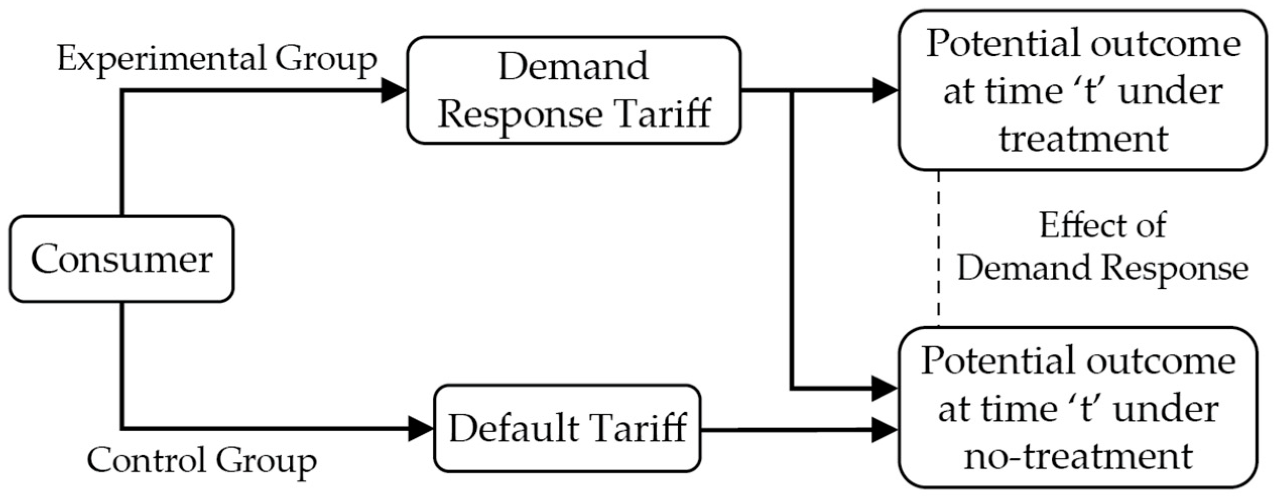
The purpose of this work was to determine the consumer consumption elasticity during the trial period and whether the dynamic tariffs offered by the DR program acted according to the objectives and took full potential of their contracted consumers. In order to estimate consumption elasticity, most experiments will rely on using two groups that are identical in most ways except that one receives a treatment while the other does not. All consumers would be subject to the estimation process with some of them selected as under treatment while some are under no treatment, as shown in Figure 1. The experiments are performed with these two sets of consumers at the same time, one of them corresponding to the control group and the other to the experimental group. However, this sometimes tends to be more expensive and time consuming, with both the control and experimental groups having the need to be closely similar in most aspects of consumption. The other way is to use observational methods and try to understand the causal effects in the absence of an experiment.

A causal inference approach was used to identify a specific set of consumer sub-groups within the DR residential clients who would respond to a specific DR period. This data-driven approach involves a methodology in which the retailer analyzes the consumption pattern of the consumers before and after the intervention of the DR program. This helps in identifying whether the consumer has performed the DR action during the contracted DR periods. Based on these computations, the elasticity of each consumer is obtained to provide the weight (or rank) for their DR response. The accumulated weight identifies the most reliable (highly responsive) group of contracted clients for a specific DR strategy.

The proposed model is detailed in Figure 2 and it examines the consumer’s DR behavior. This is done by using data-driven algorithms, which explore both machine learning and causal inference techniques in order to build a model to estimate the elasticity of the consumers. The retailer sets the DR strategy, which is then sent periodically to the contracted clients. The behavior of each consumer to the DR signals is recorded via home automation systems and this feedback is used to understand their actual behavior elasticity. The client consumption, associated DR price (€/kWh), and time components are the features fed into the causal inference model. The average consumption and elasticity for each hour is computed and ranked to identify the best set of clients. Knowing the average elasticity is more important than identifying sporadic highest and lowest consumptions, as this gives a more consistent response behavior.

The modeled approach helps in making a fair estimate of whether the consumer introduced any changes to their consumption based on DR signals, as it can differentiate between a normal consumption and a DR stimulated consumption. The consumption elasticity will give the approximate average range a consumer is willing to change in their consumption. This will help identify whether the client is more willing or reluctant to alter their consumption at that period. This result will be more of a percentage of willingness to participate or predicted to participate in a given DR activity, rather than a hard yes or no to a given signal. This could lead us to a gateway to identify how willing a particular client is, and how this willingness can be influenced to get the maximum benefits for both the client and the retailer.

2.2.2. Causality Inference Algorithms

Data analysis and causal inference for our framework was performed by two separate algorithms, one based on Robin’s G-method and the other using Bayesian structural time-series model. The first algorithm used in our consumer elasticity model uses the parametric g-formula (as the causal effect estimator) and arbitrary machine learning estimators to analyze and plot causal effects [29]. Causal effect refers to the distribution or conditional expectation of Y given X, controlling for an admissible set of covariates, Z, to make the effect identifiable. In our analysis (simple depiction in Figure 3), X, being price, and Z, being time, are indeed correlated; more precisely, they will be statistically dependent. This is basically a fork graph showing that X and Y are related with a common cause, Z. It should be noted that it is necessary for variable Z to satisfy the back-door criterion, meaning that it should block all backdoor paths from treatment to the outcome variable and it should not include any descendants of the treatment variable [30]. If Z satisfies this back-door criterion, then the effect of X on Y can be shown as Equation (1), which provides the distribution of Y.

$$P\left(Y|do\left(X=x\right)\right)={{\displaystyle \sum }}_{Z}P\left(Y|X,Z\right)P\left(Z\right),$$

(1)

$$E\left(Y|x\right)={{\displaystyle \sum }}_{Y}YP\left(Y|x\right)= {{\displaystyle \sum }}_{Y,Z}YP\left(Y|X,Z\right)P\left(Z\right),$$

$$E\left[Y|do\left(X=x\right)\right]={{\displaystyle \sum }}_{Z}E\left[Y|X,Z\right]P\left(Z\right),$$

(2)

$$E\left[Y|\left(X_j\right)\right]={\displaystyle \sum }_{h=1}^{24}\frac{1}{N}{\displaystyle \sum }_{i=1}^{N}E\left[Y|X_j,(Z_{hi}, Z_{2i}, Z_{3i})\right]$$

(3)

$$Z-Interval= E\left[Y|X,Z\right]\pm z_{\alpha /2}\left(\sigma \right)$$

(4)

The Robin g-method enables the identification and estimation of the effects of generalized treatment, exposure, and intervention plans. It provides consistent estimates of contrasts of average potential outcomes under a less restrictive set of identification conditions than standard regression models [31]. The model used by the default to minimize the mean-squared error and do the controlling is a Kernel regression model, which gives us the conditional expectation as shown in Equation (2). The causal dataframe helps in finding the true dependency between the X (price) and Y (consumption) with the confounders as the calendar variables, we consider X: Price, Y: Consumption, and Z: Calendar variables (hour—Z₁, day—Z₂, and week—Z₃). For every hour (Z₁), the causal effect of (X) on (Y) is obtained for each DR price (X_j) with a constant (Z₁) and variable (Z₂ and Z₃) with i = 1 to N running over all data points as shown in Equation (3). These calendar variables are confounders that have effects on both price and consumption. The causal analysis model works by controlling the Z variables when trying to estimate the effect of variable X on a continuous variable Y, as shown in Equation (3). The model returns Y estimates (E[y]) at each X = x value for every Z and provides the upper and lower average consumption limits of the Y variable, which is used to determine the average elasticity. The upper and the lower consumption limits of the average Y variable (for each price) is the z-intervals calculated using the confidence levels (CI = 95% for our model). The z-interval for our consumption average Y estimates is shown in Equation (4), where $z_{\alpha /2}$ is the alpha level’s z-score for a two tailed test (based on the value of CI) and $\mathsf{\sigma }$ is the standard deviation of our average Y estimate. The constructed causality model is then used to provide the estimates for each consumer demand on each hour for each price. The parametric g-formula is implemented using python library Causality [32].

The Bayesian structural time-series model is used to determine the extent to which the price change affects a consumer’s electricity consumption (i.e., the probability of the price having a causal effect on consumption) [33]. This causal analysis is used for comparison and validation of the results obtained from the Robin g-model. This package performs causal inference through counterfactual predictions using a Bayesian structural time-series model. The model requires a set of control time series (the time before the intervention—pre-period) and a set of response time series (the time from the beginning of intervention until it ends—post-period). With these two sets of time defined datasets, the package constructs a Bayesian structural time-series model and predicts how the response would have evolved if the intervention had never occurred (counterfactual prediction). As this is a non-experimental approach to estimate causal effects, conclusions require assumptions to facilitate accuracy. The model assumes that:

• There is a set control time series (pre-period) that is itself not affected by the intervention. If they were, it might falsely under or overestimate the true effect. Or it might falsely conclude that there was an effect even though in reality there was no effect.
• The relationship between covariates and the treated time series, as established during the pre-period, remains stable throughout the post-period.
• The relationship between the covariates (the time components) and the treated time series (electricity consumption) remains stable throughout the post-period.

If the posterior tail-area probability is very low, the chances of having a positive effect from the intervention is significant. This probability is obtained by calculating the posterior distribution of the response variable (Y—consumer electricity consumption) that would be expected in the absence of an intervention. The actual observed response is then compared to this posterior distribution. The tail-area probability is the probability under the calculated posterior that the response is at least as extreme (away from the expected value) as the observed one. The Bayesian structural time-series model is implemented using the CausalImpact R package [34].

Both algorithms mentioned above are fed with half hour electricity consumption data and price signals (time-of-use retail rates) from the LCL dataset, and hourly electricity consumption data along with their CPP signals, electric vehicle consumption, and solar rooftop production from the Pecan Street dataset. The time components, such as hour, day, week season, etc., have a higher degree of influence on a consumer’s load demand. This is evident from the daily average demand curve for residential consumers. The influence of time on the DR tariff is also evident, such as higher demand periods occurring during mornings or late evening, resulting in possible peak load pricing. Thus, for our analysis, we considered time components as our confounder. Both the datasets are modified to include calendar variables, which act as our confounders that can be controlled for estimating the causal effect of the DR tariffs on consumption profiles for each hour. It should be noted that both these algorithms are only fed with consumer time-series data that experiences demand response signals with no inclusion of a control group. This makes our model more unique to include any DR dataset with just the pre-period and post-period consumption behavior along with their confounders for a single set of consumers experiencing any type of DR tariff.

3. Results and Discussion

3.1. Low Carbon London (LCL) Dataset

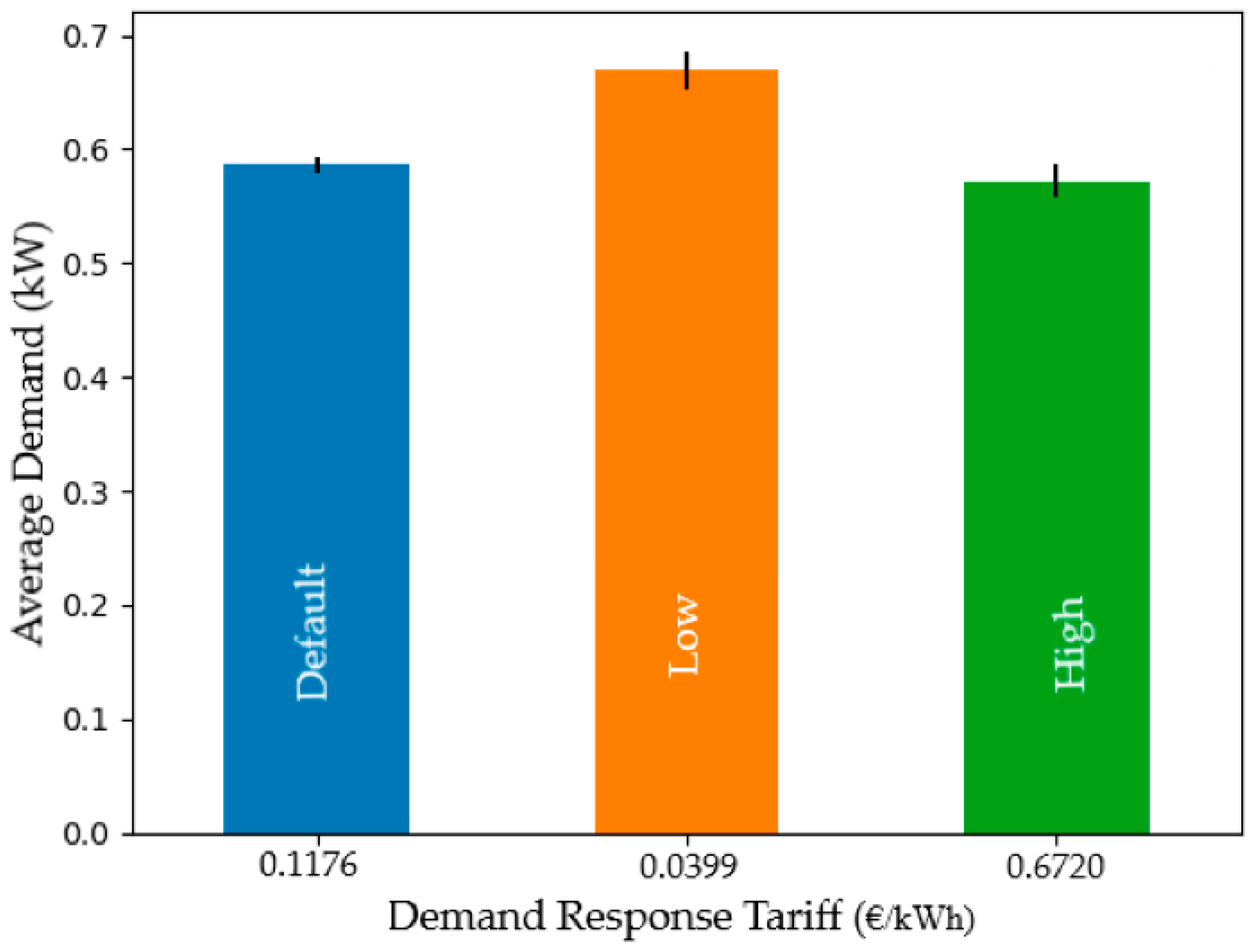
Considering the three pricing tariffs adopted in the LCL dataset, the average elasticity for the default price is expected to be low and the only elastic consumption pattern that can be observed is between periods of consumption (morning, afternoon, evening, and night) and between weekday and weekend consumption. Figure 4 indicates the average consumption for a DR client with their average consumption elasticity (indicated by the vertical black lines on top of each bar) for each price they experience. There is a clear evidence that experiencing a lower price tariff increases the average consumption along with the elasticity, whereas the default tariff sees marginal elasticity in the consumption pattern. This provides a basic understanding of how this client has reacted to the DR prices, but to get more insightful information on the change in daily consumption patterns due to price changes, the analysis was conducted under disaggregated hourly average consumption and elasticity. Figure 5a,b gives a clear perspective of which hours the clients prefer to actively participate in the DR program.

The general expectation is for consumers to have higher average consumption for lower tariff and lower average consumption for higher tariff periods (i.e., for an ideal client, one would expect, a high elastic and high average consumption for a low price (0.0399 €/kWh) and high elasticity and low average consumption for a high price (0.6720 €/kWh)). This could give an insight into how the clients will respond to DR signals, and some periods where the consumers respond poorly for a broader time interval. Thus, the higher the average elasticity for the client for those hours, the higher their tendency is to alter consumption for those price signals in those hours. Lower elasticity means that the client is not susceptible to change its consumption in those hours. (Note: Change in consumption indicates an increase or decrease during lower (L) or higher (H) price periods).

The actual average demand (blue, orange, and green bars in Figure 4) gives a sense of average consumption levels associated to each client for each price signal they experience. When all consumption averages of a client are close to each other, it signifies that the client does not have much elasticity between different price tariffs. This is evident during the early periods from 0 h until 7 h for the considered client from Figure 5a. This specific client shows more flexibility in its consumption between 8 and 17 h, where its average is lower for a high price and higher for a lower priced tariff. The elasticity for lower price and higher price tariffs trades places during early evening and at night, which corresponds to the number of high and low prices actively experienced by the consumer during those hours. Figure 5b shows the average elasticity values that were obtained for consumer D0641 and indicates which hours are preferred by this client to change its consumption pattern based on the prices experienced. Comparing the average elasticity plot and the average consumption plot, we can clearly see that this client willingly participates in the DR activity, specifically during the morning and evening periods. They also exhibit low price consumption elasticity during the afternoon.

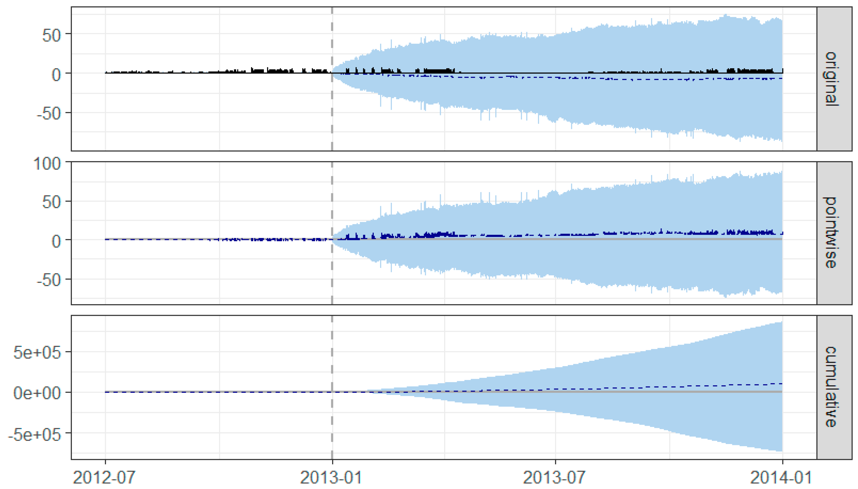
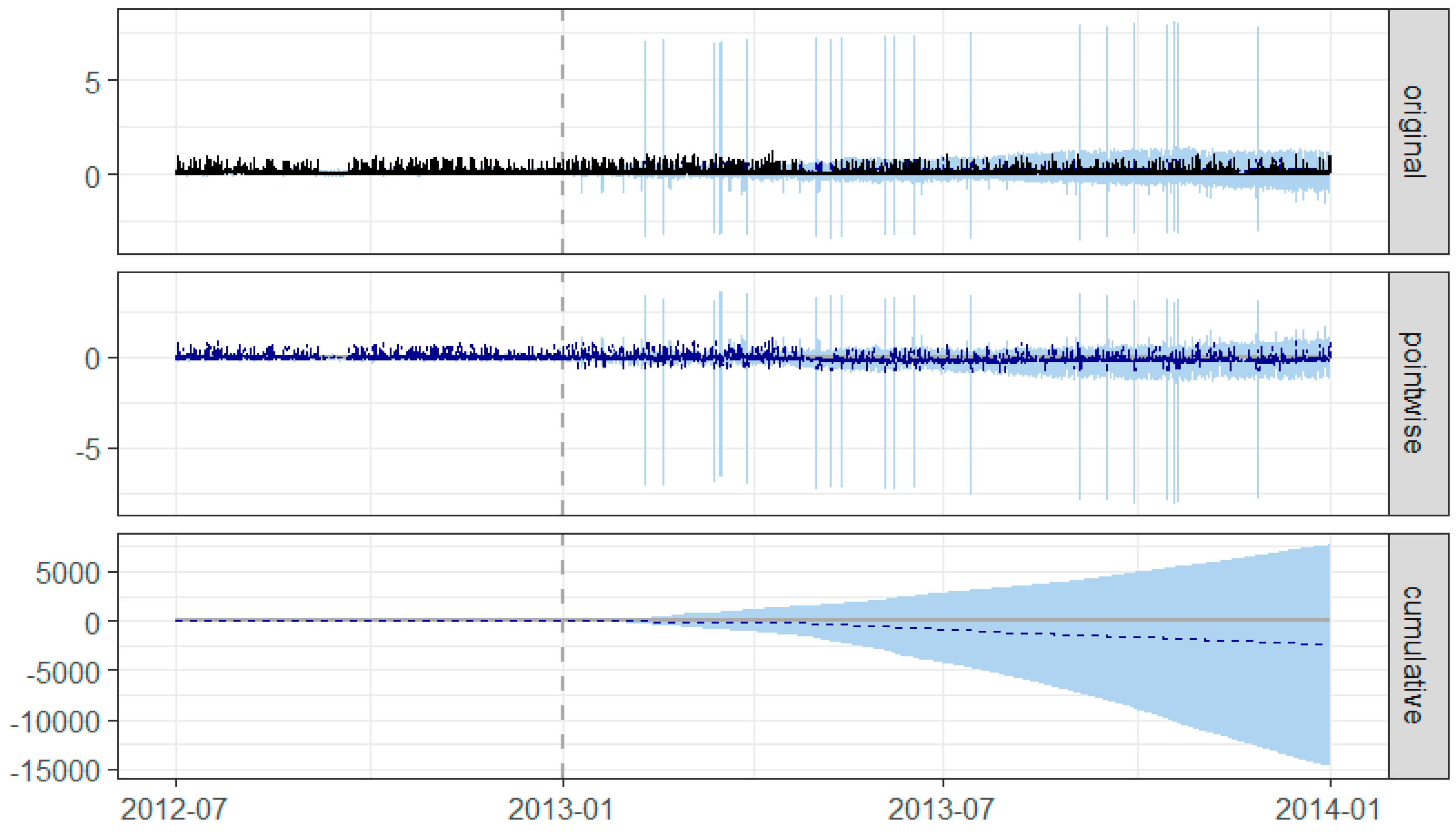
Figure 6 shows the posterior distribution for the causal effect obtained from the Bayesian structural time-series model for the same consumer D0641. The original time-series plot shows the black lines of what happened before and after intervention (from January 2013) along with the prediction of what might have happened in the absence of intervention. The pointwise plot shows the difference between the observed data and the counterfactual estimates and the final time-series showing the accumulated causal effect over time. The posterior probability distribution of the response variable in the absence of intervention (counterfactual time-series) was computed using the time-series behavior of the response variable prior to intervention. The 95% confidence interval for this distribution indicates that predictions should become increasingly uncertain as we move along the time-series. From the analysis, we can confirm that this client has actively responded to DR signals. Figure 7a,b shows the actual average consumption and average consumption elasticity of another client (consumer D0421), who has a much lesser elasticity compared to the rest of the pool of clients. Even though the developed model picks up average consumption changes, the magnitude of the consumption elasticity is too small to have any kind of meaningful impact in the overall DR event. This inference is backed by the statistical R result (Figure 8), which shows a narrow posterior probability interval, suggesting that the prediction uncertainty is less.

As mentioned initially, one of the aims of this work was to cluster the consumers together into weighted categories, ranking their acceptance to each DR event. To determine the best set of DR consumers amongst all for each hour, the elasticity of each consumer was ranked per hour. The rank computed (between 0–100) for each of these clients on their elasticity was compared against all the 81 clients in the pool and sorted to give the best and the worst. Figure 9 and Figure 10 depict the obtained ranks for the low and the high price levels, in which an increasing value from 0 to 81 means an increased elasticity. A specific client, who has a higher rank for a few hours, may not have the best rank for the rest of the hours. The result provides the overall consistent consumers between all the consumers and ranks them on a 24 h space. This ranking will certainly differ, when considering each hour. It could also be used to find the client that has the best response over the entire period of DR evaluation. This gives an insight into consistent clients who have participated in most of the DR signal calls and have changed their consumption accordingly. Thus, we formed an effective system to sort the clients according to their rank that provides the list of the most consistent and the least consistent clients in the pool for each pricing level in the DR tariff. One can notice that many consumers in the mid table of Figure 9 and Figure 10 exhibit a higher consumption elasticity than the rest of the periods during the day. This is particularly due to the availability of consumers during these day periods (especially during morning and evening hours) in their house to actively perform consumption changes. This is also evident form our result in Figure 5a for client D0641.

From the Bayesian structural time-series model, the difference between observed data and counterfactual predictions is the inferred causal impact of the intervention. Figure 11 gives a description of this inferred causal impact along with the probability of occurrence of such an impact by the consumers. Consumers D0767, D0323, and D0486 exhibit changes in their average consumption change while consumers D0328 and D0026 exhibit zero change, indicating that they did not effectively participate in the DR program. This validates the observations from the Robin g-method results as shown in Figure 9 and Figure 10.

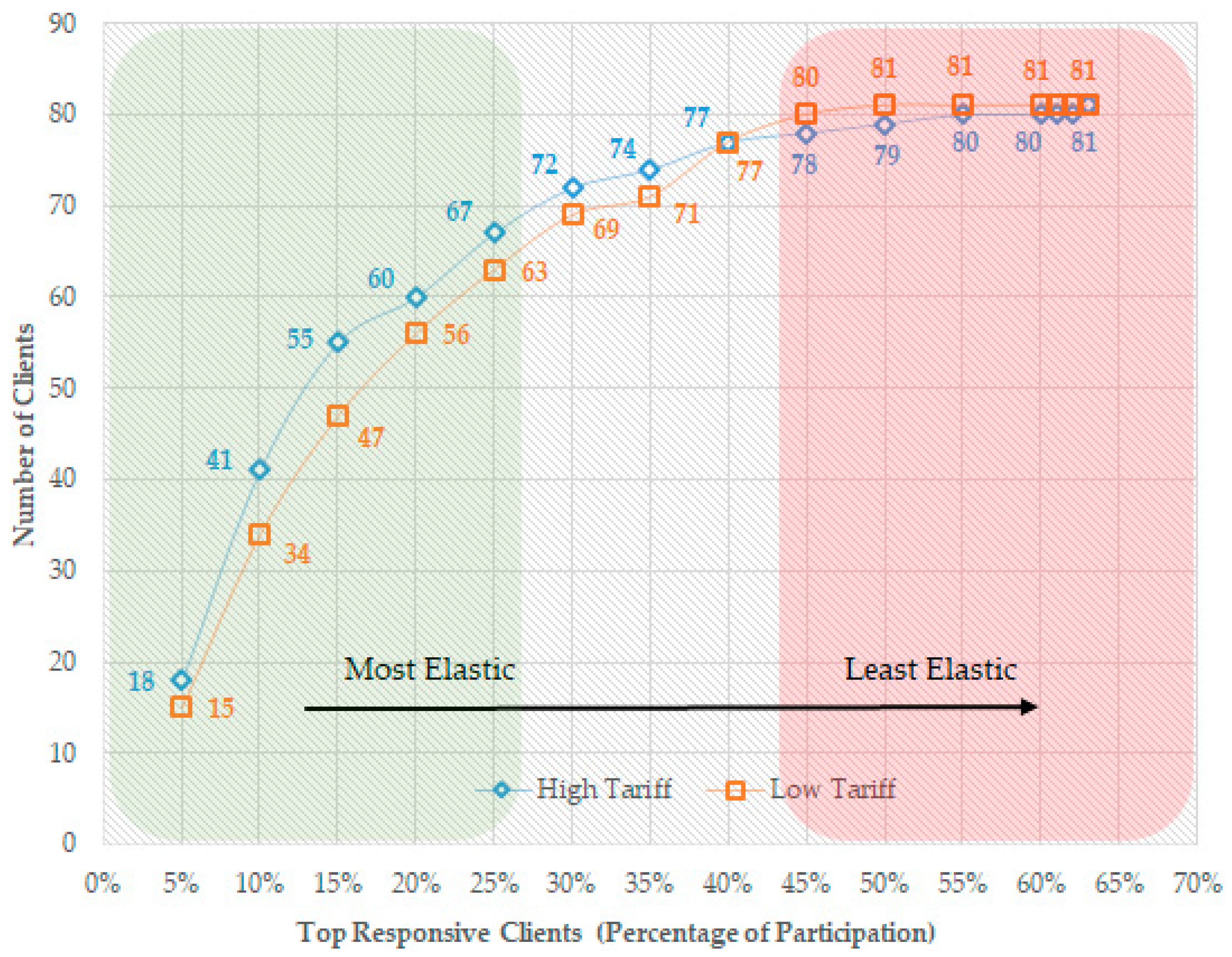
The python elasticity model is used as a performance measure to rate the quality of the DR strategy and the effect it has on the contracted clients. A DR program can be considered effective when all its contracted clients are actively participating in a consistent manner. By accumulating the ranks of each client between the 81 clients for each period, we can find the top (5%, 10%, …, 50%, etc.) actively participating clients. Using these metrics, we can find the number of clients in the top percentage levels as shown in Figure 12. Amongst the top 5% actively participating clients, there are 15 and 18 clients, respectively, for low price and high price. This graph shows that when the percentage of participation is relaxed to around 63%, all 81 consumers in the pool have at least participated once in a DR event. This indicates that the DR program has not been able to benefit from all their clients effectively. The goal of the retailer would be to increase the most elastic region to improve their reliability in providing the DR service to the market and increase its profit margin by selling system services to system operators. By ranking the consumers in terms of their consumption elasticity, the retailer can design a financial and marketing strategy to maintain consumers with high elasticity and attract new ones so that the elastic region is increased. Furthermore, with causality inference, it is also possible to trial different DR products and assess consumers’ responsiveness to improve the design of dynamic tariffs in order to maximize elasticity in different hours/periods. The retailer will have the ability to look into each hour and request or check a specific elasticity level. This allows the retailer to make an informed decision on how much DR will be available for it during a particular period with greater accuracy, make better bids in the market with little to no penalty incurred, and provide better network reliability. An ideal strategy for a retailer could be to have bigger elastic region and higher service reliability to win more bids and get higher profits.

3.2. Pecan Street Inc. Dataset

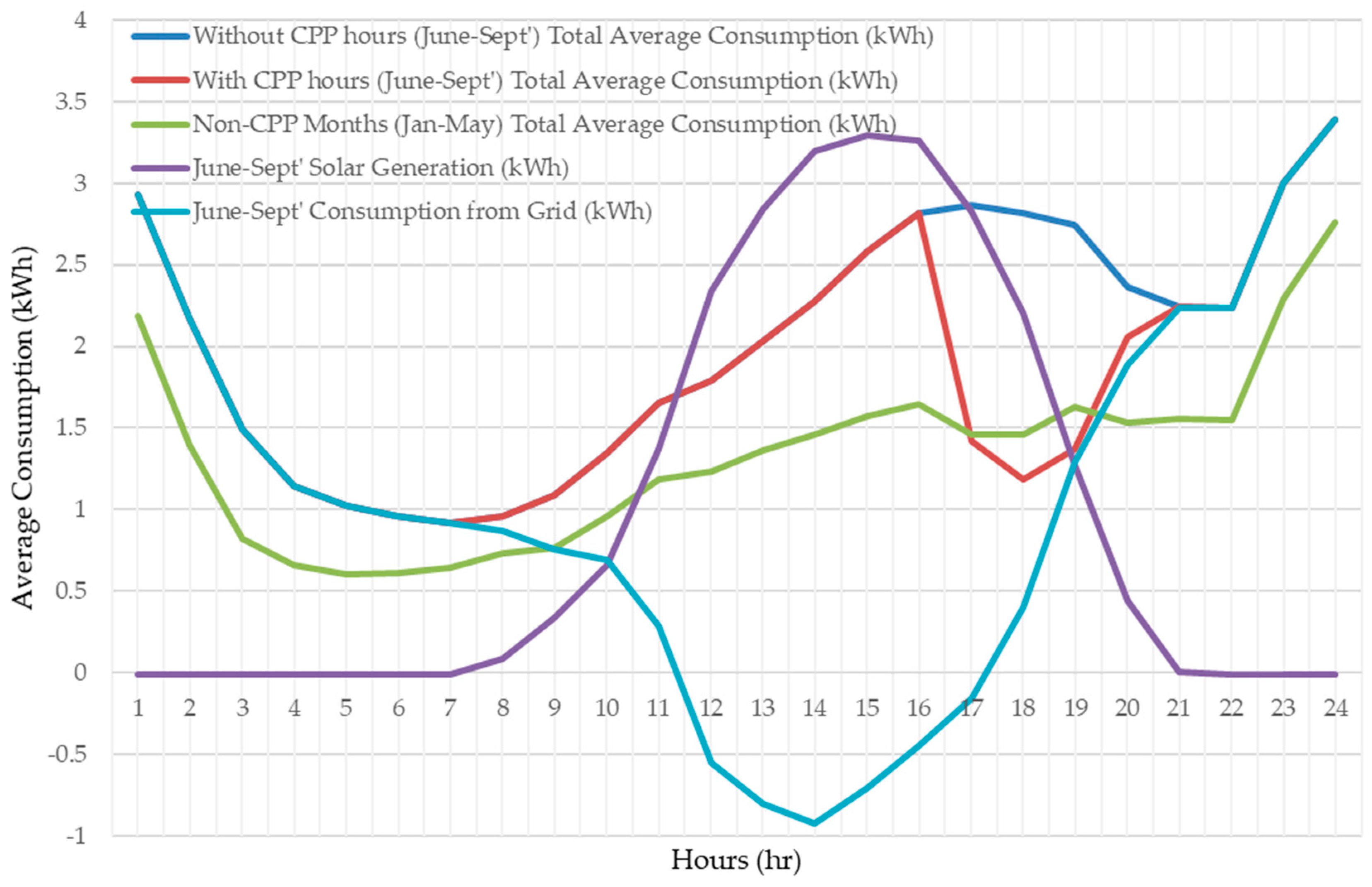
The CPP DR strategy was conducted during the peak summer days for the months June to September. The group of residents in the Austin, Texas region were expected to shift their demand when the ERCOT electric grid in Texas was experiencing demand-driven strains during high peak periods. It should also be noted that consumers from this trial were also equipped with solar rooftops and electric vehicles. These play a major role in understanding how the consumers’ consumption is influenced by price incentives apart from the available devices that they can use for this purpose. As the CPP events were conducted separately in 2013 and 2014, we aimed to identify the consumption elasticity and average separately for both these years to see if the program had better influence in the second year due to the experience gained by the consumer in the first year. The general expectation for a CPP incentivized DR program is to have a lower average electricity consumption during high price CPP periods and shift this demand effectively to the non-peak periods.

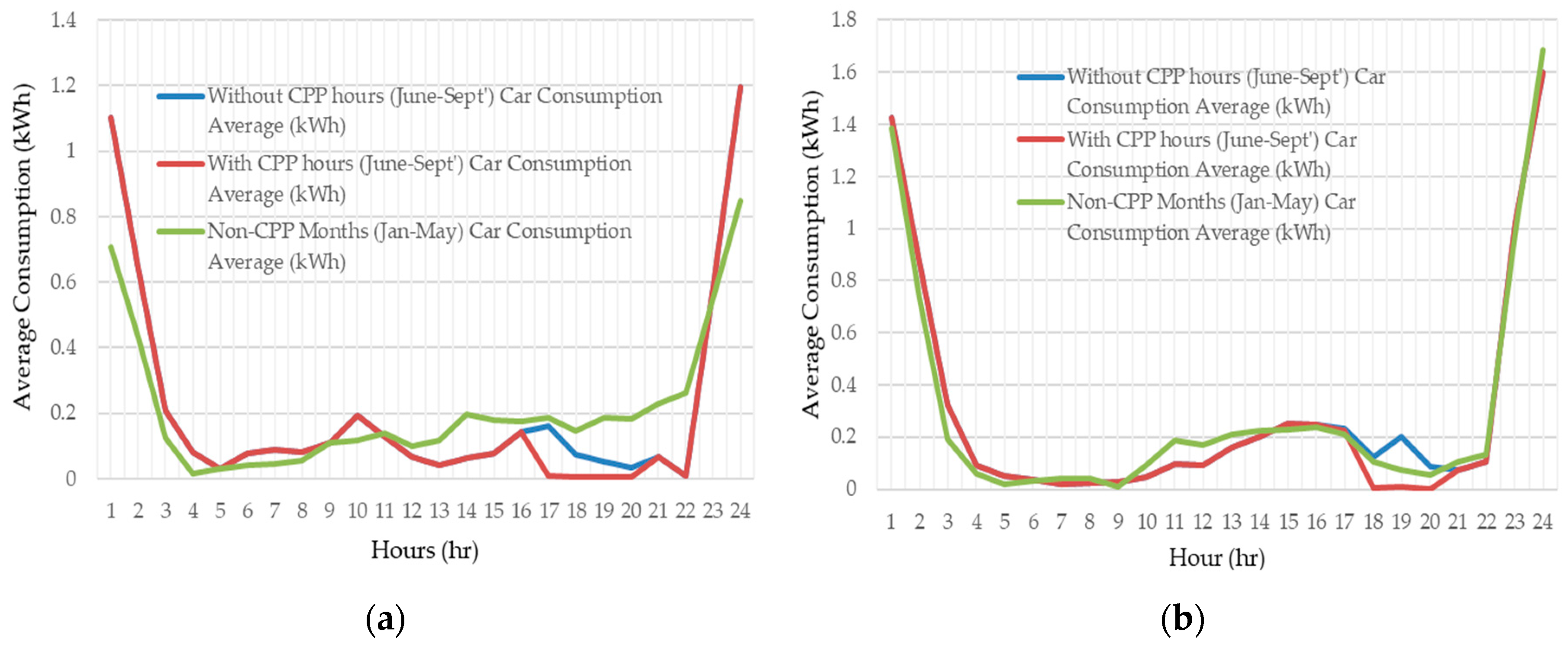
Figure 13 and Figure 14 give the disaggregated hourly average consumptions for consumer 370 over the years 2013 and 2014. As expected, there is a clear evidence that CPP periods experienced during the evening hours (16–19 h) show a reduced average consumption than those of the same, with non-CPP hours during the same months of June to September. This indicates that this particular consumer was responsive to the DR signals in the first year of participation (2013). It has to be noted that this consumer’s overall average consumption during the non-CPP hours during the months of June to September increased from the non-CPP month’s average (shown in green). On the positive note, we understand that the DR program encouraged this consumer to reduce his overall average consumption in 2014, as seen in Figure 14. This reduced average demand in 2014 also resulted in more consumption from solar generation, specifically during the hours before and during the CPP period. Figure 15 describes the average charging profile of the electric vehicle (EV) owned by consumer 370. Comparing 2013 and 2014, the consumer seems to have had completely lowered their EV demand in 2013 during the day and shifted their demand to the night periods. Whereas, in 2014, they were inelastic to the CPP signals in regards to EV charging. This shows that they preferred the comfort of having their EV charged regardless of the price change.

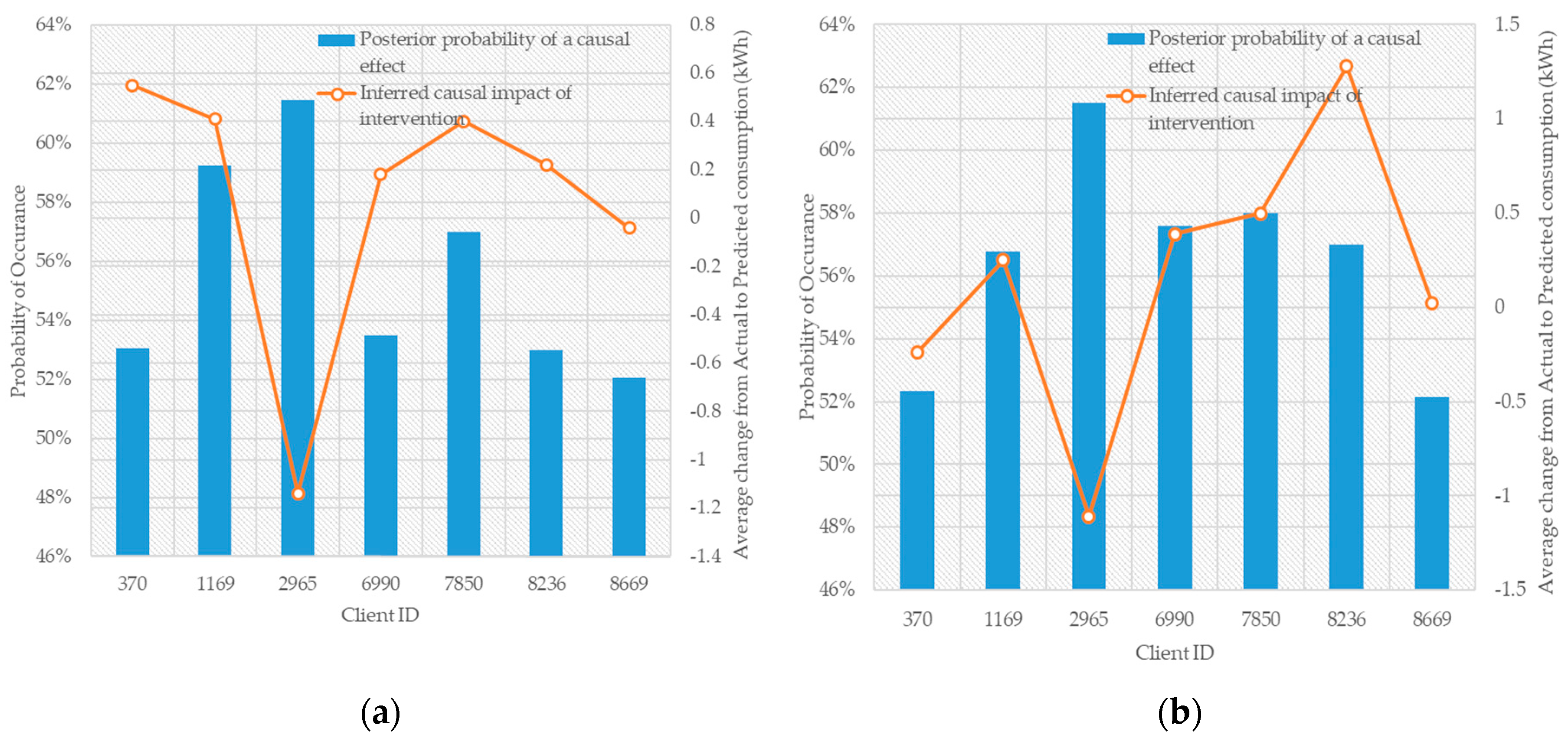
The difference in consumption elasticity (Figure 16) between 2013 and 2014 is due to their reduction in the total average consumption during the CPP period in 2014. Figure 16b also shows that the consumer exhibits consumption elasticity even in the non-CPP months (January–May 2014) as the influence of the first CPP program in 2013 (in 2013, this curve was flatter, indicating little to no elasticity during non-CPP months). This is an indication that our model picks up elasticity profiles even after the CPP months have ended and how that influences the normal consumption of the consumer with a default tariff. This is an important identification as one can determine the effect a DR program has made on a consumer even after the program has ended. In 2014, the non-CPP months having a very similar elasticity profile to that of the CPP months indicates that the consumer is closer to the maximum elasticity they can provide without sacrificing more of their comfort. This is an indication that the CPP program effectively encouraged this consumer to reduce its consumption during the CPP months in the second year of enrolment. Figure 17 shows the posterior distribution for the causal effect obtained from the Bayesian time-series model for the same consumer. As explained in the previous section, the progressive widening of the posterior intervals (95% posterior probability intervals) indicates that predictions should become increasingly uncertain as we move along the time-series. This is evident with the results obtained from the Bayesian time-series model (Figure 17 and Figure 18), which gives us the inferred causal impact along with the probability of occurrence. Figure 18 describes the inferred causal impact along with the probability of occurrence of such an impact by the consumer. In 2013, consumers 370, 1169, and 7850 exhibit changes in their average consumption (indicating reliable consumption elasticity) while consumers 2965, 6990, 8236, and 8669 exhibit little to no elasticity in their average consumption. This, compared with 2014, shows the saturation level of elasticity for consumer 370, while consumer 8236 exhibits more elasticity compared to their 2013 behavior. Consumer 8669 indicates no real interest in modifying their average consumption, indicating that they are not very reliable in actively participating in DR activity.

4. Conclusions

Studies on consumer behavior towards DR are quite new and most of them are quantitative analysis. One should note that in a general household scenario, day-to-day energy consumption activities are performed habitually with little, if any, conscious awareness of their impacts. Because of such habitual behaviors, successful interventions are required to instigate household consumers to make physical, material, or behavioral activity change in their house to promote DR. With many DR incentives currently in use, our study focused on tariffs and how they bring about change in residential consumers’ electricity consumption behavior.

From our analysis of the LCL dataset, it was observed that price changes do not always lead to the best outcome for retailers (only a small portion of consumers seem to actively participate in DR signals). We inferred whether the consumers who accepted the DR signals have done so purely based on the financial benefits they received due to the price change, or if they preferred comfort rather than being flexible to the tariff. This is understood by clustering (grouped) sets of consumers according to their responses. The higher ranked consumer is more susceptible to accept price incentives than the lower ranked consumer, who prefer offers that meet their comfort zones. This leads to a way to performance-based payments for residential DR clients, i.e., payments to those clients who actively participate in the DR signals they receive. From our work with the Pecan Street Inc. dataset, we were able to identify if the critical peak pricing strategy had desirable impacts on consumers. It was observed that many consumers tend to exhibit increased baseline consumption during the DR months in the first year (which undermines their observed consumption elasticity) of involvement but tend to provide more consumption elasticity and reduced average consumption in the second year, making them more reliable for the CPP demand response.

The approach reported in this paper can be used to provide a clear picture to the retailers in terms of the impact DR offers make on a specific client, i.e., if the tariff is lower or increases twice for a given period, how a client would react to such variations. Our approach using causal inference will identify the best DR strategies to which all-individual contracted DR clients would actively participate in. It groups consumers for a specific set of DR events, thus enhancing the success rate of DR, and paves a way for performance-based payments for residential DR clients. The ideal plan would be to make each of these clustered DR hours dense so that more contracted consumers fit into almost all the DR strategy periods, thus increasing the robustness and effectiveness of the DR program. The designed model can be generalized to use any type of DR tariff (as we have seen in the use of TOU and CPP tariffs in our study). The performance measure plot and consumer ranking can be used to identify why and for whom the DR signals are unsatisfactory and address those issues accordingly or at least make a way for each of them to participate in as many DR periods as possible. This idea will be extended to estimate the level to which the retailer can effectively help to smooth the cumulative demand curve. Further, we will determine the bill savings the consumer can expect from actively participating in these DR programs.

References

- Siano, P. Demand response and smart grids-A survey. Renew. Sustain. Energy Rev. 2014, 30, 461–478. [Google Scholar] [CrossRef]
- Zhu, X.; Li, L.; Zhou, K.; Zhang, X.; Yang, S. A meta-analysis on the price elasticity and income elasticity of residential electricity demand. J. Clean. Prod. 2018, 201, 169–177. [Google Scholar] [CrossRef]
- Hesser, T.; Succar, S. Renewables Integration Through Direct Load Control and Demand Response. Smart Grid 2012. [Google Scholar] [CrossRef]
- Herter, K. Residential implementation of critical-peak pricing of electricity. Energy Policy 2007, 35, 2121–2130. [Google Scholar] [CrossRef] [Green Version]
- Ruiz, N.; Cobelo, I.; Oyarzabal, J. A direct load control model for virtual power plant management. IEEE Trans. Power Syst. 2009, 24, 959–966. [Google Scholar] [CrossRef]
- Mohsenian-Rad, A.H.; Leon-Garcia, A. Optimal residential load control with price prediction in real-time electricity pricing environments. IEEE Trans. Smart Grid 2010, 1, 120–133. [Google Scholar] [CrossRef]
- Belgium, C. Impact Assessment Support Study on Downstream Flexibility, Demand Response and Smart Metering; European Commission: Brussels, Belgium, 2016. [Google Scholar]
- Observation, G.; Algorithms, R.; Gas, S.F.-B.P.; Holding, E. Assessment of Demand Response and Advanced Metering Staff Report Federal Energy Regulatory Commission; Federal Energy Regulatory Commission: Washington, DC, USA, 2002; pp. 2–5.
- Puget Sound Energy (PSE). Request for Proposals (RFP)-Technology and Implementation Services-Direct Load Control Program; Puget Sound Energy (PSE): Bellevue, WA, USA, 2016. [Google Scholar]
- Bertoldi, P.; Zancanella, P.; Boza-Kiss, B. Demand Response Status in EU Member States; European Union: Brussels, Belgium, 2016; pp. 1–153. [Google Scholar]
- Anca-Diana Barbu, N.G.; Morton, G. Achieving Energy Efficiency through Behaviour Change What Does it Take; European Environment Agency and Ricardo-AEA: Luxembourg, 2013. [Google Scholar]
- Hassan, N.; Pasha, M.; Yuen, C.; Huang, S.; Wang, X. Impact of Scheduling Flexibility on Demand Profile Flatness and User Inconvenience in Residential Smart Grid System. Energies 2013, 6, 6608–6635. [Google Scholar] [CrossRef]
- Asadinejad, A.; Rahimpour, A.; Tomsovic, K.; Qi, H.; Chen, C.-F. Evaluation of residential customer elasticity for incentive based demand response programs. Electr. Power Syst. Res. 2018, 158, 26–36. [Google Scholar] [CrossRef]
- Klaassen, E.A.M.; Kobus, C.B.A.; Frunt, J.; Slootweg, J.G. Responsiveness of residential electricity demand to dynamic tariffs: Experiences from a large field test in the Netherlands. Appl. Energy 2016, 183, 1065–1074. [Google Scholar] [CrossRef] [Green Version]
- Baker, P.; Blundell, R.; Micklewright, J. Modelling Household Energy Expenditures Using Micro-Data. Econ. J. 2006, 99, 720. [Google Scholar] [CrossRef]
- Kamerschen, D.R.; Porter, D.V. The demand for residential, industrial and total electricity, 1973–1998. Energy Econ. 2004, 26, 87–100. [Google Scholar] [CrossRef]
- Schleich, J.; Klobasa, M.; Gölz, S.; Brunner, M. Effects of feedback on residential electricity demand-findings from a field trial in Austria. Energy Policy 2013, 61, 1097–1106. [Google Scholar] [CrossRef]
- Zhou, D.; Balandat, M.; Tomlin, C. Residential demand response targeting using machine learning with observational data. In Proceedings of the 2016 IEEE 55th Conference on Decision and Control, Las Vegas, NV, USA, 12–14 December 2016; pp. 6663–6668. [Google Scholar]
- Kravitz, R. Distributed Energy Resources, SCE Slides for California Energy Commission; California Energy Commission: Sacramento, CA, USA, 2017.
- Larsen, E.M.; Pinson, P.; Leimgruber, F.; Judex, F. Demand response evaluation and forecasting—Methods and results from the EcoGrid EU experiment. Sustain. Energy Grids Netw. 2017, 10, 75–83. [Google Scholar] [CrossRef]
- Ray, G.L.; Larsen, E.M.; Pinson, P. Evaluating Price-Based Demand Response in Practice—With Application to the EcoGrid EU Experiment. IEEE Trans. Smart Grid 2018, 9, 2304–2313. [Google Scholar]
- Kwac, J.; Rajagopal, R. Data-driven targeting of customers for demand response. IEEE Trans. Smart Grid 2016, 7, 2199–2207. [Google Scholar] [CrossRef]
- Behl, M.; Smarra, F.; Mangharam, R. DR-Advisor: A data-driven demand response recommender system. Appl. Energy 2016, 170, 30–46. [Google Scholar] [CrossRef] [Green Version]
- Fotouhi Ghazvini, M.A.; Soares, J.; Morais, H.; Castro, R.; Vale, Z. Dynamic Pricing for Demand Response Considering Market Price Uncertainty. Energies 2017, 10, 1245. [Google Scholar] [CrossRef]
- Schofield, J.R.; Carmichael, R.; Schofield, J.R.; Tindemans, S.H.; Bilton, M.; Woolf, M.; Strbac, G. Low Carbon London Project: Data from the Dynamic Time-of-Use Electricity Pricing Trial; UK Data Service: Colchester, UK, 2013; p. 7857. [Google Scholar]
- Weather Underground Historic Weather Data. 2014. Available online: https://www.wunderground.com/history/ (accessed on 5 August 2018).
- Pecan Street Inc. Pecan Street Dataport. 2018. Available online: https://dataport.pecanstreet.org/ (accessed on 23 July 2018).
- Rhodes, J.D.; Upshaw, C.R.; Harris, C.B.; Meehan, C.M.; Walling, D.A.; Navrátil, P.A.; Beck, A.L.; Nagasawa, K.; Fares, R.L.; Cole, W.J.; et al. Experimental and data collection methods for a large-scale smart grid deployment: Methods and first results. Energy 2014, 65, 462–471. [Google Scholar] [CrossRef]
- Keil, A.P.; Edwards, J.K.; Richardson, D.B.; Naimi, A.I.; Cole, S.R. The parametric g-formula for time-to-event data: intuition and a worked example. Epidemiology 2014, 25, 889–897. [Google Scholar] [CrossRef]
- Pearl, J. Causality: Models, Reasoning, and Inference; MIT Press: Cambridge, MA, USA, 2009; p. 464. [Google Scholar]
- Naimi, A.I.; Cole, S.R.; Kennedy, E.H. An introduction to g methods. Int. J. Epidemiol. 2017, 46, 756–762. [Google Scholar] [CrossRef]
- Kelleher, A. Tools for Causal Analysis. 2017. Available online: https://github.com/akelleh/causality (accessed on 5 July 2018).
- Brodersen, K.H.; Gallusser, F.; Koehler, J.; Remy, N.; Scott, S.L. Inferring causal impact using Bayesian structural time-series models. Ann. Appl. Stat. 2015, 9, 247–274. [Google Scholar] [CrossRef]
- Kay, H.; Brodersen, A.H. An R Package for Causal Inference Using Bayesian Structural Time-Series Models; Google, Inc.: Mountain View, CA, USA; GitHub: San Francisco, CA, USA, 2014–2017. [Google Scholar]
Figure 1.
Common model for determining the effect of DR products on consumer electrical energy consumption.
Figure 2.
Causality inference framework for consumer elasticity.
Figure 3.
Causal graph.
Figure 4.
Average demand for three pricing tariff and observed average demand elasticity of one consumer from the Low Carbon London (LCL) dataset.
Figure 5.
Consumer D0641 under demand response with three pricing tariffs: (a) actual average consumption from the elasticity model; (b) average consumption elasticity from the elasticity model.
Figure 6.
Causal effect using Bayesian structural time-series model for consumer D0641.
Figure 7.
Consumer D0421 under demand response with three pricing tariffs: (a) actual average consumption from the elasticity model; (b) average consumption elasticity from the elasticity model.
Figure 8.
Causal effect using Bayesian structural time-series model for consumer D0421.
Figure 9.
Ranking consumer elasticity for low price using the Robin g-method.
Figure 10.
Ranking consumer elasticity for high price using the Robin g-method.
Figure 11.
Probability of causality between dynamic tariff and electrical energy consumption.
Figure 12.
Performance Measure of the LCL DR program showing active DR clients based on the percentage of participation.
Figure 13.
Actual average consumption of consumer 370 under the CPP-DR tariff for 2013.
Figure 14.
Actual average consumption of consumer 370 under the CPP-DR tariff for 2014.
Figure 15.
Average car consumption of consumer 370 under the CPP tariff: (a) 2013; (b) 2014.
Figure 16.
Average consumption elasticity of consumer 370 under the CPP tariff: (a) 2013; (b) 2014.
Figure 17.
Inferring causal impact through counterfactual predictions for consumer D0328: (a) 2013; (b) 2014.
Figure 18.
Probability of causality between the dynamic tariff and electrical energy consumption: (a) 2013; (b) 2014.
© 2019 by the authors. Licensee MDPI, Basel, Switzerland. This article is an open access article distributed under the terms and conditions of the Creative Commons Attribution (CC BY) license (http://creativecommons.org/licenses/by/4.0/).
Share and Cite
MDPI and ACS Style
Ganesan, K.; Tomé Saraiva, J.; Bessa, R.J. On the Use of Causality Inference in Designing Tariffs to Implement More Effective Behavioral Demand Response Programs. Energies 2019, 12, 2666. https://doi.org/10.3390/en12142666
AMA Style
Ganesan K, Tomé Saraiva J, Bessa RJ. On the Use of Causality Inference in Designing Tariffs to Implement More Effective Behavioral Demand Response Programs. Energies. 2019; 12(14):2666. https://doi.org/10.3390/en12142666
Chicago/Turabian StyleGanesan, Kamalanathan, João Tomé Saraiva, and Ricardo J. Bessa. 2019. "On the Use of Causality Inference in Designing Tariffs to Implement More Effective Behavioral Demand Response Programs" Energies 12, no. 14: 2666. https://doi.org/10.3390/en12142666
Note that from the first issue of 2016, this journal uses article numbers instead of page numbers. See further details here.