The Optimal Energy Dispatch of Cogeneration Systems in a Liberty Market


1
Department of Electrical Engineering, National Sun Yat-Sen University, Kaohsiung 807, Taiwan
2
College of Intelligence Robot, Fuzhou Polytechnic, Fujian 350108, China
3
Department of Electrical Engineering, Cheng-Shiu University, Kaohsiung 833, Taiwan
*
Author to whom correspondence should be addressed.
Energies 2019, 12(15), 2868; https://doi.org/10.3390/en12152868
Submission received: 20 June 2019
/
Revised: 12 July 2019
/
Accepted: 20 July 2019
/
Published: 25 July 2019
(This article belongs to the Special Issue Selected Papers from IEEE ICKII 2019)
Abstract
:This paper proposes a novel approach toward solving the optimal energy dispatch of cogeneration systems under a liberty market in consideration of power transfer, cost of exhausted carbon, and the operation condition restrictions required to attain maximal profit. This paper investigates the cogeneration systems of industrial users and collects fuel consumption data and data concerning the steam output of boilers. On the basis of the relation between the fuel enthalpy and steam output, the Least Squares Support Vector Machine (LSSVM) is used to derive boiler and turbine Input/Output (I/O) operation models to provide fuel cost functions. The CO2 emission of pollutants generated by various types of units is also calculated. The objective function is formulated as a maximal profit model that includes profit from steam sold, profit from electricity sold, fuel costs, costs of exhausting carbon, wheeling costs, and water costs. By considering Time-of-Use (TOU) and carbon trading prices, the profits of a cogeneration system in different scenarios are evaluated. By integrating the Ant Colony Optimization (ACO) and Genetic Algorithm (GA), an Enhanced ACO (EACO) is proposed to come up with the most efficient model. The EACO uses a crossover and mutation mechanism to alleviate the local optimal solution problem, and to seek a system that offers an overall global solution using competition and selection procedures. Results show that these mechanisms provide a good direction for the energy trading operations of a cogeneration system. This approach also provides a better guide for operation dispatch to use in determining the benefits accounting for both cost and the environment in a liberty market.
1. Introduction
Cogeneration systems, which combine heat and power (CHP) systems, have previously been extensively applied in industry. They offer an economic strategy providing both heat and power, which can then be passed on to buyers. Cogeneration systems offer a significant advantage when it comes to consideration of environmental issues. They are used as a distributed energy source, which can simultaneously sell both thermal steam and electricity to other industries. They can also be constructed in urban areas and used as distributed energy resources in microgrids [1,2,3]. In recent decades, consolidated cogeneration solutions have been used in industrial applications [4], while cogeneration system applications continue to grow. However, more experience is required in order to achieve the most efficient and energy-saving operation of these systems. To improve the competiveness of cogeneration systems in a liberalized market, an efficient tool for achieving the optimal operation of these systems must be developed.
To date, several efficiency strategies have been developed to achieve this optimal operation [5,6,7,8,9,10,11,12,13,14,15,16,17,18,19]. Ref. [5] presented a generalized network programming (GNP) to perform the economic dispatch of electricity and steam in a cogeneration plant. Ref. [6] presented an dispatching scheme which economically transfers energy between facilities and utilities. An optimal operation of the cogeneration system is proposed, which will integrate energy into the electricity grid by using the decision-making technique [7]. Ref. [8] is used to assess the potential process of using micro-cogeneration systems based on Stirling engines. The results demonstrate that a numerical analysis of the Stirling engine can accurately indicate the operation of the actual machine. Ref. [9] used a non-linear programming with Time-of-Use (TOU) rates considered during operation. Ref. [10] presented the operation of steam turbines experiencing blades failures during peak load times of the summer months at a cogeneration plant. The author of [11] applied some possible technologies to integrate pulp and paper production within the context of a high-efficiency cogeneration system. Grey wolf optimization [12] and cuckoo search algorithms [13] are proposed to simultaneously solve the economic logistics of using a combined heat and power system. Ref. [14,15] presented the suggested economical operation of a cogeneration system under control, with resultant multi-pollutants from a fossil-fuels-based thermal energy generation. The author of [16] introduced an original framework based on identifying the characteristics of small-scale and large-scale uncertainties, whereby a comprehensive approach based on multiple time frames was formulated. Ref. [17] developed a tool for long-term optimization of cogeneration systems based on mixed integer linear-programming and a Lagrangian relation. Ref. [18] proposed an enhanced immune algorithm to solve the scheduling of cogeneration plants in a deregulated market. Ref. [19] addressed an optimal strategy for the daily energy exchange of a 22-MW combined-cycle cogeneration plant in a liberty market.
One of the key issues of a cogeneration operation is heat and power modeling. In the papers described above, pure power dispatch was a major objective. Inevitably, though, more design objectives coupled with higher constraints will have to be incorporated. The energy trading dispatch of cogeneration systems is a complicated process, especially when the solution is being sought in a world of uncertainty. Conventional methods have thus become more difficult to solve. Recently, artificial intelligence (AI) has been applied in the economic dispatch of cogeneration systems [20,21,22,23]. The strategies proposed by AI algorithms must consider computer execution efficiency and a large computing space. Conventional algorithms may be faster, but are very often limited by the problem structure, and may diverge, or lead to a local minimum. This paper therefore proposes an Enhanced Ant Colony Optimization (EACO) to solve the energy trading dispatch of cogeneration systems.
Ant Colony Optimization (ACO) applies the activity characteristics of biotic populations to search optimization problems [24,25]. When ants are foraging, they not only refer to their own information but also learn from the most efficient ants in order to correct their route. They learn and exchange their information to search for the shortest route between their colony and food sources, and pass this information on until the whole ant colony reaches optimal status. The advantages of the ACO algorithm are that individual solutions within a range of possible solutions can converge to discover the optimal solution through a small number of evolution iterations. ACO has previously been applied to the economic dispatch of power systems [26,27,28,29,30]; however, while ACO is good at global searches, the populations produced are still a dilemma. In this paper, an EACO algorithm is proposed to improve this search ability. In the EACO, the crossover and mutation mechanisms [31] are used to generate offspring equipped to escape the local optimum. This paper proposes the use of EACO to solve the energy trading dispatch of the cogeneration systems by considering the TOU rate [32]. The different carbon prices of CO2 emissions are also simulated and analyzed in the energy trading dispatch of these cogeneration systems. It can show the performance of the energy trading dispatch of the cogeneration systems to obtain the maximal profit.
2. Problem Formulation
Figure 1 shows M back pressure steam turbines, N extraction condensing steam turbines, and K high pressure steam boilers, where the high and medium pressure steam systems are connected by a common pipeline. Part of the generated electricity is supplied to the service power, and the excess electricity is sold to the power company. Input/Output (I/O) models of the boiler and turbine are described as follows.
2.1. Operation Models of Boilers
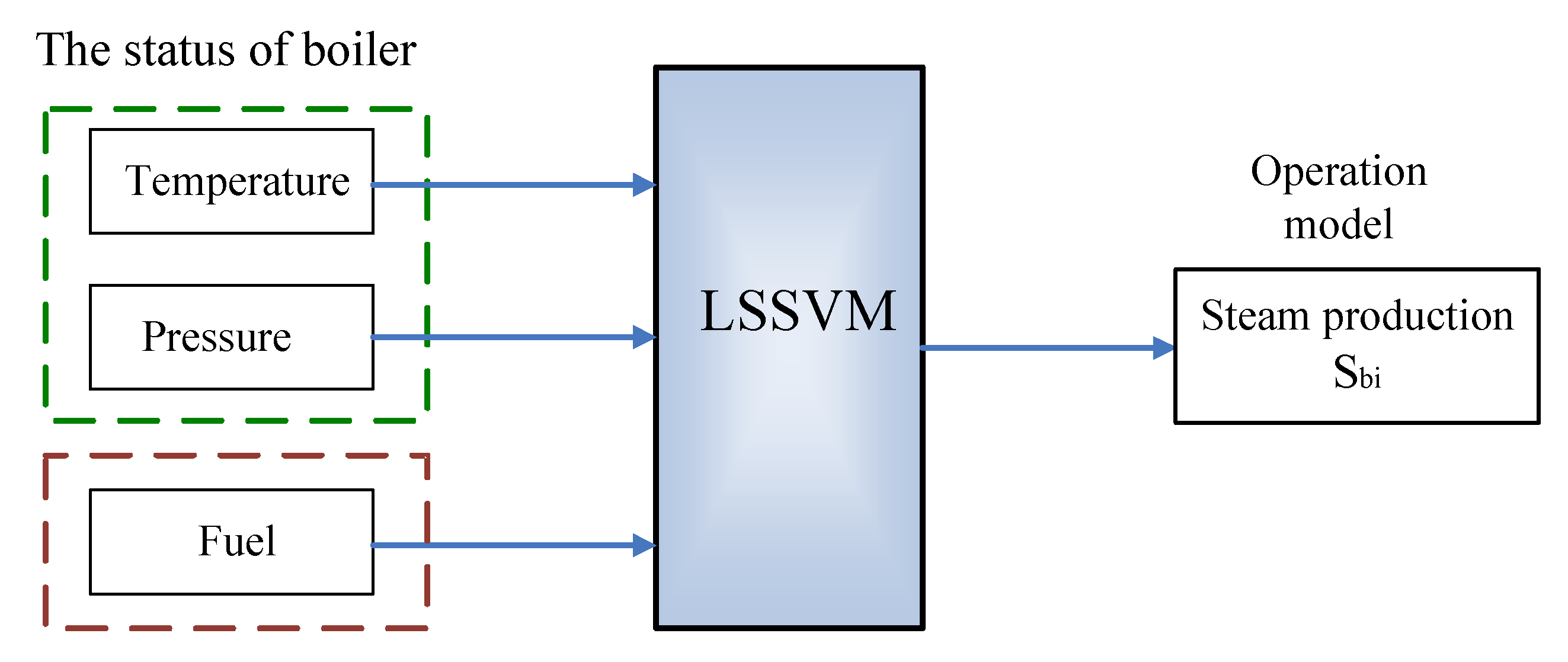
By using the Least-Square Support Vector Machine (LSSVM) [33], the operation models of boilers can be calculated from boiler operational records as shown in Figure 2. The temperature, pressure, fuel consumption, and steam generation for a real cogeneration system are measured from the operational data of boilers. The LSSVM is used for model training, and the input layer data are transferred to the output layer through the LSSVM. In general, using the Radial Basis Function Network (RBFN) kernel function, , can yield a good prediction of the LSSVM model. Therefore, we adopt the RBFN kernel function as the kernel function of the LSSVM model. The error is calculated by using Mean Absolute Percentage Error (MAPE) as shown in Equation (1):
where is actual operation data to be predicted is the operation data constructed with LSSVM, and is total training time.
2.2. Operation Model of Steam Turbines
The steam from back-pressure steam turbines flows to the single inlet. After the high temperature and high pressure steam enters the steam turbine, the pressure reduces, the volume expands, and the temperature reduces. The steam in the outlet end is the 20 kg/300 °C medium pressure steam required for the process. The operation of the back-pressure steam turbine relies on the relationship between steam flow at the outlet and the generated electricity; the operation model of the back-pressure steam turbine is constructed by LSSVM, as shown in Figure 3.
Extraction condensing turbines are different from the backpressure turbines, meaning the extraction condensing turbines have a single steam inlet. In the multi sections, after extraction of the middle/low pressure steam and exhaust of the steam at the final section, the condensing turbines are shown as in Figure 1. LSSVM is used to construct the generated electricity functions between the process steam outlet flow and the steam flow at the condensing section. The operation model constructed by LSSVM is shown in Figure 4.
2.3. Emission Model
emission models may be defined based upon the amount of fuel consumed. The model of emission for is formulated by the IPCC [34] as:
, approximated by the three order function gives the thermal conductivity of each kind of unit. are the coefficients of the emission of unit i. is the carbon emission parameter of unit i (21.1 kg-C/GJ for oil, 25.8 kg-C/GJ for coal, 15.3 kg-C/GJ for natural gas) and is the carbon oxidizing rate of unit i (0.99 for oil, 0.98 for coal, 0.995 for natural gas).
2.4. Objective Function and Constraints
The purpose of the proposed scheme is to maximize profit while satisfying operational constraints. The objective function, including profit from steam sold, profit from electricity sold, fuel costs, emissions costs, wheeling costs, and water costs, is formulated in Equation (3):
(1) The profit from thermal steam sold:
(2) The profit from electricity sold:
(3) The cost of fuel:
(4) Emission costs:
(5) Wheeling costs:
(6) The cost of pure water:
Cc: The charged emission price for CO2.(NT$235/ton) [35]; Fbi(Sbi(t)): consumed enthalpy of the i steam boiler at t hour; Fuel_cost: The fuel cost(NT$/MBTU) for coal, gas, and oil; Sout(t): The thermal steam sold at time t (ton/h); Steamcost: The price of thermal steam sold (NT$/ton); Ptie(t): The electricity sold to utility at time t; TOU(t): Time-of-Use rate (NT$/KWH), as shown in Table 1 [32]; Wb(t): The water used by boilers at time t (ton/h); WC: The cost of water (NT$/ton); WUC: the wheeling cost (NT$/MWH).
The operation constraints are considered as follows:
(1) Power balance in the power system:
(2) Steam balance for boilers, turbines, sold, and industrial processes:
(3) Operation constraints for boilers, steam turbines and power generation:
Dh(t), Dm(t): The high/medium pressure steam demands of industry at time t (T/h); Pload(t): The load of cogeneration system at time t; , : Minimal/maximal limits of steam for boiler i; , : Minimal/maximal limits of high pressure steam for turbine i; , : Minimal/maximal limits of medium pressure extraction steam for turbine i; , : Minimal/maximal limits of medium pressure exhausted steam for turbine i; , : Minimal/maximal limits of the generated power for turbine i.
3. Solution Algorithm
This study proposes an EACO, which combines the ACO and Genetic Algorithm (GA), in order to achieve the optimal energy trading dispatch of a cogeneration system. Crossover and mutation mechanisms are integrated into the ACO procedure, and serve to generate offspring in order to escape from the local optimum. The EACO procedure applied in the energy trading dispatch of a cogeneration system is described as follows.
(1) Input Data
Input data includes high/medium steam demand, internal load, plant type, plant capacity, and number of plants.
(2) Set EACO Parameters
EACO parameters include the population of ants (k), the number of generations (G), initial pheromone (), the relative influence of the pheromone trail (), the relative influence of the heuristic information (), and the pheromone evaporation rate ().
(3) Initialized Individuals
is an individual, i = 1, 2, …, k. k, which is the number of ants, is set to 30 in our study. s is the number of parameters. All individuals are set between the minimal and maximal limits with a uniform distribution as shown in Equation (19). The fitness score of each is obtained by calculating the objective function () by considering Equations (10)~(18). The fitness values were arranged in descending order from the maximum () to the minimum ().
Rand: The uniform random number in (0,1).
(4) The State Transition Rule
The state-based ants are generated according to the level of pheromone and constrained conditions. The transition probability for the from one state s to the next j is at the interval, as given in Equation (20):
where and are the inverse of the edge distance at the generation, which are defined as Equations (21) and (22):
is the objective function as given in Equation (3). and are the score of the and individuals at the interval, and is the optimal fitness score at the interval. is the number of feasible individuals at the interval.
and are the pheromone intensity on edge (s, j) and edge (s, l) at the generation. Ant k positioned on state s chooses to move to the next state by taking account of and ηt,sl. When the value of τt,sl increases, this indicates there has been a lot of traffic on this path and it is therefore more desirable in order to reach the optimal solution. When the value of increases, it indicates that the current state should have a higher probability. Each stage contains several states, while the order of states selected at each stage can be combined as an achievable path deemed to be a feasible solution to the problem.
(5) Ant Reproduction
New ants are generated by the scheme of crossover and mutation. Crossover is a structured recombination operation that exchanges two individual ants. Mutation is the occasional random alteration of an individual. The crossover and mutation scheme is described as follows:
- (i)
- Randomly select two parents, and generate offspring by assigning a Control Variable ()
- (a)
- If : Mutation is used;
- (b)
- If : Crossover is used.Rand: the uniform random in [0, 1]; : the control variable between 0.1 to 0.9. The initial value set to 0.5; g: the current iteration number.
- (ii)
- If comes from crossover used, the control variable will be decreased as shown in Equation (23):where is the regulated parameter. When RP is added in the crossover process, the higher probability for crossover operation will produce the next offspring.CV(g + 1) = CV(g) − RP
- (iii)
- If comes from mutation, the control parameter will be increased as shown in Equation (24):CV(g + 1) = CV(g) + DSimilarly, when RP is added in the mutation process, the higher probability for mutation operation will produce the next offspring.
- (iv)
- If , the control variable needs to hold back. If , we have:otherwise,CV(g + 1) = CV(g) − DCV(g + 1) = CV(g) + D
The crossover operator proceeds to exchange two individual ants by random. and , which are the and individual ants at the interval, are exchanged by the crossover operator. The mutation operation is carried out to produce another individual ant. Each individual ant is mutated and created to a new individual ant by using (27).
represents a Gaussian random variable with mean 0 and variable . can be calculated by:
, which is a mutation factor at the j-th generation, is set within [0, 1].
(6) Update the Pheromone
While building a solution to the problem, the pheromone of a visited route can be dynamically adjusted by Equation (29). This process is called the “local pheromone-updating rule”:
ρ is the constant of pheromone intensity (0 ≤ ρ ≤ 1) and is the deviation of pheromone intensity on edge (s, j) at the t − th interval, as shown in Equation (30):
Q is the release rate of pheromone (0 ≤ Q ≤ 1) and is the path error (s, j) for the k − th ant.
(7) Stopping Rule
If a pre-specified stopping condition is satisfied, the run must be stopped and the results outputted; otherwise, return to step 4. In this study, the stopping rule is set at 300 generations.
4. Case Study
The proposed algorithm was tested with three back-pressure steam turbines, four extraction condenser steam turbines and seven steam boilers using gas, oil, and coal as fuel. Steam generation was measured in the field. All facilities including generators, boilers, and steam turbines have their capacity limitation. The limits of all facilities are introduced in Table 2 and Table 3.
4.1. Modeling Tests for Boilers and Steam Turbines
In this paper, the operation data of the boilers in the cogeneration system are recorded during the periods of each normal working day. The number of operation data samples for each boiler is 60; these are used to establish the operational models of boilers 1–7. The error results are shown in Table 4, and the example for operation models of boilers 1–2 are shown in Figure 5.
In this paper, the operation data of the backpressure steam turbines (ST1~3) and extraction condensing steam turbines (ST4~7) in the cogeneration system are recorded and used by LS and LSSVM to establish the operation models of the steam turbines (ST1~7). The error results are shown in Table 5, and the example for the operation curves of steam turbines ST1 and ST6 are shown in Figure 6. The error results for the operation model of steam turbines is from 1.3916% to 2.1475%. It can be proved that the accuracy is reliable.
4.2. Results at Different TOU Intervals
EACO was used to solve the energy dispatch of the cogeneration systems under a liberalized market. In the study system, the internal load was 30 MW and the steam demands of the industry for high- and medium-pressure were 60 T/H and 600 T/H, respectively. Table 6 shows the simulation results at the different TOU intervals. Table 6 indicates that all constraints were met. Since the electricity price is higher at the peak period, the operation strategy of cogeneration systems sold more power to the utility in order to achieve greater benefit. During off-peak periods, the cogeneration systems sell more thermal steam power to attain further benefits. It can be shown that the operation dispatch of the cogeneration systems during the peak period generated 273.321 MW and sold about 243.321 MW to the utility. During the peak period, all generators produced their highest outputs, while tending to sell the thermal steam to industries during semi-peak and off-peak periods. The TOU rate plays an important role in the economic dispatch of a cogeneration system.
Table 7 gives a profit analysis of cogeneration systems at different TOU intervals. The profits during peak period, semi-peak period, and off-peak peroid are 267,678.05, 13,606.32, and −121,047.33, respectively. The profit is lost during the off-peak period. As the cogeneration systems sell more power to utilities during the peak period, greater profits are realized. In the off-peak period, cogeneration systems sell more thermal steam to industries, thereby optimizing the energy trading dispatch. From Table 7, it is noted that the TOU rate influences the profits of the cogeneration system.
4.3. Convergence Test
Table 8 shows the comparisons of EP, GA, PSO, ACO, and EACO during different periods. An IBM PC with a P-IV2.0 GHz CPU and 512 MB SDRAM was used for this test. From this, the improvement of the EACO over other algorithms is clear. Figure 7 shows the convergent characteristics of EP, GA, PSO, ACO, and EACO during the peak period. The average execution times for EACO and ACO were only 1.85 s and 1.67 s, respectively. Although the executed performance of EACO was subtle, it showed the capacity of EACO to explore a solution more likely to offer maximum benefit.
4.4. Robustness Test
Four algorithms including EP, GA, PSO, and ACO, were also tested at the peak period; the results are shown in Table 9. Each algorithm was executed using 100 trials during the robustness test. The number of optimum and average converged profit for EACO are 87 and NT$261,618.29. It is seen that EACO offers a greater ability to attain maximum profits and a higher probability of finding the best solution.
4.5. The Influence of Carbon Price
Table 10 shows the impact of various carbon prices experienced during the peak period. Table 10 suggests that if carbon prices are higher, CO2 emissions will decrease. Similarly, due to the fuel type for extraction-condenser turbines being oil or coal, power generation will be reduced depending upon the carbon price. The purpose of various carbon prices here is to illustrate the tradoff between profit and emission costs, and also to show that generators may more economically dispatch trade electricity or CO2 emission to find better profit.
Figure 8 shows the profit-emission tradeoff curves during the peak period. Figure 8 provides diversified alternatives for decision makers, showing the effects of various carbon prices. Replaced with the maximal allowable emission as a constraint, an appropriate decision can be chosen to satisfy the desired level of profit and emission costs.
5. Conclusions
In this paper, an EACO is proposed to maximize the profit of energy trading using a cogeneration system. The objective function is formulated based upon a maximal profit model, which includes profit from steam sold, profit from electricity sold, fuel costs, CO2 emission costs, wheeling costs, and water costs. By considering the various carbon prices, the profits of the energy trading dispatches are evaluated while considering three different TOU scenarios. The effectiveness of the EACO is demonstrated and simulated on a real cogeneration system. Our analysis points to expectations of the TOU rate or carbon price for the energy trading dispatch. With the advantages of both heuristic ideals and ACO, EACO has threefold conventional ideals: the complicated problem is solvable, with a better performance than ACO, and the more likelihood to get a global optimum than heuristic methods. The results indicate that both provide good tools for determining the optimum energy trading operation of a cogeneration system. This shows that the tradeoff between investment cost and environmental protection can be clearly predetermined in the liberty market. EACO also has great potential to be further applied to many ill-conditioned problems in power system planning and operations.
Author Contributions
W.-M.L. generalized the novel algorithms and designed the system planning projects. C.-Y.Y. used system parameters and models for the simulation test. M.-T.T. performed the editing and experimental model results. H.-S.H. written the orginal draft perparation. C.-S.T. provided hardware tools and system model related materials. All the authors were involved in exploring system validation and results, and permitting the benefits of the published document.
Funding
This research was funded by Ministry of Science and Technology of R.O.C. grant number MOST 107-2221-E-230-008-MY3.
Conflicts of Interest
The authors declare no conflict of interest.
References
- Aluisio, B.; Dicorato, M.; Forte, G.; Trovato, M. An optimization procedure for Microgrid day-ahead operation in the presence of CHP facilities. Sustain. Energy Grids Netw. 2017, 11, 34–45. [Google Scholar] [CrossRef]
- Motevasel, M.; Seifi, A.R.; Niknam, T. Multi-objective energy management of CHP (combined heat and power)-based micro-grid. Energy 2013, 51, 123–136. [Google Scholar] [CrossRef]
- Basu, A.K.; Bhattacharya, A.; Chowdhury, S.; Chowdhury, S.P. Planned Scheduling for Economic Power Sharing in a CHP-Based Micro-Grid. IEEE Trans. Power Syst. 2012, 27, 30–38. [Google Scholar] [CrossRef]
- Isa, N.M.; Tan, C.W.; Yatim, A. A comprehensive review of cogeneration system in a microgrid: A perspective from architecture and operating system. Renew. Sustain. Energy Rev. 2018, 81, 2236–2263. [Google Scholar] [CrossRef]
- Farghal, S.; El-Dewieny, R.; Riad, A. Optimum operation of cogeneration plants with energy purchase facilities. IEE Proc. C Gener. Transm. Distrib. 1987, 134, 313–319. [Google Scholar] [CrossRef]
- Rooijers, F.; Van Amerongen, R. Static economic dispatch for co-generation systems. IEEE Trans. Power Syst. 1994, 9, 1392–1398. [Google Scholar] [CrossRef]
- Al Asmar, J.; Lahoud, C.; Brouche, M. Decision-making strategy for cogeneration power systems integration in the Lebanese electricity grid. Energy Procedia 2017, 119, 801–805. [Google Scholar] [CrossRef]
- Skorek-Osikowska, A.; Remiorz, L.; Bartela, Ł.; Kotowicz, J. Potential for the use of micro-cogeneration prosumer systems based on the Stirling engine with an example in the Polish market. Energy 2017, 133, 46–61. [Google Scholar] [CrossRef]
- Asano, H.; Sagai, S.; Imamura, E.; Ito, K.; Yokoyama, R. Impacts of time-of-use rates on the optimal sizing and operation of cogeneration systems. IEEE Trans. Power Syst. 1992, 7, 1444–1450. [Google Scholar] [CrossRef]
- Lee, C.-H.; Huang, S.-C.; Chang, C.-A.; Chen, B.-K. Operation of Steam Turbines under Blade Failures during the Summer Peak Load Periods. Energies 2014, 7, 7415–7433. [Google Scholar] [CrossRef] [Green Version]
- Gambini, M.; Vellini, M.; Stilo, T.; Manno, M.; Bellocchi, S. High-Efficiency Cogeneration Systems: The Case of the Paper Industry in Italy. Energies 2019, 12, 335. [Google Scholar] [CrossRef]
- Jayakumar, N.; Subramanian, S.; Ganesan, S.; Elanchezhian, E. Grey wolf optimization for combined heat and power dispatch with cogeneration systems. Int. J. Electr. Power Energy Syst. 2016, 74, 252–264. [Google Scholar] [CrossRef]
- Nguyen, T.T.; Vo, D.N.; Dinh, B.H. Cuckoo search algorithm for combined heat and power economic dispatch. Int. J. Electr. Power Energy Syst. 2016, 81, 204–214. [Google Scholar] [CrossRef]
- Tsay, M.-T.; Lin, W.-M.; Lee, J.-L. Application of evolutionary programming for economic dispatch of cogeneration systems under emission constraints. Int. J. Electr. Power Energy Syst. 2001, 23, 805–812. [Google Scholar] [CrossRef]
- Tsay, M.-T.; Lin, W.-M.; Lee, J.-L. Interactive best-compromise approach for operation dispatch of cogeneration systems. IEE Proc. Gener. Transm. Distrib. 2001, 148, 326. [Google Scholar] [CrossRef]
- Carpaneto, E.; Chicco, G.; Mancarella, P.; Russo, A. Cogeneration planning under uncertainty: Part I: Multiple time frame approach. Appl. Energy 2011, 88, 1059–1067. [Google Scholar] [CrossRef]
- Thorin, E.; Brand, H.; Weber, C. Long-term optimization of cogeneration systems in a competitive market environment. Appl. Energy 2005, 81, 152–169. [Google Scholar] [CrossRef]
- Chen, S.-L.; Tsay, M.-T.; Gow, H.-J. Scheduling of cogeneration plants considering electricity wheeling using enhanced immune algorithm. Int. J. Electr. Power Energy Syst. 2005, 27, 31–38. [Google Scholar] [CrossRef]
- Yusta, J.; Jesus, P.D.O.-D.; Khodr, H.; Jesus, P.D.O.-D. Optimal energy exchange of an industrial cogeneration in a day-ahead electricity market. Electr. Power Syst. Res. 2008, 78, 1764–1772. [Google Scholar] [CrossRef]
- Safder, U.; Ifaei, P.; Yoo, C. Multi-objective optimization and flexibility analysis of a cogeneration system using thermorisk and thermoeconomic analyses. Energy Convers. Manag. 2018, 166, 602–636. [Google Scholar] [CrossRef]
- He, L.; Lu, Z.; Pan, L.; Zhao, H.; Li, X.; Zhang, J. Optimal Economic and Emission Dispatch of a Microgrid with a Combined Heat and Power System. Energies 2019, 12, 604. [Google Scholar] [CrossRef]
- Chang, H.-H. Genetic algorithms and non-intrusive energy management system based economic dispatch for cogeneration units. Energy 2011, 36, 181–190. [Google Scholar] [CrossRef]
- Basu, M. Artificial immune system for combined heat and power economic dispatch. Int. J. Electr. Power Energy Syst. 2012, 43, 1–5. [Google Scholar] [CrossRef]
- Gambardella, L.; Dorigo, M. Ant colony system: A cooperative learning approach to the traveling salesman problem. IEEE Trans. Evol. Comput. 1997, 1, 53–66. [Google Scholar]
- Mullen, R.J.; Monekosso, D.; Barman, S.; Remagnino, P. A review of ant algorithms. Expert Syst. Appl. 2009, 36, 9608–9617. [Google Scholar] [CrossRef]
- Saravuth, P.; Issarachai, N.; Waree, K. Ant colony optimisation for economic dispatch problem with non-smooth cost functions. Int. J. Electr. Power Energy Syst. 2010, 32, 478–487. [Google Scholar]
- Priyadarshi, N.; Ramachandaramurthy, V.K.; Padmanaban, S.; Azam, F. An Ant Colony Optimized MPPT for Standalone Hybrid PV-Wind Power System with Single Cuk Converter. Energies 2019, 12, 167. [Google Scholar] [CrossRef]
- Church, C.; Morsi, W.; El-Hawary, M.; Diduch, C.; Chang, L. Voltage collapse detection using Ant Colony Optimization for smart grid applications. Electr. Power Syst. Res. 2011, 81, 1723–1730. [Google Scholar] [CrossRef]
- Zhou, J.; Wang, C.; Li, Y.; Wang, P.; Li, C.; Lu, P.; Mo, L. A multi-objective multi-population ant colony optimization for economic emission dispatch considering power system security. Appl. Math. Model. 2017, 45, 684–704. [Google Scholar] [CrossRef]
- Kıran, M.S.; Özceylan, E.; Gunduz, M.; Paksoy, T. A novel hybrid approach based on Particle Swarm Optimization and Ant Colony Algorithm to forecast energy demand of Turkey. Energy Convers. Manag. 2012, 53, 75–83. [Google Scholar] [CrossRef]
- Goldberg, D.E. Genetic Algorithm in Search, Optimization and Machine Learning; Addison Wesley: Boston, MA, USA, 1989. [Google Scholar]
- Taiwan Power Company (TPC). Time-of-Use Rate for Cogeneration Plants. The electricity Rates Structure for Taipower Company; Taiwan Power Company (TPC): Taipei, Taiwan, 2017. [Google Scholar]
- Suykens, J.A.K.; Vandewalle, J. Least square support vector machine. Neural Process. Lett. 1999, 9, 293–300. [Google Scholar] [CrossRef]
- Intergovernmental Penal on Climate Change. Available online: http://www.ipcc.com/ (accessed on 8 April 2017).
- Nord Pool Power Exchanger. Available online: http://www.nasdaqomx.com/commodities (accessed on 11 April 2017).
Figure 1.
Energy flow of a cogeneration system.

Figure 2.
Operation model of boilers using the LSSVM.

Figure 3.
Operation model of the back-pressure steam turbine using the LSSVM.

Figure 4.
Operation model of the extraction condensing steam turbines using LSSVM.

Figure 5.
Example of the operation models of boilers 1–2.

Figure 6.
Example for the operation models of steam turbines (ST1/ST6).

Figure 7.
Convergence characteristics of EP, GA, PSO, ACO, and EACO during the peak period.

Figure 8.
Profit-emission tradeoff curves during the peak period.


Table 1.
The time-of-use rates of Taipower Company.
| Electricity Sale Rate (NT$/KWH) | Utility Buy-Back Rate NT$/KWH | ||
|---|---|---|---|
| Level 1 | Level 2 | ||
| Peak Period | 3.04 | 2.7480 | 3.04 |
| Semi-peak Period | 1.83 | 1.5767 | 1.83 |
| Off-peak Period | 0.69 | 0.4729 | 0.69 |
Level 1: power exported at under 20% rated capacity; Level 2: power exported at over 20% rated capacity.
Table 2.
Maximal and minimal limits of boiler flows and generators.
| Unit No. | Fuel Type | Min. (ton) | Max. (ton) | Unit No. | Min. (MW) | Max. (MW) |
|---|---|---|---|---|---|---|
| Boiler1 | Gas | 68 | 137.5 | Gen1 | 4.1 | 10 |
| Boiler2 | Gas | 52 | 120 | Gen2 | 4.9 | 10 |
| Boiler3 | Gas | 60 | 137.5 | Gen3 | 4.4 | 10 |
| Boiler4 | Oil | 52 | 100 | Gen4 | 15.6 | 50 |
| Boiler5 | Coal | 127 | 250 | Gen5 | 20 | 100 |
| Boiler6 | Coal | 84 | 280 | Gen6 | 20 | 100 |
| Boiler7 | Coal | 90 | 300 | Gen7 | 20 | 100 |
Table 3.
Steam output limits.
| Unit No. | Unit Type | Min. (ton/h) | Max. (ton/h) |
|---|---|---|---|
| Mm1 | Back-pressure | 75 | 120 |
| Mm2 | Back-pressure | 55 | 140 |
| Mm3 | Back-pressure | 50 | 80 |
| Mm4 | Extraction condenser steam | 30 | 150 |
| Mm5 | Extraction condenser steam | 30 | 150 |
| Mm6 | Extraction condenser steam | 30 | 150 |
| Mm7 | Extraction condenser steam | 30 | 150 |
| Mw4 | Extraction condenser steam | 20 | 200 |
| Mw5 | Extraction condenser steam | 25 | 300 |
| Mw6 | Extraction condenser steam | 25 | 300 |
| Mw7 | Extraction condenser steam | 25 | 300 |
Table 4.
The error results for the operation model of boilers.
| Unit No. | Number. of Operation Data | LS Error (%) | LSSVM Error (%) |
|---|---|---|---|
| Boiler1 | 60 | 4.0999 | 3.1537 |
| Boiler2 | 60 | 3.0520 | 2.0379 |
| Boiler3 | 60 | 3.1001 | 1.6948 |
| Boiler4 | 60 | 2.9621 | 1.8252 |
| Boiler5 | 60 | 2.6386 | 1.7779 |
| Boiler6 | 60 | 2.6326 | 1.7169 |
| Boiler7 | 60 | 2.7150 | 1.5325 |
Table 5.
The error results for the operation model of steam turbines.
| Unit No. | Number. of Operation Data | LS Error (%) | LSSVM Error (%) |
|---|---|---|---|
| ST1 | 54 | 2.2081 | 1.5324 |
| ST2 | 54 | 2.1404 | 1.4494 |
| ST3 | 90 | 2.1960 | 1.7109 |
| ST4 | 90 | 2.2494 | 1.9637 |
| ST5 | 90 | 2.6757 | 2.1475 |
| ST6 | 135 | 2.0326 | 1.5379 |
| ST7 | 135 | 7.4892 | 1.3916 |
Table 6.
Dispatch results at different TOU intervals.
| TOU | Peak Period | Semi-Peak Period | Off-Peak Period |
|---|---|---|---|
| (MW) | 5.322 | 4.100 | 6.235 |
| (MW) | 6.704 | 5.182 | 5.061 |
| (MW) | 5.355 | 6.175 | 6.362 |
| (MW) | 50.000 | 50.000 | 50.000 |
| (MW) | 70.212 | 33.103 | 32.389 |
| (MW) | 49.873 | 33.967 | 21.210 |
| (MW) | 85.856 | 31.445 | 31.445 |
| Total Generation (MW) | 273.321 | 163.972 | 152.703 |
| (MW) | 243.321 | 133.972 | 122.703 |
| (ton/h) | 521.944 | 129.219 | 98.716 |
| (ton/h) | 0.000 | 535.781 | 566.284 |
Table 7.
Profit analysis of cogeneration systems at different TOU intervals. Unit: NT$/H.
| TOU Item | Peak Period | Semi-Peak Period | Off-Peak Period |
|---|---|---|---|
| The profit for thermal steam sold | 0.00 | 364,331.01 | 385,073.34 |
| The profit from electricity sold | 690,837.19 | 230,485.22 | 74,525.76 |
| The cost of fuel | 350,910.68 | 512,287.60 | 512,287.60 |
| Emissions cost | 199,499.69 | 208,611.45 | 208,611.45 |
| Wheeling cost | 12,166.03 | 6698.62 | 6135.14 |
| The cost for pure water | 13,200.00 | 13,200.00 | 13,200.00 |
| Profit | 267,678.05 | 13,606.32 | −121,047.33 |
Table 8.
Comparison of EP, GA, PSO, ACO, and EACO algorithms. Unit: NT$/H.
| Algorithm | Peak Period | Semi-Peak Period | Off-Peak Period |
|---|---|---|---|
| EP | 263,849.60 | 12,813.87 | −123,289.77 |
| GA | 265,247.33 | 13,104.46 | −122,999.72 |
| PSO | 266,904.29 | 13,489.53 | −122,030.83 |
| ACO | 266,151.07 | 13,104.46 | −122,192.54 |
| EACO | 267,678.05 | 13,606.32 | −121,047.33 |
Table 9.
Robustness test for EP, GA, PSO, ACO, and EACO algorithms in a peak period.
| Algorithm | Maximal Converged Profit (NT$) | Minimal Converged Profit (NT$) | Average Converged Profit (NT$) | Average Number of Generations to Converge | No. of Trials Reaching Optimum | Average Execution Time (s) |
|---|---|---|---|---|---|---|
| EP | 263,849.60 | 243,046.09 | 257,971.45 | 196 | 48 | 1.5341 |
| GA | 265,247.33 | 245,041.34 | 260,068.28 | 237 | 54 | 2.2153 |
| PSO | 266,904.29 | 254,865.39 | 262,555.59 | 173 | 57 | 1.6124 |
| ACO | 266,151.07 | 252,420.70 | 261,618.29 | 213 | 66 | 1.6741 |
| EACO | 267,678.05 | 259,030.88 | 264,500.37 | 184 | 87 | 1.8476 |
Table 10.
The impact of various carbon prices during the peak period.
| Carbon Price (NT$) | Back-Pressure Turbine Generation (MW) | Extraction-Condenser Turbine Generation (MW) | Profit (NT$) | Emission Cost (NT$) |
|---|---|---|---|---|
| 0 | 18.12 | 254.55 | 322,925.81 | 0.00 |
| 400 | 18.00 | 249.85 | 241,469.31 | 74,714.14 |
| 800 | 18.11 | 212.03 | 188,316.27 | 96,104.88 |
| 1200 | 17.52 | 172.72 | 142,085.10 | 99,394.94 |
| 1600 | 17.01 | 154.71 | 111,351.34 | 100,419.06 |
| 2000 | 15.36 | 149.44 | 94,250.70 | 105,522.53 |
| 2400 | 18.17 | 135.76 | 74,312.66 | 108,103.17 |
| 2800 | 18.11 | 135.76 | 56,215.64 | 123,906.39 |
| 3200 | 15.36 | 138.73 | 39,297.50 | 138,744.85 |
© 2019 by the authors. Licensee MDPI, Basel, Switzerland. This article is an open access article distributed under the terms and conditions of the Creative Commons Attribution (CC BY) license (http://creativecommons.org/licenses/by/4.0/).
Share and Cite
MDPI and ACS Style
Lin, W.-M.; Yang, C.-Y.; Tu, C.-S.; Huang, H.-S.; Tsai, M.-T. The Optimal Energy Dispatch of Cogeneration Systems in a Liberty Market. Energies 2019, 12, 2868. https://doi.org/10.3390/en12152868
AMA Style
Lin W-M, Yang C-Y, Tu C-S, Huang H-S, Tsai M-T. The Optimal Energy Dispatch of Cogeneration Systems in a Liberty Market. Energies. 2019; 12(15):2868. https://doi.org/10.3390/en12152868
Chicago/Turabian StyleLin, Whei-Min, Chung-Yuen Yang, Chia-Sheng Tu, Hsi-Shan Huang, and Ming-Tang Tsai. 2019. "The Optimal Energy Dispatch of Cogeneration Systems in a Liberty Market" Energies 12, no. 15: 2868. https://doi.org/10.3390/en12152868
Note that from the first issue of 2016, this journal uses article numbers instead of page numbers. See further details here.