Thermal Effect of Different Laying Modes on Cross-Linked Polyethylene (XLPE) Insulation and a New Estimation on Cable Ampacity

Abstract

This paper verifies the fluctuation on thermal parameters and ampacity of the high-voltage cross-linked polyethylene (XLPE) cables with different insulation conditions and describes the results of a thermal aging experiment on the XLPE insulation with different operating years in different laying modes guided by Comsol Multiphysics modeling software. The thermal parameters of the cables applied on the models are detected by thermal parameter detection control platform and differential scanning calorimetry (DSC) measurement to assure the effectivity of the simulation. Several diagnostic measurements including Fourier infrared spectroscopy (FTIR), DSC, X-ray diffraction (XRD), and breakdown field strength were conducted on the treated and untreated specimens in order to reveal the changes of properties and the relationship between the thermal effect and the cable ampacity. Moreover, a new estimation on cable ampacity from the perspective on XLPE insulation itself has been proposed in this paper, which is also a possible way to judge the insulation condition of the cable with specific aging degree in specific laying mode for a period of time.

1. Introduction

Thermoplastics are widely used in the insulation of power cables, such as polyvinyl chloride (PVC), low density polyethylene (LDPE), and cross-linked polyethylene (XLPE), which possess higher physical, electrical, and heat-resistant properties compared with oil-paper insulation [1]. The PVC insulation is commonly applied in low-voltage and medium-voltage cables, of which the permissible long-term load temperature is 70 °C [2]; the LDPE power cables can be operated at higher voltage levels by adding special additives [3]. In addition, the permissible long-term load temperature is 75 °C and the permissible maximum short-circuit temperature is 130 °C. Due to the crosslinking treatment of PE, the permissible long-term load temperature and the permissible maximum short-circuit temperature have been elevated to 90 and 250 °C, respectively [4]. The XLPE cables have been widely applied in high-voltage (HV) and extra-high voltage (EHV) transmission systems due to the its high performance on electricity and thermal properties. Therefore, it is meaningful to expand the research frontiers about the XLPE cables in the actual operation to elevate the permissible long-term load capacity and extend their service life.

XLPE is a high-molecular polymer with crystal and amorphous phase, which is subjected mostly to the thermal effect because the crystal structure of XLPE is prone to be affected by the melting and cooling process [5]. It is well evidenced that long-term thermal effect can change the morphology of the insulation distinctly and lead to degradation on the insulation [6,7]. In fact, the influence of thermal effect on polymers is a complicated process and the insulation properties can be improved in some certain situations [8]. Much research has been carried out on this subject. The inverse temperature effect is presented to indicate that the degradation of semi-crystalline polymers is obvious at the low temperatures and a significant recovery at elevated temperatures [9]. In the study about the non-isothermal melt-crystallization kinetics of polymers [10,11], it is well known that the ability of XLPE to crystallize is highly dominated by the cooling rate and the current melting condition of XLPE, because different melting and cooling rates can change the form of spherulites, the size and distribution level of which determine some specific conductive properties of XLPE [12,13]. Therefore, it is meaningful to investigate the changes of properties on XLPE with different melting and cooling rates.

During its practical operation, cable ampacity is influenced by many factors, such as the kind of laying modes and cable specifications [14,15]. Although the factor of the laying mode has been taken into account in International Electrotechnical Commission (IEC) and Institute of Electrical and Electronics Engineers (IEEE) standards in the calculation of cable ampacity, the influence of cable aging on the cable ampacity was rarely concerned. It is universal to calculate the XLPE cable ampacity by the thermal-circuit method and simulation software, which follows the basic rule of calculating the maximum current through the conductor corresponding to the steady-state temperature of 90 °C in different environments [16]. The precondition of the cable ampacity calculation is setting the volumetric thermal capacity and thermal resistance of XLPE as fixed values [17,18,19]. To a large extent, these methods neglect the changes on XLPE insulation itself caused by the different aging factors and the influence of the heating and cooling process to the material during the cable operating condition, which would totally change the morphology of XLPE [20,21,22]. It can be inferred that the thermal resistance and thermal capacity of XLPE in the thermal-circuit model are variable for the reason that the microstructure of XLPE is changing with many factors, such as heat and electricity. Moreover, papers [23,24] have found that the measured values of thermal resistance and thermal capacity of XLPE are different distinctly from the IEC standard. Further, it can be considered that the cable ampacity is a fluctuating value rather than a constant as to the same specification XLPE cable in the same environment with the passage of time. Therefore, it is meaningful to pursue a new way to assess the cable ampacity.

This paper has focused on two aspects of the XLPE insulation in order to reveal the changes on XLPE properties and the relationship between thermal effect and cable ampacity. The first aspect concerns the verification of fluctuation on thermal parameters and ampacity of the cable with different insulation conditions. The second aspect provides a new estimation on cable ampacity from the perspective of the changes of XLPE insulation condition, considering the factors of the different operating years and the different laying modes of the cables. Such correlations between the cable insulation and the cable ampacity should be researched further for a better understanding of the cable ampacity and the aging mechanism of XLPE.

2. Experimental

2.1. Preparation of XLPE Specimens

Two retired high-voltage AC XLPE cables with service years of 15 and 30, and a spare high-voltage AC XLPE cable were selected in this paper. For convenience, they are named by their service year: XLPE-0, XLPE-15, and XLPE-30. Some critical parameters of these cables are listed in

Table 1. Critical parameters of the cables.

Cable	VL	MI	MC	dI	OP
XLPE-0	110/63.5	XLPE	Cu	18.5	1998-
XLPE-15	110/63.5	XLPE	Cu	18.5	1999–2015
XLPE-30	110/63.5	XLPE	Cu	18.5	1985–2015

V_L—voltage level in kV, M_I—insulation material, M_C—conductor material, d_I—insulation thickness in mm, O_P—operation period. Other parameters such as cross-linking method are unknown.

.

Overheated operation has not been reported for these two retired cables, which means that the temperature in the insulation layer remained below 90 °C during the cable operation. Each cable insulation was peeled parallel to the conductor surface, and the tape-like XLPE peels were obtained. Peels near the inner semi-conductive layer were taken as the specimens, because these positions of the insulation endured the most severe electrical and thermal stresses. These obtained specimens were all cleaned by alcohol to remove the surface impurities.

2.2. Cable Thermal Parameters and Ampacity Measurement

By means of the high-voltage cable thermal parameter detection control platform, as illustrated in Figure 1, the three cables with the length of 1.5 m were taken to test its ampacity under the air-laying mode. The critical thermal parameters and ampacity of these three cables are listed in

Table 2. Critical thermal parameters and ampacity of the cables.

Cable	$\mathit{\delta }$ (J/K·m3)	$\mathit{R}$ (K·m/W)	$\mathit{\lambda }$ (W/K·m)	${\mathit{\theta }}_{\mathit{O}}$ (°C)	${\mathit{\theta }}_{\mathit{C}}$ (°C)	${\mathit{I}}_{\mathit{A}}$ (A)
XLPE-0	1.94 $\times$ 106	3.23	0.31	17.7	89.6	1244.07
XLPE-15	1.96 $\times$ 106	3.45	0.29	17.7	89.7	1222.99
XLPE-30	2.07 $\times$ 106	5.26	0.19	17.7	90.2	1096.47

$\delta$—volumetric thermal capacity of cross-linked polyethylene (XLPE), $R$—thermal resistance of XLPE, $\lambda$—thermal conductivity of XLPE, ${\theta }_O$—ambient temperature, ${\theta }_C$—conductor steady-state temperature and $I_A$—ampacity under the air-laying mode.

, where volumetric thermal capacity $\delta$ of XLPE was measured by differential scanning calorimetry (DSC) at the temperature of 30 °C; thermal resistance $R$ of XLPE and thermal conductivity $\lambda$ of XLPE were deducted by thermal circuit model and its Matlab program, and results are shown in the Appendix A; ambient temperature ${\theta }_O$ and conductor steady-state temperature ${\theta }_C$ were measured by thermocouples, and the ampacity under the air-laying mode $I_A$ was tracked by the Matlab program.

From the results in Table 2, it can be verified that the thermal parameters and ampacity fluctuated with different conditions (thermal history, operating years or material characteristic) of the XLPE insulation. Therefore, it is meaningful to provide new estimations on cable ampacity to improve the current research on cable ampacity.

The structural model and thermal parameters in Table 2 of these cables with the same specification is the foundation of the subsequent analysis on simulation of different laying modes based on Comsol Multiphysics. The configuration of the experimental cables is shown in Figure 2.

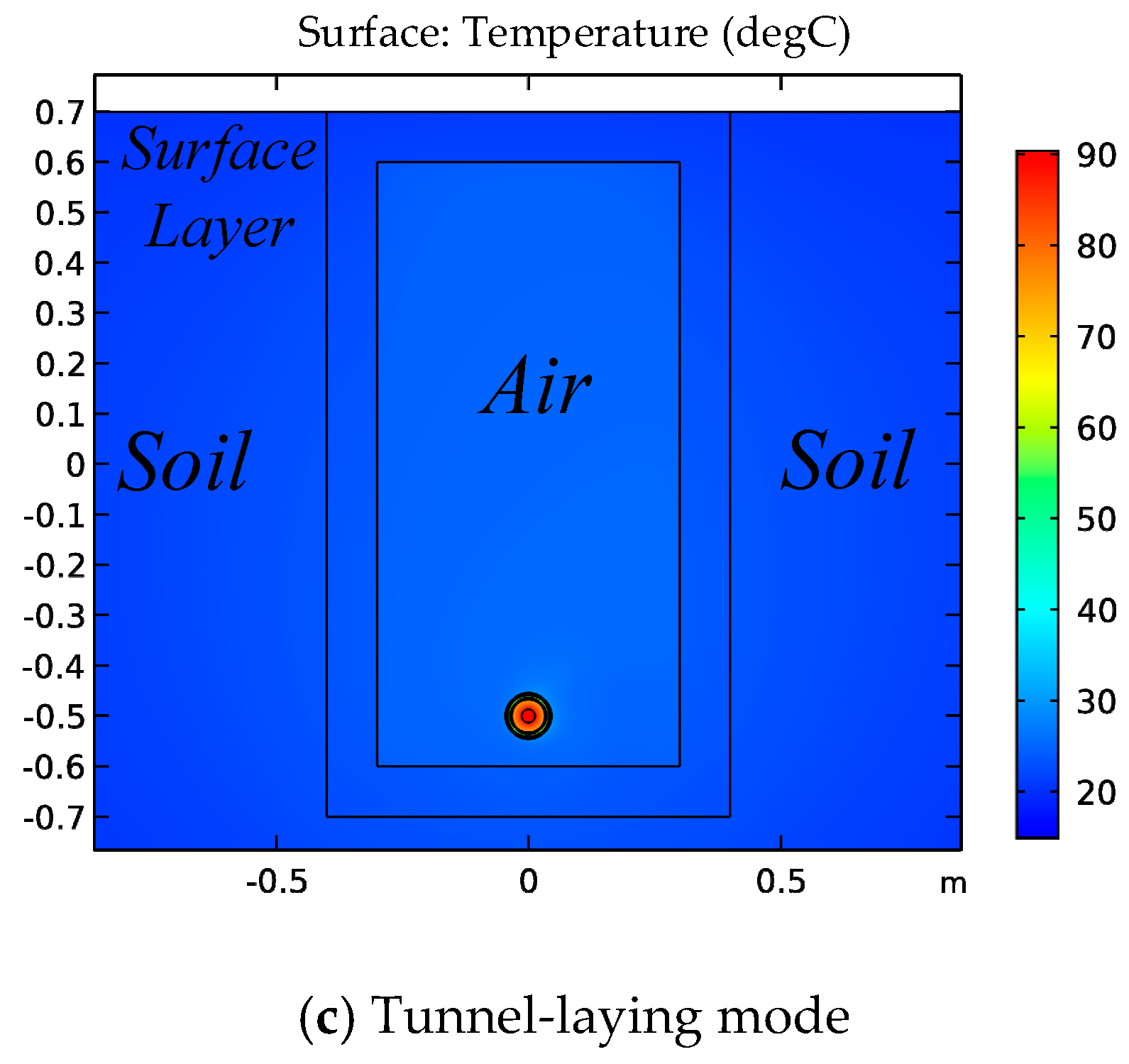
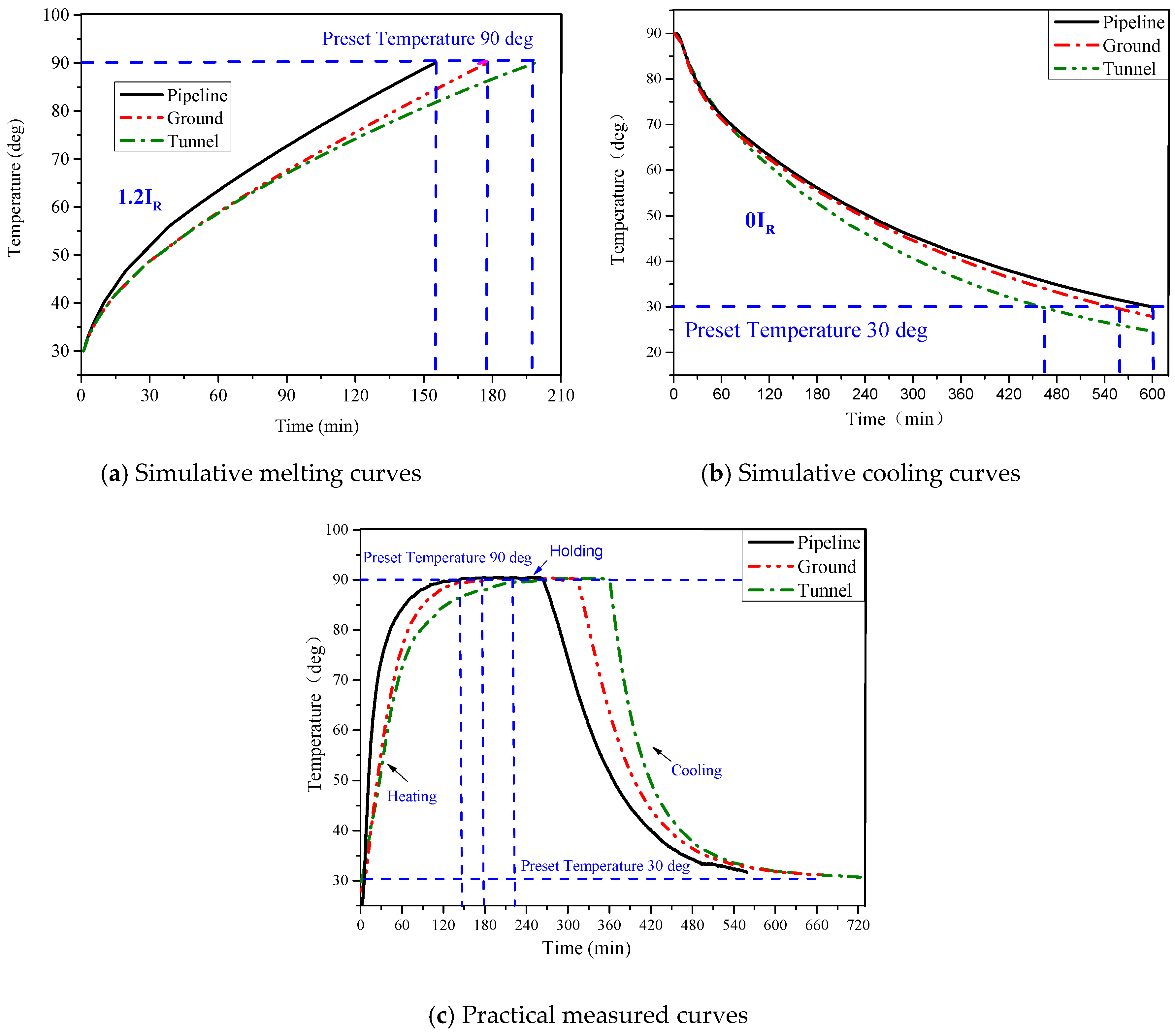
2.3. Simulation of Different Laying Modes of Cables

Comsol Multiphysics was adopted to simulate different laying modes of the XLPE cables. The thermal parameters of the three cables listed in Table 2 were extracted to construct the simulation model, respectively, and we found that the simulation results had the same changing tendency. The permanents of XLPE-0 were used to construct the following simulation model. The establishment of thermal field model and determination of the boundary conditions are not the highlight in this paper, the detail can be referred to literature [25,26,27].

Firstly, we constructed the structural model (Figure 2) under the air-laying mode on the Comsol Multiphysics and we found that the simulative ampacity approached to the practical experiment, which was 1152 A. Therefore, it is assured that the following simulative results are effective.

Secondly, we defined cable ampacity under air-laying mode as reference cable ampacity I_R (I_R = 1200 A) and constructed the structural models into three different laying modes, including pipeline, ground, and tunnel-laying modes based on Comsol Multiphysics, as shown in Figure 3.

Thirdly, we applied the 1.2 I_R and the 0 I_R into the simulated cables, which were laid in pipeline, underground, and in the tunnel, respectively, and obtained the simulative melting and cooling curves of three different laying modes that are shown in Figure 4a,b.

2.4. Thermal Aging

The cable specimens with different operation years were formed into a group, and there were four groups in total. The first group was the untreated group which played a role of reference. The second group simulated the cable laying in the pipeline with the lowest heat dissipation efficiency. The third group simulated the cable laying under the ground with the moderate heat dissipation efficiency. The last group simulated the cable laying in the tunnel with the highest heat dissipation efficiency.

Thermal aging experiments were performed on the last three groups of the specimens. Three modified aging ovens were used to control the heating and cooling process, which fitted the corresponding simulative curves, and a 2 h constant temperature phase of 90 °C between the heating and cooling phases were added to the thermal aging. The three phases, including heating, holding, and cooling, were repeated 80 times in order to enlarge the differences among the specimens. The practical temperature curves of the three different laying modes are shown in Figure 4c, measured by the thermo-couple sensors.

2.5. Diagnostic Measurements

The Fourier transform infrared spectroscopy (FTIR), the differential scanning calorimetry (DSC) measurement, X-ray diffraction (XRD), and the breakdown field strength measurement were adopted to analyze the properties changes on the specimens after the thermal effects.

Micro-structure changes on the specimens were analyzed by the VERTEX 70 infrared spectrometer manufactured by German. Each specimen was tested at 32 scans in the range of 600~3600 cm⁻¹ with a resolution of 0.16 cm⁻¹ and the signal-to-noise ratio of 55,000:1. The obtained spectra were analyzed by OPUS software.

Thermal properties changes on the specimens were analyzed by the DSC NETZSCH-DSC 214 instrument manufactured by German. Five milligram specimens were prepared to test, with the program of two heating phases and a cooling phase under nitrogen atmosphere to avoid thermal degradation. The temperature was increased from 25 to 140 °C at a rate of 10 °C/min and maintained at 140 °C for 5 min, and then cooled to 25 °C. This scanning was repeated twice per measurement, and the first cooling and second heating phases were analyzed in this paper.

Crystal structure changes on the specimens were analyzed by Bruker D8 ADVANCE X-ray diffractometer manufactured by Germany. The experimental interval of Bragg angle was 2θ = 5°–90° by step size of 0.02° with 0.1 s/step scan rate. The obtained data were analyzed by software of DIFFIAC plus XRD Commander.

Electric properties changes of the specimens were analyzed by the ZJC-100 kV voltage breakdown tester manufactured by China. Each specimen was cut into 50 × 50 × 0.5 mm to test, with the voltage rising rate of 1 kV/s under the transformer oil. The valid AC breakdown field strength of each specimen was measured 5 times to obtain the average breakdown field strength.

3. Results and Discussions

In the process of the thermal effects, the features of each laying mode from the heating and cooling curves were observed in the results of Figure 4. Among the three laying modes, the pipeline mode possesses the quick heating and slow cooling features, the ground mode possesses the moderate heating and slow cooling features, and the tunnel mode possesses the slow heating and quick cooling features. These differences led to the different statuses among the specimens with different operating years. In the following parts, we will focus on the connection among the changes of micro-structure, crystal structure, and external electrical property of each specimen in order to reveal the relationship between the thermal effects and the cable ampacity.

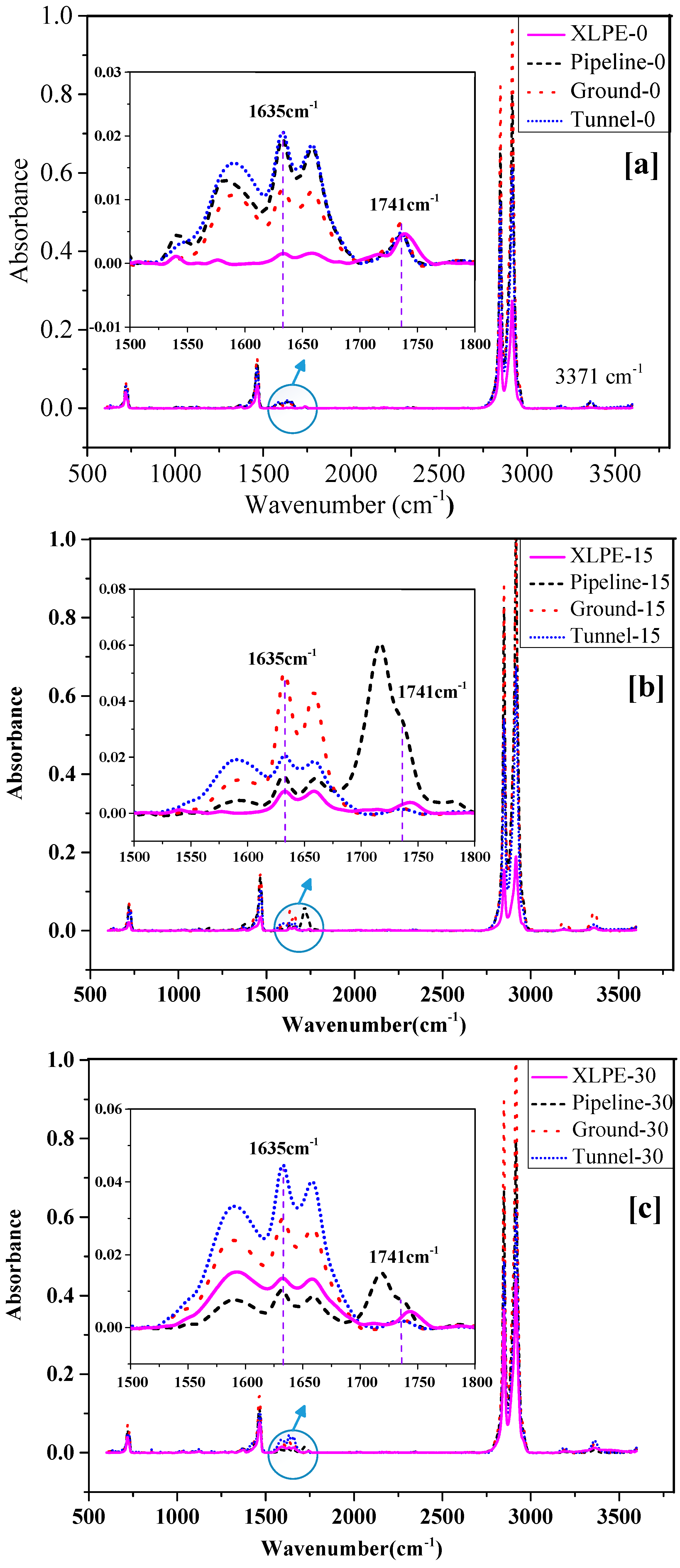
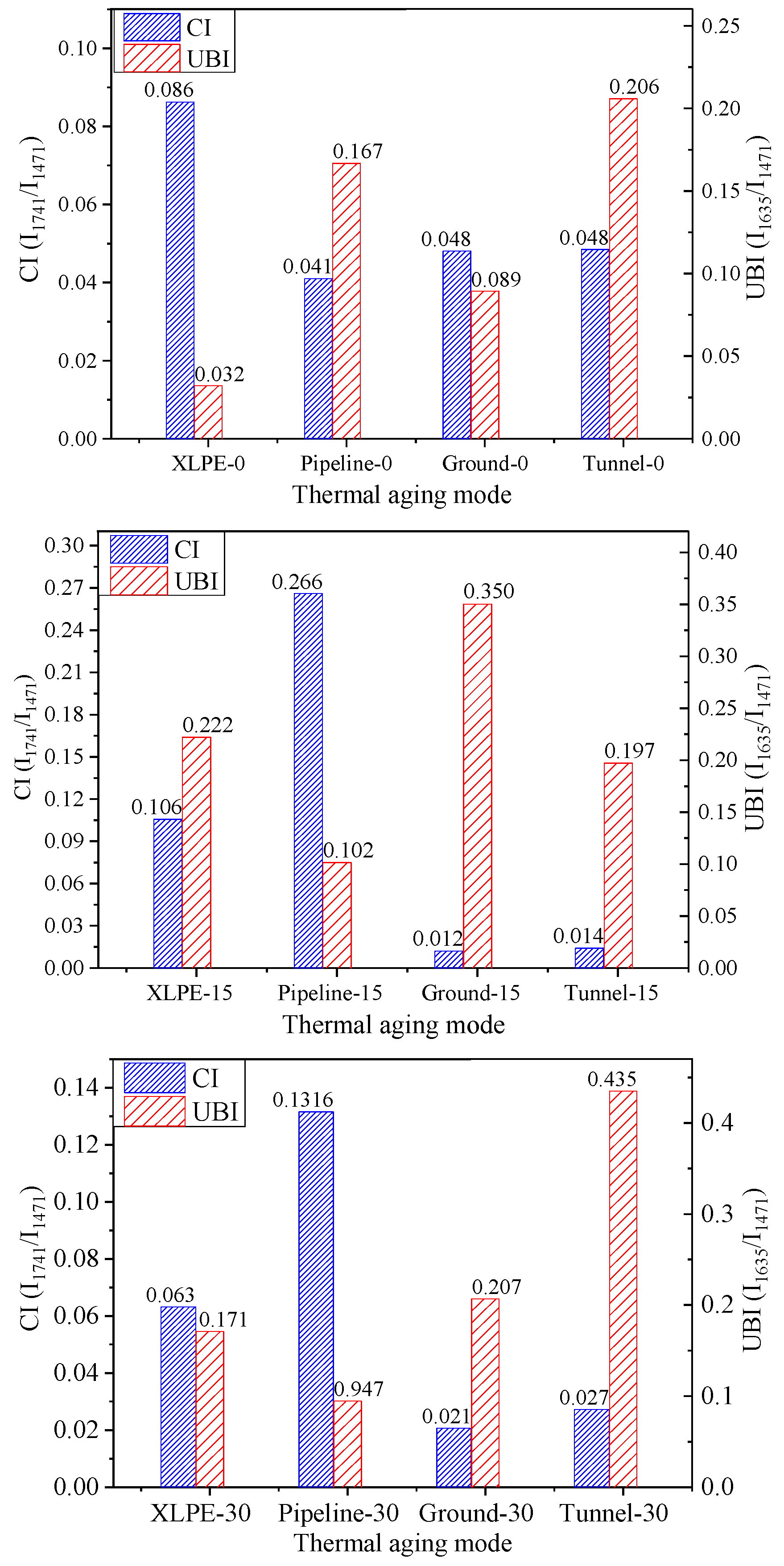
3.1. Result of FTIR Spectroscopy Measurement

The oxidation process of XLPE under the thermal effects can generate major by-products of thermal-oxidation, such as carbonyl groups and unsaturated groups, which can signify the aging status of the specimens. Figure 5 is the FTIR spectra of each specimen whose wavenumber and absorbance represent the kind and content of the corresponding group. The wavelengths of 720, 1471, 2856, and 2937 cm⁻¹ are all caused by the vibration of the methylene band (-CH₂-). Absorption peaks ranging from 1700 cm⁻¹ to 1800 cm⁻¹ can be considered as the thermo-oxidative products [3]. Among of them, carboxylic acid absorption appears at 1701 cm⁻¹, ketone absorption locates at 1718 cm⁻¹, and aldehyde absorption situates at 1741 cm⁻¹. The peak at 1635 cm⁻¹ is assigned to the unsaturated groups absorption, which can indicate the decomposition process.

From Figure 5a, it is clear that some peaks in the range of 1500 to 1700 cm⁻¹ are present after the thermal effects. These peaks reflect a slight decomposition process on the backbone of the XLPE macromolecules. This phenomenon can be associated with the thermal activation to the XLPE molecular chain, which, as a consequence of the adequate motion of the molecular chain, leads to the generation of a certain quantity of small chain segments, free polar groups, etc. On the other aspect, there are no excessive displacement in the position of the peaks in the range of 1700 to 1800 cm⁻¹ among the specimens after thermal aging, which signifies the process of thermo-oxidation is moderate. Therefore, it can be considered that the different thermal aging modes mainly have activated the motion of macromolecular chains, but hardly cause the oxidative degradation in regard to the spare cable.

From Figure 5b, we can see the similar phenomenon happening on the specimens except for Pipeline-15. Significant peaks in the range of 1700 to 1800 cm⁻¹ are presented in Pipeline-15, which is responsible for the aggravation of oxidative degradation. Moreover, there was a pronounced increase in peaks in the range of 1600 to 1650 cm⁻¹ in Ground-15, which indicates a dominant process of chains scission occurs under the thermal effect of ground mode.

From Figure 5c, we can notice that quantities of small molecular chains have emerged on the untreated one (XLPE-30) due to the long-term operation in actual condition. After the thermal aging with different laying modes, it can be deduced that the thermal effects have sped up the decomposition process on the molecular backbone of Ground-0 and Tunnel-0, and a certain quantity of broken molecular chains have already transformed into oxidative groups in Pipeline-30. This indicates severe oxidative degradation occurs in Pipeline-30. It may be admitted that the potential to resist oxidation of XLPE-30 was weakened compared with XLPE-0.

In order to quantify the situation of oxidation and decomposition under the thermal effects, carbonyl index and unsaturated band index were chosen for research. The definition of these two indexes are as follows [3]:

$$CI=\raisebox{1ex}{$I_{1741}$}\!\left/ \!\raisebox{-1ex}{$I_{1471}$}\right.,$$

(1)

$$UBI=\raisebox{1ex}{$I_{1635}$}\!\left/ \!\raisebox{-1ex}{$I_{1471}$}\right.,$$

(2)

where carbonyl index ($CI$) is the relative intensities of the carbonyl band at 1741 cm⁻¹ (aldehyde absorption) to the methylene band at 1471 cm⁻¹; unsaturated band index ($UBI$) is the relative intensities of the unsaturated group at 1635 cm⁻¹ to the methylene band at 1471 cm⁻¹.

The two indexes are shown in Figure 6. It can be stated that the carbonyl index is decreased in all the specimens compared with the untreated ones, except for Pipeline-15 and Pipeline-30, and the unsaturated band index is increased except for Tunnel-15, Pipeline-15, and Pipeline-30. That means the thermal effects aggravate basically the decomposition process of the specimens to generate a certain quantity of broken molecular chains. The oxidation process was followed by chains scission and formation of smaller chain segments, which would easily react with oxygen (O₂) to transform into oxidative groups. For Pipeline-15 and Pipeline-30, the broken molecular chain segments are prone to transform into oxidative groups, probably due to the heating and cooling features of pipeline mode. With regard to Tunnel-15, the two indexes are decreased, which symbolizes the optimization of the micro-structure. As we demonstrated above, the status of the degradation and the stability of the specimens after thermal effects are listed in

Table 3. Status of the degradation and stability of the specimens after thermal effects.

Specimen	Pipeline	Ground	Tunnel
XLPE-0	Improved	Improved	Improved
XLPE-15	Degraded	Maintained	Improved
XLPE-30	Degraded	Improved	Maintained

.

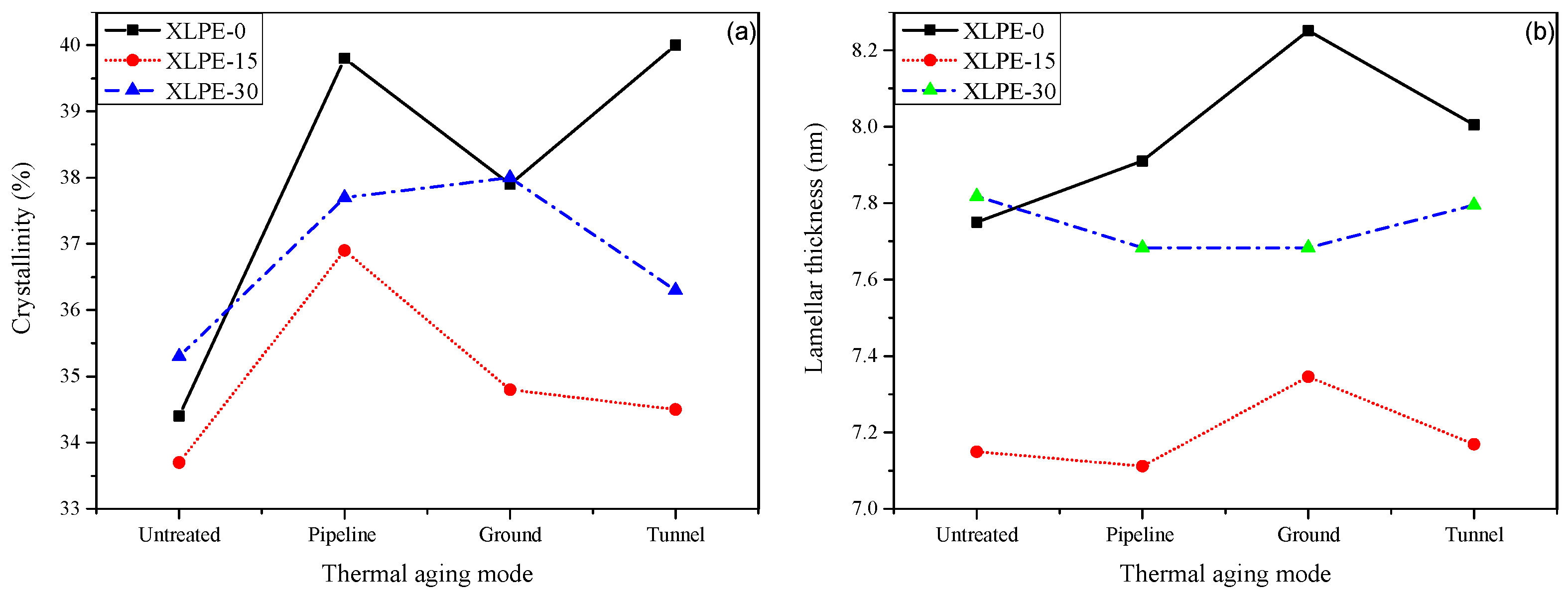
3.2. Result of DSC Measurement

With the program running, two consecutive scans were conducted on each specimen. The first scan began by heating from 30 to 140 °C and then followed by cooling from 140 to 30 °C. The second scan was excerpted in the same way as the first scan. The thermos-gram of the first heating phase is commonly used for observing the thermal history and the current crystalline condition of the specimens, which can also be analyzed by XRD measurement in Section 3.3. In order to avoid long arguments, two phases were analyzed, including the first cooling and the second heating phase, which can be analyzed on the ability to crystallize and the quality of the crystal structure of the specimens after the thermal effects.

Figure 7 and Figure 8 show the thermos-grams of the two phases corresponding to the operating years of each cable. The obtained parameters are listed in

Table 4. Parameters obtained from first cooling and second heating phases.

Specimen	${\mathit{T}}_{\mathit{c}}$ (°C)	$\mathbf{\Delta }{\mathit{H}}_{\mathit{c}}$ (J/g)	${\mathit{T}}_{\mathit{m}}$ (°C)	$\mathbf{\Delta }{\mathit{H}}_{\mathit{f}}$ (J/g)	$\mathbf{\Delta }\mathit{T}$ (°C)
XLPE-0	91.8	−99.0	106.9	100.8	15.1
Pipeline-0	92.0	−108.8	107.6	116.6	15.6
Ground-0	89.7	−102.8	109.0	111.1	19.3
Tunnel-0	90.0	−110.8	108.0	117.2	18.0
XLPE-15	89.0	−93.4	104.0	98.7	15.0
Pipeline-15	88.2	−99.6	103.8	108.1	15.6
Ground-15	86.9	−93.4	105.0	101.9	18.1
Tunnel-15	87.8	−99.1	104.1	101.1	16.3
XLPE-30	89.5	−103.9	107.2	103.4	17.7
Pipeline-30	90.6	−103.0	106.6	110.5	16.0
Ground-30	90.9	−105.1	106.6	111.3	15.7
Tunnel-30	89.8	−104.5	107.1	106.4	17.0

$T_c$—crystallizing peak temperature, $\mathsf{\Delta }{H}_c$—enthalpy of crystallization, $T_m$—melting peak temperature, $\mathsf{\Delta }{H}_f$—enthalpy of fusion and $\mathsf{\Delta }T$—super-cooling degree.

, where $T_c$ is the crystallizing peak temperature, $\mathsf{\Delta }{H}_c$ is the enthalpy of crystallization, $T_m$ is the melting peak temperature, and $\mathsf{\Delta }T$ = $T_m$ − $T_c$ is the degree of supercooling, which is proportional inversely to the crystallization rate [22].

In Figure 7a, it is clearly observed that the exothermic peaks of Ground-0 and Tunnel-0 appear at a slight lower temperature and the shapes become broader, compared to XLPE-0 and Pipeline-0, in the first cooling phase. In Figure 8a, it can be found that melting peaks of all the treated specimens move towards higher temperatures, but the endothermic peaks are expanded. That means that although the thermal effects disperse the crystalline region, especially for Ground-0 and Tunnel-0, the main crystal structure of each treated specimen is improved.

In Figure 7b, exothermic peaks of all the treated specimens displace slightly toward lower temperatures. In Figure 8b, the melting peaks locate at higher temperatures for Ground-15 and Tunnel-15 but at lower temperature for Pipeline-15. The endothermic peaks become broader especially for Pipeline-15. It can be stated that the crystal structure becomes more deteriorated for a long time in the mode of the pipeline.

In Figure 7c or Figure 8c, the exothermic peaks of the treated specimens move towards a higher temperature and the endothermic peaks move towards a lower temperature, which means the thermal effects disrupt the distribution of crystal structure [28]. Therefore, the ability to crystallize is increased, but the quality is declined relatively. Among the specimens, Ground-30 presents the highest crystallization performance.

In addition, the DSC endotherms indicate a range of melting processes that can be related to the crystallinity and lamellar thickness variations. The crystallinity and average lamellar thickness [3,8] can be calculated by Formulas (1) and (2). The calculating formulas are as follows:

$$\chi (\%)=\raisebox{1ex}{$\mathsf{\Delta }{H}_f$}\!\left/ \!\raisebox{-1ex}{$\mathsf{\Delta }{H}_f^0$}\right.\times 100,$$

(3)

$$T_m=T_{m0}\left(1-\raisebox{1ex}{$2{\sigma }_e$}\!\left/ \!\raisebox{-1ex}{$\mathsf{\Delta }{H}_{m}L$}\right.\right),$$

(4)

where $\chi (\%)$ is crystallinity; $\mathsf{\Delta }{H}_f^0$ is the enthalpy of fusion of an ideal polyethylene crystal per unit volume; $T_m$ is the observed melting temperature (K) of lamellar of thickness $L$; $T_{m0}$ is the equilibrium melting temperature of an infinitely thick crystal; ${\sigma }_e$ is the surface-free energy per unit area of basal face; $\mathsf{\Delta }{H}_m$ is the enthalpy of fusion of an ideal polyethylene crystal per unit volume; and $L$ is the lamellar thickness. The used values for calculation were as follows: $T_{m0}$ = 414.6 K, $\mathsf{\Delta }{H}_m$ = 2.88 × 10⁸ J/m³, and ${\sigma }_e$ = 93 × 10⁻³ J/m². Changes on crystallinity and lamellar thickness with different thermal aging modes are depicted in Figure 9.

We can observe that the crystallinity of all the specimens are increased in various degrees after the thermal aging in Figure 9a. This phenomenon is ascribed to adequate movement of the molecular chains and the generation of short chain segments, which are inclined to form the secondary crystal [3]. It is hard to judge the status of crystal structure just from the crystallinity. Therefore, the analysis should be combined with the change of lamellar of thickness obtained at the main endothermic peak shown in Figure 9b. We can find that both Pipeline-15 and Pipeline-30 have a high crystallinity but the lamellar thickness of main endothermic peaks are low, which indicates the crystal structures are mainly made up of secondary crystal. On the contrary, the Ground-0 and the Ground-15 have a relatively low crystallinity with solid lamellar of thickness, which means the crystal structures are firm and compact. Analogously, we can deduce the status of crystal structure of each specimen as shown in

Table 5. Status of the crystal structure of the specimens after thermal effects.

Specimen	Pipeline	Ground	Tunnel
XLPE-0	Improved	Improved	Improved
XLPE-15	Degraded	Improved	Improved
XLPE-30	Degraded	Improved	Maintained

.

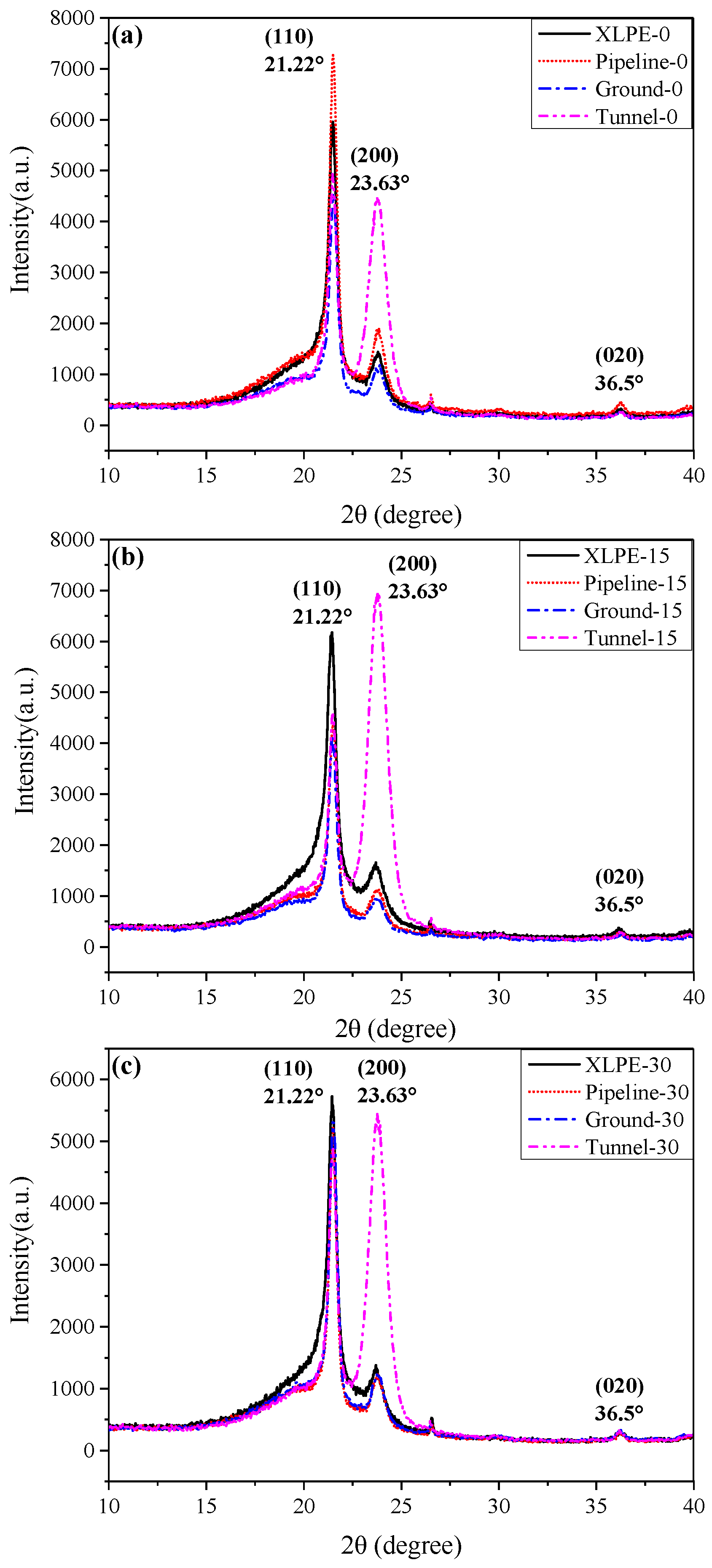
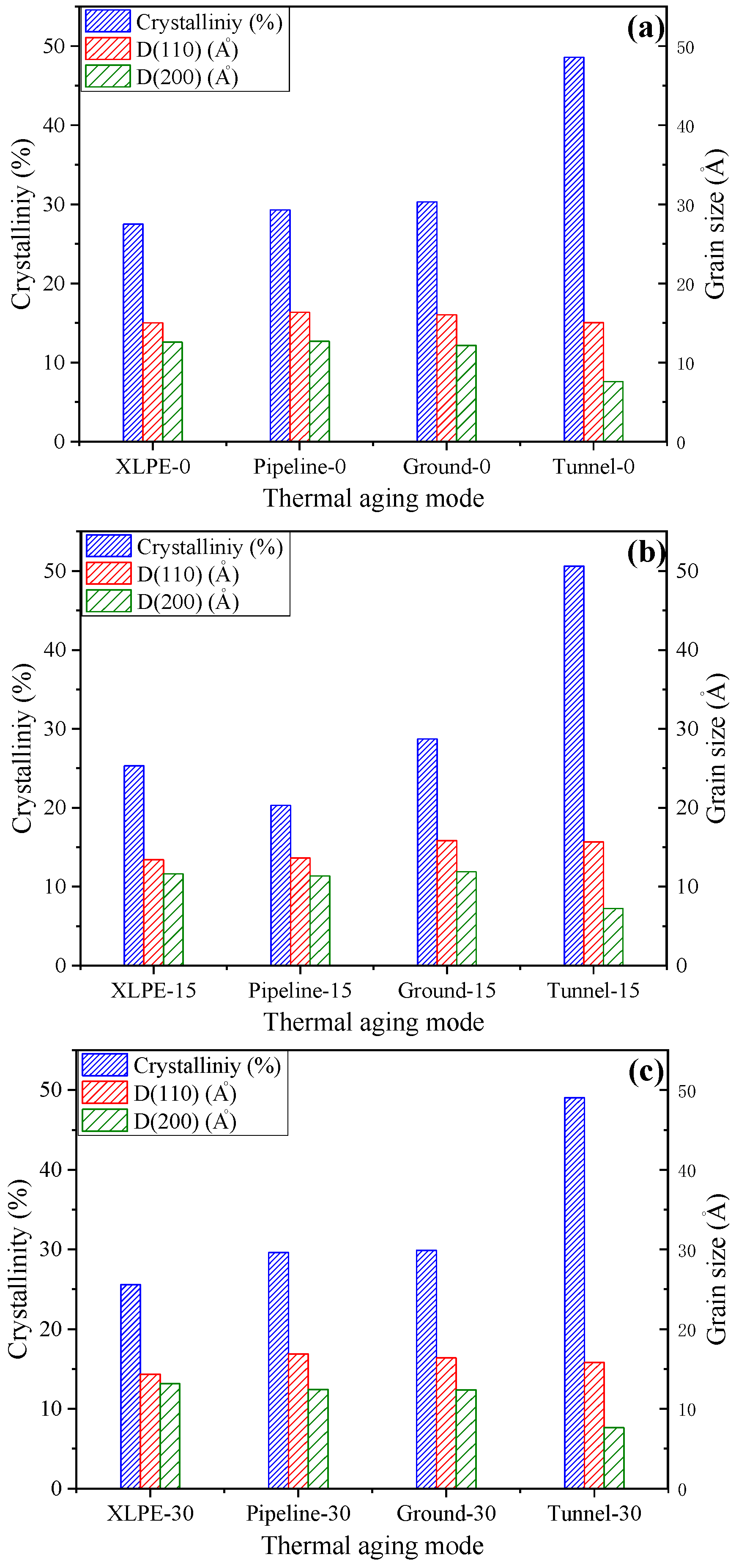
3.3. Result of XRD Measurement

The changes on the crystal structure of each specimen before and after the thermal effect were analyzed by X-ray diffractometer, to observe the influence on the crystalline phase of each layer under the different aging conditions.

Figure 10 displays the X-ray spectrum of each position in cable insulation before and after the accelerated aging test. It can be observed that two main crystalline peaks of each specimen appear at 2θ = 21.22° and 2θ = 23.63°, which correspond to the (110) and (200) lattice planes. There is a one small peak observed at 2θ = 36.5° which corresponds to the (020) lattice plane as Miller demonstrates [29]. There is no excessive displacement in the position of the peaks or in their splitting among the specimens, but the intensity and the shape of the peaks are different. It is indicated that accelerated aging hardly produces any new crystalline phase in the crystal structure, but results in the changes on the crystallinity and the grain size of the specimens.

From Figure 10, it can be noticed remarkably that a turnover phenomenon occurs in the thermal aging of tunnel mode, which is reflected by the fact that the crystal of the (110) lattice plane modifies into the (200) lattice plane. It is commonly assumed that the (200) lattice plane corresponds to the deformed spherulites, whose optical axes are oriented parallel to the radial direction [29]. This transformation indicates the shape of spherulite is associated with the heating and cooling process under different thermal effects. Therefore, we may admit the crystal structure changes on XLPE should be in the light of the features of different laying modes. For more precision on the objective to analyze the crystal structure changes among the specimens, the crystallinity percentage and the grain size are introduced by Formulas (5) and (6).

The crystallinity percentage can be calculated by the Hinrichsen method [30]. The X-ray spectrum of each specimen is fitted by Gaussian functions. Figure 11 displays the corresponding three Gauss fit peaks obtained by using the original 9.1. The calculating process is given as follows:

$$\chi (\%)=\raisebox{1ex}{$(S_2+S_3)$}\!\left/ \!\raisebox{-1ex}{$\left(S_1+S_2+S_3\right)$}\right.\times 100,$$

(5)

where $\chi (\%)$ is crystallinity percentage, $S_1$ is the area of the amorphous halo, $S_2$ is the area of the main crystallization peak at $2\theta$ = 21.22°, and $S_3$ is the area of the secondary crystallization peak at $2\theta$ = 23.63°.

In addition, the grain size of the different diffraction peaks corresponding to different crystal lamellar can be calculated by Scherrer equation [31]. The calculating formula is as follows:

$$D_{hkl}=\raisebox{1ex}{$\left(K·{\lambda }_X\right)$}\!\left/ \!\raisebox{-1ex}{$\left(\beta \cos \theta \right)$}\right.,$$

(6)

where $D_{hkl}$ is the grain size (A) perpendicular to the (hkl) crystal face; ${\lambda }_X$ is experimental X-ray wavelength (nm), which is 0.15418 nm; $\beta$ is the broadening of the diffraction peak (khl) (Rad) producing by grain refinement; and $K$ is 0.89 when $\beta$ is the full width at half maximum of the diffraction peak.

Basing on Formulas (5) and (6), we present the crystallinity percentage and the grain size perpendicular to the (110) and (200) crystal faces in Figure 12. With regard to XLPE-0 in Figure 12a, the crystallinity was lifted up in varying degrees by the disruption of the crystalline order after the thermal effect in each laying mode. Especially for Tunnel-0, a significant increase in crystallinity and distinct shrink in grain size perpendicular to the (200) crystal face indicate that the spherulites are tightly distributed in the insulation and the crystal structure is relatively perfect, even though most of the spherulites were deformed by thermal effect.

With regard to XLPE-15 in Figure 12b, it shows that the changes of the crystallinity and the grain sizes of Ground-15 and Tunnel-15 are similar to the corresponding ones of XLPE-0. The decrease in crystallinity and increase in crystallite size of the principal crystalline area for Pipeline-15 reflect that the spaces among the crystal structures are expanded and the integral crystal structure is not closely arranged.

With regard to XLPE-30 in Figure 12c, minor differences in the crystallinity and the grain sizes between Pipeline-30 and Ground-30 demonstrate that the influence of the features in pipeline and ground modes on the current crystalline condition is not pronounced. For Tunnel-30, we can also find high crystallinity with tight, deformed spherulites, as shown in Figure 12a,b. As we demonstrated above, the status of the current crystal structure of the specimens after thermal effects are listed in

Table 6. Status of the current crystal structure of the specimens after thermal effects.

Specimen	Pipeline	Ground	Tunnel
XLPE-0	Improved	Improved	Improved
XLPE-15	Degraded	Improved	Improved
XLPE-30	Maintained	Maintained	Improved

.

3.4. Results of the Breakdown Field Strength Measurement

The breakdown field strength test was conducted for each specimen and the valid average values are listed in

Table 7. Breakdown field strength (kV/mm).

Specimen	Untreated	Pipeline	Ground	Tunnel
XLPE-0	66.106	69.273	68.860	71.325
XLPE-15	73.489	63.941	75.640	81.650
XLPE-30	68.382	65.463	67.609	69.600

. It is obvious that the electric properties were improved in varying degrees among XLPE-0 specimens after the different thermal effects. This phenomenon is probably attributed to the flexible movement of the molecular chain which activates the development of crystalline order and the annealing effect [6].

With regard to XLPE-15 and XLPE-30, the electric properties were improved under thermal effects in the ground- and tunnel-laying modes, but were degraded in the pipeline-laying mode. It may be considered that the features of the pipeline-laying mode are not relatively suitable for the aged cables with high loading for a long time.

3.5. Assessment of the Structural and Electrical Properties of XLPE under Thermal Effects

From the results of four diagnostic measurements, the correlations between structural and electrical properties were connected to assess the insulation condition.

For the spare cable under the three different thermal effects, the change of temperature activates the adequate movement of the molecular chain, leading to higher crystallinity and electrical performance of the treated specimens. The increase in crystallinity among the specimens is probably ascribed to the scission of the molecules traversing the amorphous regions, followed by rearrangement of the chains imperfectly crystallized at the manufacturing step to increase crystallinity [32]. Moreover, the improvement of crystal structure has a positive influence on the electrical breakdown and the resistivity of the insulation [33].

For the cable with service years of 15, thermal effect in tunnel mode presented a higher performance in structural and electrical properties, which can be identified by the diminution of oxygen-containing groups, improvement of crystalline morphology, and elevation of breakdown field strength. Properties indicators from the diagnostic measurements show a certain degradation happening on thermal effect in pipeline mode with high carbonyl content, inferior crystal structure, and drop in electrical breakdown.

For the cable with service years of 30, the flexibility of the molecular chain and the potential to recrystallize were weakened during long-term practical operation. Thermal effect in pipeline mode reflects degradation from the aspects of carbonyl content, crystal structure, and breakdown field strength compared with XLPE-30. A slight improvement of properties occurs on thermal effect in ground mode and maintaining of properties occurs on thermal effect in tunnel mode.

In this case, compared with the untreated ones, the status of the specimens under different thermal effects can be assessed comprehensively in

Table 8. Comprehensive assessment on the specimens under the thermal effects.

Specimen	Pipeline	Ground	Tunnel
XLPE-0	Improved (greatly)	Improved (greatly)	Improved (greatly)
XLPE-15	Degraded (severely)	Maintained	Improved (greatly)
XLPE-30	Degraded (slightly)	Improved (slightly)	Maintained

.

3.6. A Proposal of New Estimation on Cable Ampacity

With the combination of the reference cable ampacity I_R and the results of diagnostic measurements, the relationship between the cable ampacity and the insulation properties was revealed according to the connection among the change of micro-structure, crystal structure, and external electrical property of each specimen. A new estimation on cable ampacity can be proposed from the perspective of changes of XLPE insulation properties to prolong the cables’ service life. The specific regulation strategy of cable ampacity is as follows:

From the results of Table 8, the improvement and maintenance of overall insulation properties indicate that the margin of reference cable ampacity I_R can be lifted properly to 1.2 I_R. Analogously, the degradation of overall insulation properties indicates that the reference cable ampacity I_R should not be lifted to 1.2 I_R or should be decreased properly based on I_R.

4. Conclusions

The verification of fluctuation on thermal parameters and ampacity of the cable, with different insulation conditions and thermal effects of different laying modes, on XLPE insulation, with different operating years, was analyzed in this paper. Moreover, a new estimation on cable ampacity in regard to the specific aging status of XLPE cable with a specific laying mode was proposed. The following regulation strategy of cable ampacity based on I_R can be made to prolong the cables’ service life from the perspective of XLPE insulation itself:

• For the spare cable, it has a high potential to adapt to thermal effect of the three laying modes, so the margin of ampacity can be elevated to 1.2 I_R.
• For the cable which had operated for 15 years, the margin of ampacity can be elevated to 1.2 I_R in the tunnel, should not be lifted to 1.2 I_R for a long time in ground mode, and should be decreased properly in the pipeline based on I_R.
• For the cable which had operated for 30 years, the margin of ampacity can be elevated to 1.2 I_R in ground mode, should be reduced from 1.2 I_R in tunnel mode, but the margin of ampacity should not be elevated in the pipeline based on I_R.

In the future, more work will be devoted to assessing the relationship between the cable ampacity and XLPE insulation properties in the cable actual working condition. Establishing more effective methods on estimating cable ampacity and prolonging the cables service life are of great significance to the electric power industry.

References

1. Orton, H. Power cable technology review. High Volt. Eng. 2015, 41, 1057–1067. [Google Scholar] [CrossRef]
2. Shwehdi, M.H.; Morsy, M.A.; Abugurain, A. Thermal aging tests on XLPE and PVC cable insulation materials of Saudi Arabia. In Proceedings of the IEEE Conference on Electrical Insulation and Dielectric Phenomena, Albuquerque, NM, USA, 19 November 2003; pp. 176–180. [Google Scholar] [CrossRef]
3. Liu, X.; Yu, Q.; Liu, M.; Li, Y.; Zhong, L.; Fu, M. DC electrical breakdown dependence on the radial position of specimens within HVDC XLPE cable insulation. IEEE Trans. Dielectr. Electr. Insul. 2017, 24, 1476–1486. [Google Scholar] [CrossRef]
4. Ouyang, B.; Li, H.; Li, J. The role of micro-structure changes on space charge distribution of XLPE during thermo-oxidative ageing. IEEE Trans. Dielectr. Electr. Insul. 2017, 24, 3849–3859. [Google Scholar] [CrossRef]
5. Diego, J.A.; Belana, J.; Orrit, J.; Cañadas, J.C.; Mudarra, M.; Frutos, F.; Acedo, M. Annealing effect on the conductivity of xlpe insulation in power cable. IEEE Trans. Dielectr. Electr. Insul. 2011, 18, 1554–1561. [Google Scholar] [CrossRef]
6. Xie, Y.; Zhao, Y.; Liu, G.; Huang, J.; Li, L. Annealing Effects on XLPE Insulation of Retired High-Voltage Cable. IEEE Access. 2019. [Google Scholar] [CrossRef]
7. Xie, Y.; Liu, G.; Zhao, Y. Rejuvenation of Retired Power Cables by Heat Treatment. IEEE Trans. Dielectr. Electr. Insul. 2019, 26, 668–670. [Google Scholar] [CrossRef]
8. Celina, M.; Gillen, K.T.; Clough, R.L. Inverse temperature and annealing phenomena during degradation of crosslinked polyolefins. Polym. Degrad. Stab. 1998, 61, 231–244. [Google Scholar] [CrossRef]
9. Kalkar, A.K.; Deshpande, A.A. Kinetics of isothermal and non-isothermal crystallization of poly (butylene terephthalate) liquid crystalline polymer blends. Polym. Eng. Sci. 2010, 41, 1597–1615. [Google Scholar] [CrossRef]
10. Wang, Y.; Shen, C.; Li, H.; Qian, L.; Chen, J. Nonisothermal melt crystallization kinetics of poly (ethylene terephthalate)/clay nanocomposites. J. Appl. Polym. Sci. 2010, 91, 308–314. [Google Scholar] [CrossRef]
11. Xie, A.S.; Zheng, X.Q.; Li, S.T.; Chen, G. The conduction characteristics of electrical trees in XLPE cable insulation. J. Appl. Polym. Sci. 2010, 114, 3325–3330. [Google Scholar] [CrossRef]
12. Xie, A.; Li, S.; Zheng, X.; Chen, G. The characteristics of electrical trees in the inner and outer layers of different voltage rating XLPE cable insulation. J. Phys. D Appl. Physic 2009, 42, 125106–125115. [Google Scholar] [CrossRef]
13. Insulated Conductors Committee of the IEEE Power Engineering Society. IEEE GUIDE for Soil Thermal Resistivity Measurements; IEEE Std 442, Reaffirmed 2003; IEEE: Piscataway, NJ, USA, 1981. [Google Scholar]
14. Frank, D.W.; Jos, V.R.; George, A.; Bruno, B.; Rusty, B.; James, P.; Marcio, C.; Georg, H. A Guide for Rating Calculations of Insulated Cables; Cigré TB # 640; Cigré: Paris, France, 2015. [Google Scholar]
15. International Electrotechnical Commission. Calculation of the Current Rating of Electric Cables; IEC Press: Geneva, Switzerland, 2006. [Google Scholar]
16. Wang, P.; Liu, G.; Ma, H. Investigation of the Ampacity of a Prefabricated Straight-Through Joint of High Voltage Cable. Energies 2017, 10, 2050. [Google Scholar] [CrossRef]
17. Meng, X.K.; Wang, Z.Q.; Li, G.F. Dynamic analysis of core temperature of low-voltage power cable based on thermal conductivity. Can. J. Electr. Comput. Eng. 2006, 39, 59–65. [Google Scholar] [CrossRef]
18. Del Pino Lopez, J.C.; Romero, P.C. Thermal effects on the design of passive loops to mitigate the magnetic field generated by underground power cables. IEEE Trans. Power Deliv. 2011, 26, 1718–1726. [Google Scholar] [CrossRef]
19. Sharad, P.A.; Kumar, K.S. Application of surface-modified XLPE nanocomposites for electrical insulation- partial discharge and morphological study. Nanocomposites 2017, 3, 30–41. [Google Scholar] [CrossRef] [Green Version]
20. Andjelkovic, D.; Rajakovic, N. Influence of accelerated aging on mechanical and structural properties of cross-linked polyethylene (XLPE) insulation. Electr. Eng. 2001, 83, 83–87. [Google Scholar] [CrossRef]
21. Fu, Q.; Liu, J.P.; He, T.B. Non-isothermal Crystallization Behavior and Kinetics of Metallocene Short Chain Branched Polyethylen. Chem. Res. 2002, 6, 1183–1188. [Google Scholar] [CrossRef]
22. Olsen, R.; Anders, G.J.; Holboell, J.; Gudmundsdottir, U.S. Modelling of dynamic transmission cable temperature considering soil-specific heat, thermal resistivity, and precipitation. IEEE Trans. Power Deliv. 2013, 28, 1909–1917. [Google Scholar] [CrossRef]
23. Han, Y.J.; Lee, H.M.; Shin, Y.J. Thermal aging estimation with load cycle and thermal transients for XLPE-insulated underground cable. In Proceedings of the IEEE Conference on Electrical Insulation and Dielectric Phenomenon (CEIDP), Fort Worth, TX, USA, 1 October 2017; pp. 205–208. [Google Scholar] [CrossRef]
24. Xiaobin, C.; Zhixing, Y.I.; Kui, C.; Xianyi, Z.; Jia, Y. Laying mode and laying spacing for single-core feeder cable of high speed railway. China Railw. Sci. 2015, 85–90. [Google Scholar] [CrossRef]
25. Chen, Y.; Duan, P.; Cheng, P.; Yang, F. Numerical calculation of ampacity of cable laying in ventilation tunnel based on coupled fields as well as the analysis on relevant factors. In Proceedings of the IEEE Conference on Intelligent Control and Automation, Shenyang, China, 29 June–4 July 2014; pp. 3534–3538. [Google Scholar] [CrossRef]
26. Wang, Y.; Chen, R.; Li, J.; Grzybowski, S.; Jiang, T. Analysis of influential factors on the underground cable ampacity. In Proceedings of the IEEE Conference on Electrical Insulation Conference, Annapolis, MD, USA, 5–8 June 2011; pp. 430–433. [Google Scholar] [CrossRef]
27. Wang, P.; Ma, H.; Liu, G. Dynamic Thermal Analysis of High-Voltage Power Cable Insulation for Cable Dynamic Thermal Rating. IEEE Access. 2019, 7, 56095–56106. [Google Scholar] [CrossRef]
28. Xu, Y.; Luo, P.; Xu, M.; Sun, T. Investigation on insulation material morphological structure of 110 and 220 kv xlpe retired cables for reusing. IEEE Trans. Dielectr. Electr. Insul. 2014, 21, 1687–1696. [Google Scholar] [CrossRef]
29. Bin, Y.; Adachi, R.; Tong, X. Small-angle HV light scattering from deformed spherulites with orientational fluctuation of optical axes. Colloid Polym. Sci. 2004, 282, 544–554. [Google Scholar] [CrossRef]
30. Li, J.; Li, H.; Wang, Q. Accelerated inhomogeneous degradation of XLPE insulation caused by copper-rich impurities at elevated temperature. IEEE Trans. Dielectr. Electr. Insul. 2016, 23, 1789–1797. [Google Scholar] [CrossRef]
31. He, K.; Chen, N.; Wang, C.; Wei, L.; Chen, J. Method for determining crystal grain size by X-ray diffraction. Cryst. Res. Technol. 2018, 53, 1700157. [Google Scholar] [CrossRef]
32. Rabello, M.S.; White, J.R. The role of physical structure and morphology in the photodegradation behavior of polypropylene. Polym. Degrad. Stab. 1997, 56, 55–73. [Google Scholar] [CrossRef]
33. Martini, H.; Zhao, S.; Friberg, A.; Jabri, Z. Influence of electron beam irradiation on electrical properties of engineering thermoplastics. In Proceedings of the IEEE Conference on Electrical Insulation Conference (EIC), Montreal, QC, Canada, 19–22 June 2016; pp. 305–308. [Google Scholar] [CrossRef]
Figure 1. High-voltage cable thermal parameter detection control platform. (a) Ampacity experimental cable and AC constant current source, (b) thermal compensation system and paperless recorder.
Energies 12 02994 g001
Figure 2. Configuration of the ampacity experimental cable and structural model used for Comsol Multiphysics. Rx is the corresponding radius of each layer.
Energies 12 02994 g002
Figure 3. Schematic diagrams of the structural models of three different laying modes based on Comsol Multiphysics.
Energies 12 02994 g003aEnergies 12 02994 g003b
Figure 4. Simulative melting and cooling curves and practical measured curves of three different laying modes.
Energies 12 02994 g004
Figure 5. Fourier transform infrared spectroscopy (FTIR) spectra of the untreated specimens and the treated specimens under thermal aging of three different laying modes. (a) the spare cable; (b) the cable with service years of 15; (c) the cable with service years of 30.
Energies 12 02994 g005
Figure 6. Carbonyl index, C I , and unsaturated band index, U B I , of the untreated specimens and the treated specimens under thermal aging of three different laying modes.
Energies 12 02994 g006
Figure 7. Heat flow as a function of measurement temperature in the first cooling of differential scanning calorimetry (DSC). (a) the spare cable; (b) the cable with service years of 15; (c) the cable with service years of 30.
Energies 12 02994 g007
Figure 8. Heat flow as a function of measurement temperature in the second heating of differential scanning calorimetry (DSC). (a) the spare cable; (b) the cable with service years of 15; (c) the cable with service years of 30.
Energies 12 02994 g008
Figure 9. Changes on crystallinity and lamellar thickness of the main endothermic peak with different thermal aging modes: (a) Crystallinity; (b) lamellar of thickness.
Energies 12 02994 g009
Figure 10. X-ray diffraction (XRD) spectrum of the untreated specimens and the treated specimens under thermal aging of three different laying modes. (a) the spare cable; (b) the cable with service years of 15; (c) the cable with service years of 30.
Energies 12 02994 g010
Figure 11. Gaussian fitting of the crystalline peaks and the amorphous halo by the Hinrichsen method.
Energies 12 02994 g011
Figure 12. Changes on crystallinity and grain size perpendicular to the (110) and (200) crystal faces. (a) the spare cable; (b) the cable with service years of 15; (c) the cable with service years of 30.
Energies 12 02994 g012