Stochastic Dynamic Analysis of an Offshore Wind Turbine Structure by the Path Integration Method

Abstract

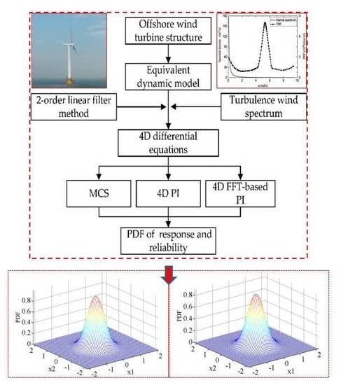
Stochastic dynamic analysis of an offshore wind turbine (OWT) structure plays an important role in the structural safety evaluation and reliability assessment of the structure. In this paper, the OWT structure is simplified as a linear single-degree-of-freedom (SDOF) system and the corresponding joint probability density function (PDF) of the dynamic response is calculated by the implementation of the path integration (PI) method. Filtered Gaussian white noise, which is obtained from the utilization of a second-order filter, is considered as horizontal wind excitation and used to excite the SDOF system. Thus, the SDOF model and the second-order linear filter model constitute a four-dimensional dynamic system. Further, a detailed three-dimensional finite element model is applied to obtain the natural frequency of the OWT and the efficient PI method, which is modified based on the fast Fourier transform (FFT) convolution method, is also utilized to reduce the execution time to obtain the PDF of the response. Two important parameters of wind conditions, i.e., horizontal mean wind speed and turbulence standard deviation, are investigated to highlight the influences on the PDF of the dynamic response and the reliability of the OWT.

1. Introduction

Wind energy has been playing an increasingly important role lately regarding the successful transition from fossil fuels to renewable energy [1]. Offshore wind energy has advantages such as a higher quality of wind resources, a larger suitable free area to develop [2,3], and a smaller influence on the environment (particularly wind turbine noise [4,5,6]) compared with onshore wind energy. In the last few decades, a rapid growth in wind energy development has been witnessed throughout the world [7,8,9]. As in the ocean environment, an offshore wind turbine (OWT) structure is always excited by various random excitations, such as wind, waves, and currents, which all pose a great threat to the structure. Hence, it is a challenge for designers and manufacturers to construct an offshore wind farm [10,11].

Traditionally, code-based designs such as IEC [12], DNVGL [13], and CCS [14] utilize deterministic methods to predict the structural dynamic response. In this regard, the stochastic dynamic response of the OWT can be obtained by one or several deterministic loads or excitations. Moreover, the structural dynamic responses calculated by deterministic methods are normally faster than those by probabilistic (stochastic) methods. However, in many practical structures, a perfect deterministic behavior cannot be guaranteed, not only because of unpredictable excitation, but also because of various uncertainties in the structures. Therefore, dynamic response analysis was implemented in recent studies based on the assumption that some randomness is present in the excitation part [15] and it is of importance for the normal operation and maintenance to ensure the safety of the OWT. To obtain a more accurate dynamic response of the OWT under external excitation, a probability approach can be used to calculate the probability density function (PDF) of the state variables and evaluate the reliability of the OWT.

For dynamic systems, the joint PDFs and joint moments of the state variables can be computed by probabilistic methods [16]. Normally, it is hard to attain the precise joint response PDFs and the transient evolutionary PDF under stochastic excitation [15]. To solve this problem, many approximate methods, such as equivalent linearization [17], the perturbation method [18], and stochastic averaging [19], have been adopted and these replace the original nonlinear system in a probabilistic sense. The methods mentioned above simplify the problem, in which the important nonlinear features of systems were often neglected. Even though these methods can provide stationary or non-stationary response results with an acceptable level of accuracy, for more practical and complex problems, they fail to obtain an analytical solution [20]. In addition, the Monte Carlo simulation (MCS) method is commonly regarded to obtain accurate results and can be used to verify the calculation results extracted from the other approximate methods. Nevertheless, when high dimensions and long-period simulations are encountered, the MCS seems to be impractical because of the large demand of the computational resources and efforts [16]. The probabilistic properties of stochastic dynamic systems are governed by the Fokker–Planck (FP) equation when systems are excited by white noise or filtered white noise [15]. Two research problems on the system’s variable distribution and the corresponding reliability evaluation can be solved based on an accurate joint response PDF, which can be obtained directly by solving the FP equation [20]. Analytical solutions of the FP equation are only obtainable for some linear or limited nonlinear systems, while direct numerical solutions, e.g., via the finite element method [21] and the finite different method [22], suffer from the “curse of dimensionality.” As an alternative, the path integration (PI) method is assumed to be an effective numerical method for the accurate solution of the FP equation [23]. For the PI method, which is based on an iterative method to compute the response PDFs for systems that satisfy Markov properties, the response PDFs are computed by means of a step-by-step solution technique according to the total probability law. Due to the advantage of the PI method in stochastic dynamic analysis, it has already been effectively adjusted for Markov processes to obtain response PDF and system reliability [24,25].

In recent years, many studies have been conducted on the stochastic dynamic response and the reliability of low-dimensional systems with linear or nonlinear restoring forces or damping in order to obtain 2D to 6D state spaces. Alevras and Yurchenko [20] applied the PI approach to analyze high-dimensional dynamic systems (4D to 6D) and accelerate the computation speed of obtaining the joint response PDF by means of a graphics processing unit (GPU). Iourtchenko et al. [26] presented a reliability analysis of strongly nonlinear single-degree-of-freedom (SDOF) systems by the PI approach. Naess and Johnsen [27] applied a 3D PI method to estimate the response PDF of nonlinear and compliant offshore structures. Zhu and Duan [28] evaluated the nonlinear ship-rolling driven by random wave load in random seas by a 4D PI method and verified by the MCS technique. Currently, some 6D problems can be resolved by the PI method with the help of a GPU, while 4D or lower dimension problems can be evaluated by this method at satisfactory computational efforts. Two different main streams are available to obtain the results at an acceptable cost, i.e., the acceleration of computational speed and the reduction of execution efforts. GPU acceleration [20] is put forward to accelerate the computation speed, while techniques such as fast Fourier transform (FFT) [29], decoupling [30], and decomposition [14] can be adapted to lessen the extensive computational resources on the center processing unit (CPU).

Moreover, many pieces of research on the stochastic dynamic characteristics of OWT have also been explored recently from three aspects, including physical model experiments, the finite element method, and analytical solutions. In order to make up for the deficiencies of DNV or API code, which are used to obtain the dynamic response under cyclic loading excitation, Domenico et al. [31] proposed a small scaled model of a monopile wind turbine in kaolin clay soil subjected to cyclic horizontal loading to study the long-term behavior of a system and to quantify the changes in natural frequency and the damping of models using dimensionless parameters, i.e., the length-to-diameter ratio and the cyclic stress ratio. It was concluded based on the experimental results that higher strain levels lead to higher reductions in the natural frequency of the model. However, when the cyclic stress ratio is less than 0.02%, there is practically no degradation in natural frequency. Considering the wind and wave loads, the soil stiffness, and the geometric size of the structure, a comprehensive study on the dynamic behavior of an OWT supported by a monopile in the time domain was investigated by Swagata et al. [32]. It showed that the soil–monopole–tower interaction and soil nonlinearity can increase the responses of the OWT system. Simultaneously, the rotor frequency was found to play a more dominant role than the blade passing frequency and the wave frequency. A new method was proposed to calculate the mean degradation index based on the derivatives of the degradation functions by Woochul et al. [33]. It can be used to significantly decrease the computational effort considering the degradation of the soil modulus of the foundation under stochastic loading conditions. Further, the evolution of the dynamic response should be considered in the design process to secure the serviceability of OWTs and substructures. Considering the soil stiffness and geometric size affecting the dynamic response in clay, Swagata and Sumanta [34] established a dynamic analysis system of the OWT using a beam on a nonlinear Winkler foundation model to address the feasibility of soft–soft and soft–stiff design approaches. It was shown that the main control standard for a wind turbine design in hard clay was the fatigue limit state and fatigue load is a key factor in wind turbine design and stable operation. Damgaard et al. [35] evaluated the extent to which changes in soil properties affect the fatigue loads of one OWT installed on the monopile under parked conditions. More than 30% changes of the soil stiffness, the soil damping, and the presence of sediment transportation at the seabed may occur and were shown to be critical for the fatigue damage equivalent moment at the mudline. In order to accurately estimate the dynamic response of the OWT tower under wind excitation, Feyzollahzadeh et al. [36] proposed an analytical transfer matrix method to determine the wind load response based on Euler–Bernoulli’s beam differential equation. This new method can be used to maintain a higher accuracy in wind-induced vibration analysis compared with conventional numerical methods. Laszlo et al. [37] presented a simplified design procedure for OWT foundations to simplify the design steps and the calculation process based on the site characteristics, the turbine characteristics, and the ground profile. The research example showed that the simplified method arrived at a similar foundation to the one actually used in the London Array wind farm project. The state of practice in seismic design of the OWT and the existing design codes was firstly reviewed by Kaynia [38]. It was indicated that the vertical earthquake excitation makes an obvious influence on the OWTs due to their rather high natural frequencies in the vertical direction. Further, the earthquake loads can be considerably reduced by radiation damping. In order to avoid 1P frequency close to the natural frequency, Saleh et al. [39] proposed analytical solutions to predict the eigenfrequencies of the OWTs supported by the jacket using the finite element method. The ratio of the super-structure stiffness to the vertical stiffness of the foundation and the aspect ratio of the jacket governed the rocking frequency of a jacket. These results have an impact on the choice of foundations for jackets.

This paper focuses on the numerical investigation of the stochastic dynamic analysis of the OWT under horizontal stochastic wind excitation. In Section 2, the dynamic system of the OWT is expressed as a linear SDOF system and the stochastic wind excitation is described as filtered Gaussian white noise by means of the second-order filter technique. Therefore, the 4D PI method is adjusted to obtain the joint PDF of the system’s response, while the marginal PDF of the response variables is obtained by the FFT-based acceleration method to reduce computational efforts. Meanwhile, the results are verified with the generally-used MCS method in Section 3. Furthermore, the influences of horizontal mean wind speed and turbulence intensity on the dynamic response PDF and the reliability of the OWT are explored. It is shown that the FFT-based PI method for the OWT not only provides accurate response statistics distribution at acceptable computation efforts, but also offers an evaluation for reliability under normal operation.

2. Materials and Methods

2.1. Equivalent Dynamic Model of the OWT

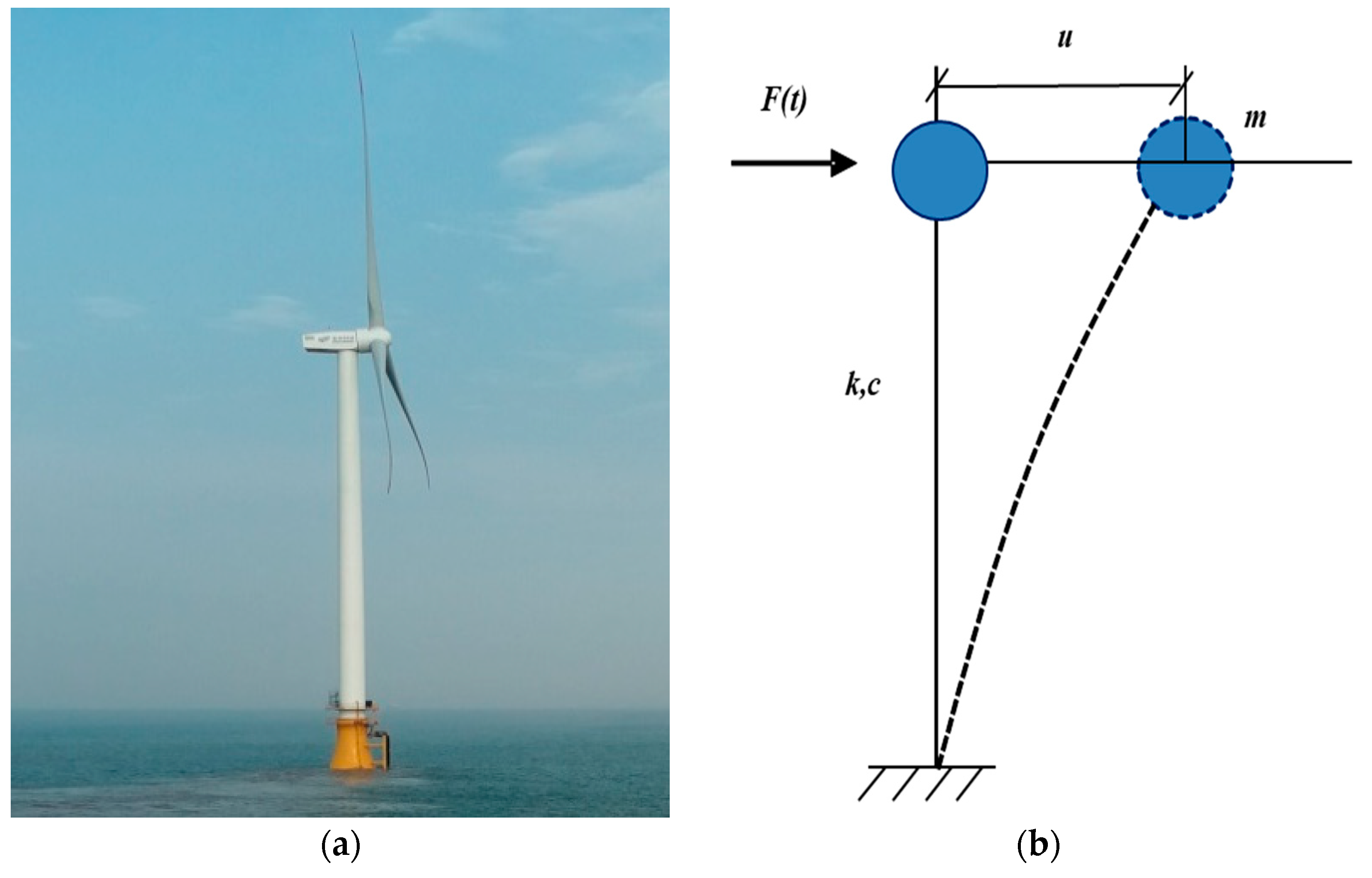
Generally speaking, the rotor-nacelle-assembly (RNA) system and tower of the OWT structure are always considered as the part which is easy to vibrate due to its large slenderness ratio. In this study, the OWT supported by a bucket foundation, as described in Figure 1a, can be simplified as an SDOF system to allow for the stochastic vibrations and the overall mass can be assembled by the concentrated mass method considering the RNA system and the tower. Hence, a simplified model was constructed based on the differential equation of the mass-spring-damping system to describe the structural dynamic response, as shown in Figure 1b.

The motion of the SDOF system can be expressed in the time domain by the following equation [39,40]:

$$m\ddot{u}\left(t\right)+c\dot{u}\left(t\right)+ku\left(t\right)=F\left(t\right),$$

(1)

where m, c, and k are, respectively, the mass, damping, and stiffness of the OWT structure, F(t) is the horizontal stochastic wind excitation, u represents the displacement of the wind turbine, and $\dot{u}$ and $\ddot{u}$ denote the velocity and acceleration, respectively.

Further, Equation (1) can be written as follows:

$$\ddot{u}+2\zeta {\omega }_0\dot{u}+{\omega }_0^{2}u=F/m,$$

(2)

where ${\omega }_0=\sqrt{k/m}$, $c_c=2m{\omega }_0$, and $\zeta =c/c_c$ are, respectively, the undamped natural frequency, critical damping, and damping ratio. There are different sources of damping in the OWT structure, including aerodynamic, hydrodynamic, and material damping. Thus, the overall damping used in this study was referenced the research completed by Bisoi S and Haldar S [34]. The natural frequency ${\omega }_0$ of the OWT structure can be calculated by the finite element model (FEM).

In this study, the horizontal stochastic wind excitation was supposed to be the load acting on the top of the tower expressed by the turbulence wind spectrum. The stochastic wind excitation F can be described by the turbulence wind spectrum S_wind (ω) by the following relationship [41]:

$$S_{FF}\left(\omega \right)={\left|TRF\left(\omega \right)\right|}^2{S}_{wind}\left(\omega \right),$$

(3)

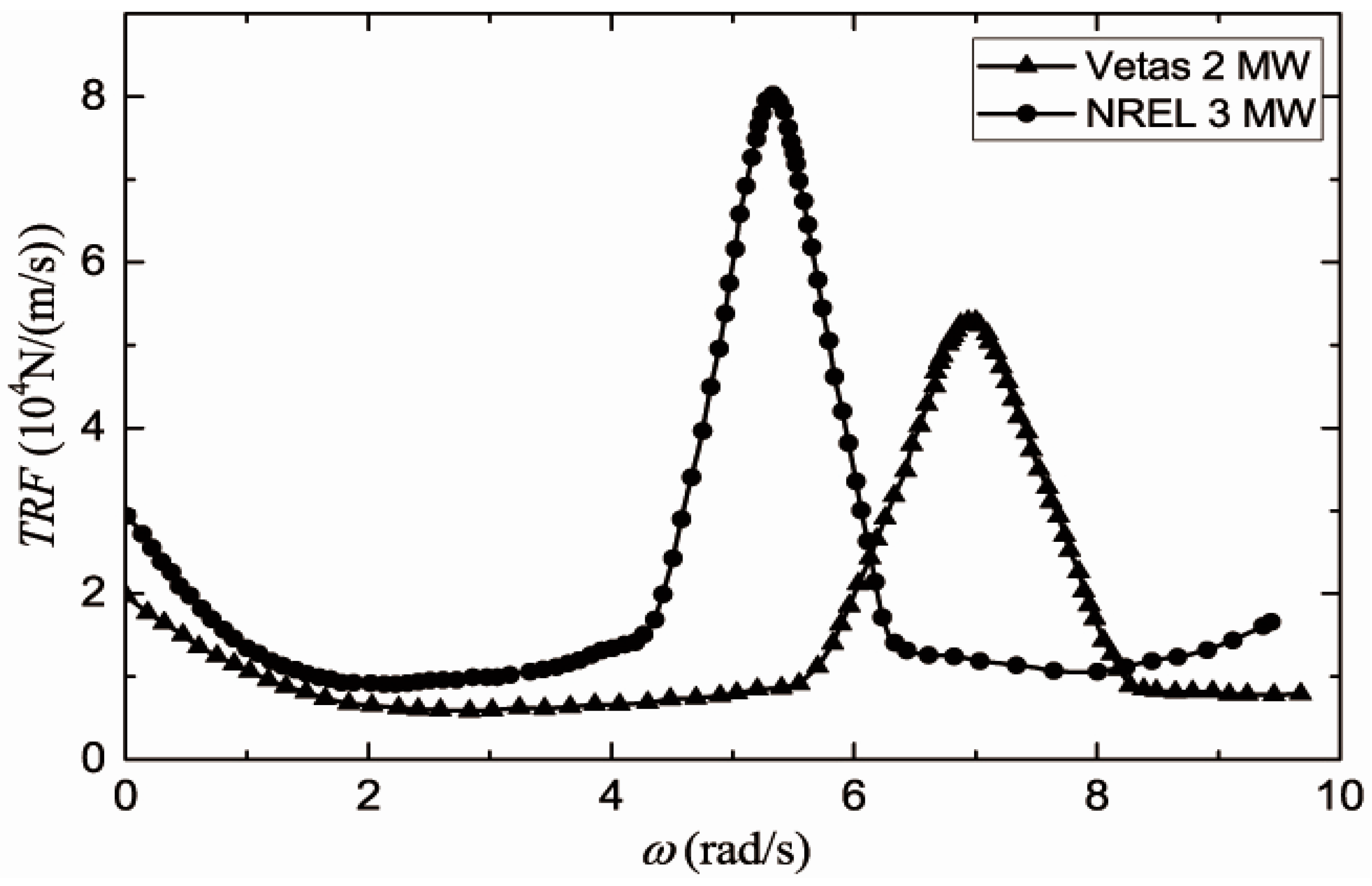
where $S_{FF}\left(\omega \right)$ is the horizontal stochastic wind excitation spectrum and TRF(ω) represents the transfer function of the turbulence wind spectrum to the load spectrum of the top of the tower. For example, the transfer function of the NREL 3 MW wind turbine [41] could be established by scaling the wind transfer function of the Vestas 2 MW wind turbine [42], as shown in Figure 2.

Then, the relative wind excitation spectrum S_ff (ω) can be presented as:

$$S_{ff}\left(\omega \right)={S_{FF}\left(\omega \right)/m}^2.$$

(4)

Transforming Equation (2) to the first order differential equation, the state-space equation can be obtained as follows:

$$\{\begin{array}{l}d{x}_1=x_{2}dt\\ d{x}_2=\left(-2\zeta {\omega }_0{x}_2-{\omega }_0^2{x}_1+x_3\right)dt\end{array},$$

(5)

where $x_1$ and $x_2$ are the horizontal displacement and velocity at the hub, respectively, and $x_3$ is the relative stochastic wind excitation.

2.2. Linear Filter Method for Stochastic Wind

To obtain a filtered white noise from the relative stochastic wind excitation, a second-order linear filter method was utilized for stochastic wind for target spectrum S_ff (ω). The filter method is given by the following differential equations [43]:

$$\{\begin{array}{l}d{x}_3=\left(x_4-\beta x_3\right)dt+\gamma dW\\ d{x}_4=-\alpha x_{3}dt\end{array},$$

(6)

where $x_3$ and $x_4$ are the state variables in the second-order linear filter equations and $x_3$ represents the filtered result of relative wind excitation. $dW=W\left(t+dt\right)-W\left(t\right)$ denotes the increment of a Wiener process. $\alpha$, $\beta$, and $\gamma$ are the parameters of the linear second-order filter method.

The filtered spectrum produced by Equation (6) can be written as:

$$S_{2nd}\left(\omega \right)=\frac{1}{2\pi }\frac{{\gamma }^2{\omega }^2}{{\left(\alpha -{\omega }^2\right)}^2+{\left(\beta \omega \right)}^2},$$

(7)

where $\alpha$, $\beta$, and $\gamma$ can be determined via a least-square algorithm to fit the target spectrum. More details about the filter techniques in a stochastic process can be found in [23,43].

By combining Equations (6) and (7), the 4D dynamic equations were formed. Therefore, the motion of an OWT in wind excitation is represented by the 4D differential equations, which can be written as:

$$\{\begin{array}{l}d{x}_1=x_{2}dt\\ d{x}_2=\left(-2\zeta {\omega }_0{x}_2-{\omega }_0^2{x}_1+x_3\right)dt\\ d{x}_3=\left(x_4-\beta x_3\right)dt+\gamma dW\\ d{x}_4=-\alpha x_{3}dt\end{array}.$$

(8)

It is worth mentioning that the third equation in Equation (8) contains the filtered noise, which indicates the noise input. The 4D differential equations presented a Markov system excited by a filtered white noise, which could be solved by the PI method.

2.3. Finite Element Modeling

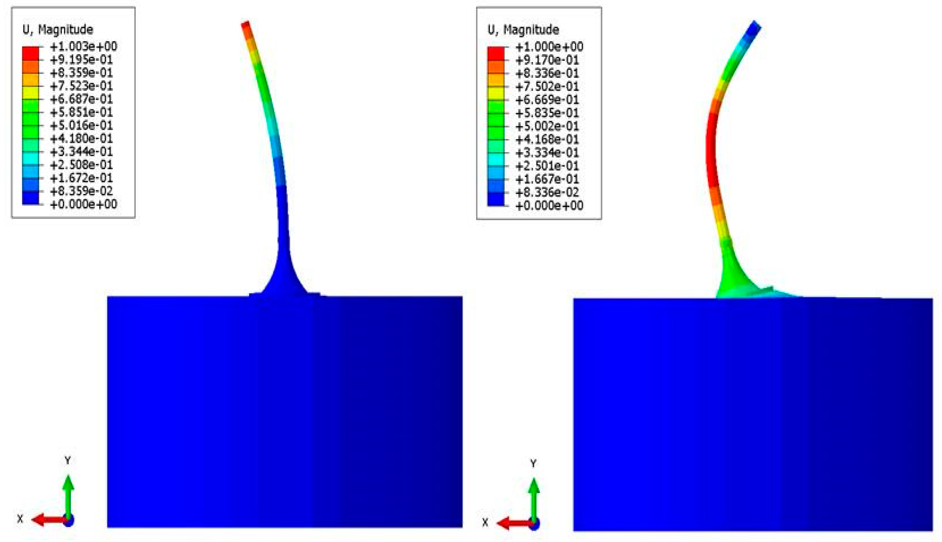
To obtain the natural frequency of an OWT accurately in Equations (2) and (8), a detailed three-dimensional FEM of OWT supported by a bucket foundation was developed, as shown in Figure 3. The parameters came from the OWT with a bucket foundation at Xiangshui offshore wind farm in the Yellow Sea areas of China, as shown in Figure 1a. The bucket foundation consisted of a concrete top and a steel bucket wall with a diameter of 30.0 m and a height of 10 m. The transition part between the bucket foundation and the tower was made of pre-stressed concrete with a gradual diameter from 5.1 to 20 m and a height of 20 m. The radius and height of the soil were 90 and 63.6 m, respectively, to minimize the boundary effect. The physical parameters for the NREL 3 MW turbine listed in

Table 1. Physical parameters of the NREL 3 MW wind turbine.

Parameters	Values
Blade number	3
Hub height above sea level (m)	90
Tower diameter base, top (m)	4.3, 3.2 (linear variation)
Tower thickness base, top (mm)	50, 30 (linear variation)
Rotor-nacelle mass (t)	180
Foundation mass (t)	2700

were used to obtain the transfer function. In the numerical model, an 8-node linear brick element with reduced integration (C3D8R) was used for the three-dimensional solid element for the transition piece, the foundation top, and the soil. Simultaneously, a 2-node linear element (T3D2) was used for the truss element of steel rebar and a 4-node doubly curved thin element (S4R) was used for the shell element for both the tubular steel tower and the foundation wall. Materials include steel, concrete, with the properties listed in

Table 2. Material properties of the steel and concrete.

Material	Young’s Modulus (GPa)	Poisson’s Ratio	Density (kg/m3)
Steel	200.0	0.30	7850
Concrete	36.0	0.20	2500

, and soil were assumed as elastic materials. At the same time, the contact between the bucket foundation and surrounding soil was considered as a contact pair with the characteristics of tangential friction and a small slide approach. According to geological exploration, geological parameters were used for the sea close to the Jiangsu province of China and are shown in

Table 3. Geological parameters used in the finite element model (FEM).

Depth	Young’s Modulus (MPa)	Poisson’s Ratio	Cohesion (kPa)	Friction Angle (°)
12.0	15.0	0.30	9.0	31.0
12.0	31.5	0.35	4.4	33.5
12.2	20.0	0.30	4.7	33.2
13.3	33.0	0.23	10.8	29.1
14.1	39.0	0.25	5.2	33.0

. Boundary conditions of the OWT model are treated with the bottom of the soil fully constrained and the horizontal and vertical directions symmetrically constrained, while the other boundaries of soil foundation are constrained except for the vertical direction. The natural frequencies and mode shapes of the OWT can be found in

Table 4. Structural dynamic properties in modal analysis.

Mode Order	Eigenvalue rad/s	Model
1st	1.98	For-aft
2nd	15.52	For-aft

and Figure 4.

2.4. The Path Integration Method

The PI method was applied to derive the joint PDF for Equation (8), which can be interpreted in the Ito stochastic differential equation (SDE) based on Markovian nature.

Here, Equation (8) satisfied a 4-dimensional (4D) Ito process X and the SDE can be expressed in the following general case:

$$\dot{\mathit{X}}=\mathit{\alpha }\left(\mathit{X},t\right)+\mathit{b}\left(\mathit{X},t\right)\mathit{W}\left(t\right),$$

(9)

where $\mathit{X}={\left(x_1,\cdots ,x_4\right)}^{\mathrm{T}}$ is the 4D state-space vector, $\mathit{\alpha }\left(\mathit{X},t\right)$ is the drift matrix, $\mathit{b}\left(\mathit{X},t\right)$ is the diffusion matrix, and $\mathit{W}\left(t\right)$ is an m-dimensional vector of the independent Gaussian white noise stochastic process.

When the response PDFs at an earlier time instance and the transitional PDFs are already known, the response PDF at a given time instant can be obtained by the following Chapman–Kolmogorov equation:

$$p\left(\mathit{X},t\right)={\displaystyle {\int }_{-\infty }^{\infty }\underset{TransitionPDF}{\underbrace{p\left(\mathit{X},t|{\mathit{X}}^{\prime },t^{\prime }\right)}}}\underset{PreviousPDF}{\underbrace{p\left({\mathit{X}}^{\prime },t^{\prime }\right)}}d{\mathit{X}}^{\prime },$$

(10)

where $t^{\prime }$ is denoted as the time before t and ${\mathit{X}}^{\prime }$ is denoted as the state variable before X.

A state-space discretization and a time discretization, which are grid points at state space as well as a time step t = t′ + Δt, were needed to solve Equation (10). Further, to achieve a greater accuracy of the discretization process, a 4th-order Runge–Kutta–Maruyama (RKM) discretization approximation was applied [10]:

$$\mathit{X}\left(t\right)=\mathit{X}\left(t^{\prime }\right)+\mathit{r}\left(\mathit{X}\left(t^{\prime }\right),t^{\prime }\right)\Delta t+\mathit{b}\left(t^{\prime }\right)\Delta \mathit{W}\left(t^{\prime }\right),$$

(11)

where $\mathit{r}\left(\mathit{X}\left(t^{\prime }\right),t^{\prime }\right)$ is the 4th-order Runge–Kutta approximation and $\Delta \mathit{W}\left(t^{\prime }\right)=\mathit{W}\left(t\right)-\mathit{W}\left(t^{\prime }\right)$ is the increment of the Wiener process. The 4th-order Runge–Kutta scheme was also suitable for the propagation of $\mathit{X}$ forward in time and is denoted by ${\mathit{r}}_j$, $j=1,\cdots ,4.$

When the time step Δt was small enough, the transition probability density (TPD) could be expressed as a degenerate Gaussian distribution, given by the following expressions:

$$\begin{array}{ll}p\left(\mathit{X},t|{\mathit{X}}^{\prime },t^{\prime }\right)=& \delta \left(x_1-{x^{\prime }}_1-r_1\left({\mathit{X}}^{\prime },t^{\prime }\right)\Delta t\right)\times \delta \left(x_2-{x^{\prime }}_2-r_2\left({\mathit{X}}^{\prime },t^{\prime }\right)\Delta t\right)\\ & \times \tilde{p}\left(x_3,t|{\mathit{X}}^{\prime },t^{\prime }\right)\times \delta \left(x_4-{x^{\prime }}_4-r_4\left({\mathit{X}}^{\prime },t^{\prime }\right)\Delta t\right)\end{array}$$

(12)

where

$$\tilde{p}\left(x_3,t|{\mathit{X}}^{\prime },t^{\prime }\right)=\frac{1}{\sqrt{2\pi {\sigma }^2\Delta t}}\exp \left\{-\frac{{\left[x_3-{x^{\prime }}_3-r_3\left({\mathit{X}}^{\prime },t^{\prime }\right)\Delta t\right]}^2}{2{\sigma }^2\Delta t}\right\}.$$

(13)

When the initial PDF at $t^{\prime }=0$ was known, the transient evolution of the PDF of X(t) could be calculated by the iterative algorithm, so the PDF of the system response could be calculated at any time t by repeating this procedure. The initial PDF can be chosen as a Gaussian distribution with the mean and variance extracted by the MCS. The cubic B-spline technique was then applied to interpolation such that the required value could be calculated [23]. A general summary of the PI procedure can be found in Reference [20].

As stated above, to reduce the computation efforts, an FFT-based convolution strategy for the implementation of the PI method was proposed by Mo and Naess [29]. The implementation included the following two steps: (1) Solving the PDF of the deterministic part and the noise input part and (2) convoluting these two parts. An obvious advantage of the FFT-based PI algorithm was that it made use of the FFT algorithm, which requires $O\left(N\log \left(N\right)\right)$ in computational complexity rather than iterating over the full state space [15].

The PDF at the time $t^{\prime }$ and the TPD give a convolution in $\tilde{\mathit{X}}$:

$$p\left({\mathit{X}}^{\prime },t^{\prime }\right)=p\left({\mathit{g}}^{-1}\left(\tilde{\mathit{X}}\right),t^{\prime }\right)\left|{\mathit{J}}_{g^{-1}}\right|,$$

(14)

$$p\left(\mathit{X},t|{\mathit{X}}^{\prime },t^{\prime }\right)=\delta \left(x_1-{\tilde{x}}_1\right)\times \delta \left(x_2-{\tilde{x}}_2\right)\times \delta \left(x_4-{\tilde{x}}_4\right)\times \frac{1}{\sqrt{2\pi {\sigma }^2\Delta t}}\exp \left\{-\frac{{\left(x_3-{\tilde{x}}_3\right)}^2}{2{\sigma }^2\Delta t}\right\},$$

(15)

where ${\tilde{x}}_j={x^{\prime }}_j+r_j\left({\mathit{X}}^{\prime }\right)\Delta t=g_j\left({\mathit{X}}^{\prime }\right)$ and $\mathit{g}={\left(g_1,g_2,\cdots ,g_4\right)}^{\prime }$. $\left|{\mathit{J}}_{g^{-1}}\right|$ is the Jacobi determinant of the backward numerical step and $\delta (\cdot )$ denotes the Dirac delta function symbol.

The result for Equation (9) by combining Equations (14) and (15) is a convolution in ${\tilde{x}}_3$:

$$\tilde{p}\left(\mathit{X}\right)=p\left({\mathit{g}}^{-1}\left(\mathit{X}\right),t^{’}\right)\left|{\mathit{J}}_{g^{-1}}\right|,$$

(16)

$$\tilde{q}\left(\mathit{X}\right)=\delta \left(x_1\right)\times \delta \left(x_2\right)\times \delta \left(x_4\right)\times \frac{1}{\sqrt{2\pi {\sigma }^2\Delta t}}\exp \left\{-\frac{x_3^2}{2{\sigma }^2\Delta t}\right\},$$

(17)

$$p\left(\mathit{X},t\right)=\tilde{p}\left(\mathit{X}\right)\times \tilde{q}\left(\mathit{X}\right),$$

(18)

where the convolution theorem reads

$$h=p\times q\leftrightarrow F\left(h\right)=F\left(p\right)\times F\left(q\right).$$

(19)

In this study, an obvious difference compared with the regular PI method is that one could multiply a 1-dimensional $\left(x_3\right)$ probability distribution in Fourier space and then utilize the inverse transformation. Via the regular PI method, one integrated over the whole state space. The implementation of the FFT convolution can be seen in Figure 5.

Based on the above PDF solutions for the 4D dynamic system, the joint PDF and marginal PDF of response variables of the OWT could be calculated using the regular PI method or the FFT-based PI method. Additionally, the reliability was also an important factor for the safety assessment of the OWT subjected to horizontal stochastic wind excitation, which can be defined with respect to the displacement $x_1$ in the following manner:

$$P\left(x_1\right)={\displaystyle {\int }_{-\infty }^{\infty }{\displaystyle {\int }_{-\infty }^{\infty }{\displaystyle {\int }_{-\infty }^{\infty }{\displaystyle {\int }_{x_l}^{x_u}p\left(x_1,x_2,x_3,x_4\right)d{x}_{1}d{x}_{2}d{x}_{3}d{x}_4}}}},$$

(20)

where $p\left(x_1,x_2,x_3,x_4\right)$ is the joint PDF calculated by the 4D PI method and $x_l$ and $x_u$ are defined as the safe range of displacement representing the lower and upper threshold levels, respectively. Therefore, the probability $P\left(x_1\right)$ was the probability that the displacement $x_1$ stayed between the lower and upper thresholds over three other dimensions. The explicit guideline for the permissible rotation angle or the displacement at the tower top of the OWT was not determined in the recent wind turbine design code [34]. The allowable horizontal displacement at the top of the tower in this study was considered to be 1/75 of the hub height above sea level when linear analysis was conducted [44]. However, Bisoi [34] and Bhattacharya [45] suggested ±5° as the permissible rotation angle at tower top for the wind turbine supported by monopile and floating wind turbine. Hence, this allowable value was also applicable to the OWT supported by the bucket foundation in this study.

3. Results and Discussion

3.1. Stochastic Dynamic Response of the OWT

Based on the equivalent dynamic model, the dynamic response prediction and reliability of the OWT by means of the PI method are discussed in this section. The model of the OWT remains the same during the discussion, while the parameters of wind conditions change according to specific cases. The parameters of horizontal mean wind speed, turbulence standard deviation, and a second-order linear filter for five cases under the different wind conditions are provided in

Table 5. Parameters for the second-order filter for different wind conditions with different horizontal mean wind speeds and turbulence standard deviation.

Cases	Mean Wind Speed Vhub (m/s)	Turbulence Standard Deviation σk (m/s)	Turbulence Intensity I	α	β	γ
Case 1	16	2.884	0.180	0.009	0.134	0.534
Case 2	20	2.472	0.124	0.010	0.140	0.484
Case 3	20	2.884	0.144	0.009	0.141	0.565
Case 4	20	3.296	0.165	0.010	0.139	0.638
Case 5	24	2.884	0.120	0.009	0.145	0.590

. The joint PDFs were extracted by MCS, the PI method, and the FFT-based PI method. Moreover, two important parameters, i.e., the horizontal mean wind speed V_hub and the turbulence standard deviation σ_k, were investigated to highlight the effects on the response PDF and the reliability of the OWT individually.

The OWT supported by the bucket foundation was modeled to predict the wind turbine response under stochastic wind conditions. The main parameters of the OWT structure and the wind conditions are given in Table 1, Table 2 and Table 3. As stated in Table 4, the natural frequency ${\omega }_0$ for the OWT could be calculated by modal analysis of FEM proposed in Section 2.3.

In this work, the spectral density of stochastic wind speed can be represented by the Kaimal spectrum [12,46], which is widely used in design code and research:

$$S_k\left(f\right)={\sigma }_k^2\frac{4L_k/V_{\mathrm{hub}}}{{\left(1+6f{L}_k/V_{\mathrm{hub}}\right)}^{\raisebox{1ex}{$5$}\!\left/ \!\raisebox{-1ex}{$3$}\right.}},$$

(21)

where $f$ is the frequency in Hertz, $S_k$ is the single-sided velocity component spectrum, ${\sigma }_k^2$ is the deviation of the wind speed component, V_hub is the 10 min horizontal mean wind speed at the hub speed in m/s, and L_k is the velocity component integral scale parameter. Turbulence intensity I is defined as the ratio σ_k/V_hub. The categories for higher, medium, and lower turbulence denoted by Class A, B, and C are shown in Figure 6, respectively.

In this section, the specific wind condition of Case 3 with V_hub = 20 m/s and σ_k = 2.88 m/s was selected as an example for the subsequent study. The transfer function for the NREL 3 MW wind turbine under the selected wind condition is presented in Figure 7. It could be observed that transfer function was a broad-band spectrum, while the Kaimal spectrum was a narrow-band spectrum. Furthermore, the spectral density near the natural frequency was relatively small; thus, the OWT was not vibration-sensitive to such wind excitation. Under such circumstances, wind excitation cannot produce the resonance effect for the OWT structure. The relative wind excitation spectrum, which had the same spectral shape as the Kaimal spectrum, is plotted in Figure 7. The wind excitation spectrum and the relative wind excitation spectrum for the different wind conditions could then be determined by Equations (3) and (4), respectively. As stated in Section 2.2, the parameters $\alpha$, $\beta$, and $\gamma$ in the second-order filter expressed by Equation (7) were determined by a least-square algorithm. The fitting results and the target spectrum are shown in Figure 8, which demonstrates that the spectrum generated by the second-order linear filter matched very well with the target spectrum.

All the parameters needed in constituting the 4D differential equation, which was established to describe the dynamic response of the OWT, were determined after performing spectrum fitting. As mentioned above, the joint PDF of the dynamic response of the OWT could be calculated through the 4D PI method. Furthermore, the joint PDF of displacement $x_1$ and velocity $x_2$ was determined by integrating the entire ranges of two other dimensions. In addition, MCS was adapted to solve the corresponding SDE based on the fourth-order RKM method and then to obtain the joint PDFs. In this section, the results extracted from MCS, the PI method, and the FFT-based PI method are respectively denoted as MCS, PI, and FFT-PI, where MCS was generally assumed to be accurate and was used to verify the PI and FFT- PI method.

The joint PDFs of the stationary dynamic response under the selected wind conditions computed by MCS and the regular PI method are shown in Figure 9. It can be observed that the PDFs of the response were symmetrical because both the OWT structure and the distribution of the wind excitation were symmetrical. Based on the joint PDFs, as shown in Figure 9, the second moments were calculated as ${\left(x_1,x_1\right)}_{\mathrm{PI}}=0.168$ and ${\left(x_2,x_2\right)}_{\mathrm{PI}}=0.179$ by the regular PI method, while the MCS results were ${\left(x_1,x_1\right)}_{\mathrm{MCS}}=0.176$ and ${\left(x_2,x_2\right)}_{\mathrm{MCS}}=0.190$. Thus, the relative errors of the second moments were, respectively, 4.5% and 5.8%. Based on the calculated second moments shown in Figure 9, the joint PDFs of the dynamic response extracted from the regular PI method were found to match very well with the results yielded by the MCS. As shown in Figure 10a, the displacement PDFs of PI, FFT-PI, and MCS were compared and the PDFs of displacement $x_1$ based on these three methods were similar. Nevertheless, both the PI and FFT-PI differed slightly from MCS, far from the $x_2=0$ shown in Figure 10b. In this case, these two PI methods provided a satisfactory solution. It is worth noting that times required for the implementation of the code for computing the response PDFs were, respectively, 26,900 s and 4700 s for the regular PI and FFT-based PI methods when 100 time steps were conducted on a personal computer. Hence, it is obvious that the PI code, by the FFT-based PI method, was implemented with great efficiency and computation speed and with acceptable accuracy. In the subsequent study, the FFT-based PI method was chosen first to implement the PI code, which accounted for the computational efforts.

3.2. Parameter Influences of Wind Conditions

In this section, the effects of the horizontal mean wind speed and the turbulence standard deviation on the results extracted from the FFT-based PI method were investigated. Firstly, the effect of horizontal mean wind speed V_hub was studied by introducing three different mean wind speeds with a turbulence intensity fixed to 2.88. Three different horizontal mean wind speeds of 16 m/s, 20 m/s, and 24 m/s were compared in terms of PDFs of displacement (x₁) under stochastic wind excitation, which were respectively considered Case 1, Case 3, and Case 5 in Table 5. The corresponding relative wind excitation spectra for Case 1, Case 3, and Case 5 and the marginal PDF of displacement are displayed in Figure 11a,b, respectively. It is described in Figure 11a that the spectral density from the high mean wind speed was higher than that obtained from the low one, while Figure 11b shows that the marginal PDF from the high mean wind was wider than that calculated from the low one, even though the differences were quite small in these two figures. Thus, it is demonstrated that the horizontal mean wind speed had little influence on the spectral density of wind excitation and the PDFs of responses.

Secondly, three different wind conditions of Case 2, Case 3, and Case 4 were chosen to exhibit the influences of turbulence standard deviation σ_k on the relative wind excitation spectra and the response PDF of the OWT. As indicated in Equation (21), the turbulence standard deviation σ_k was in a square term, whose impact was greater than the mean wind speed. The influence of σ_k on the relative wind excitation was then obvious when considering Equation (3) and Equation (4). After performing the FFT-PI code for the three cases, the joint PDF of displacement of the OWT under stochastic wind excitation could be obtained. The relative wind spectrum of the three cases is given in Figure 11c, while the marginal PDFs of displacement are displayed in Figure 11d. It was observed that the shapes of the PDFs calculated by the FFT-PI method became wider, representing a greater probability of a larger displacement of the OWT and an increase in turbulence standard deviation.

3.3. Reliability Assessment

Based on the joint PDFs and Equation (20), the reliability of the OWT response was obtained. The response reliability of the OWT under five different wind conditions is listed in

Table 6. Reliability for five different wind conditions.

Cases	Case 1	Case 2	Case 3	Case 4	Case 5
Reliability (%)	99.84	99.90	99.75	99.41	99.71

. It can be observed that, among the five cases, Case 4 yielded the lowest reliability, while Case 2 showed the highest reliability. In this study, with the increase in wind speed or turbulence standard deviation, the reliabilities decreased differently. For example, based on Case 1, 3, and 5, the reliabilities declined steadily, while there was a noticeable and quick fall in reliability in Case 2, 3, and 4.

A reasonable conclusion that can be drawn is that the 4D PI method can be applied as an effective and efficient alternative to obtain a joint PDF of a dynamic response with the assistance of FFT convolution. The influences of wind condition parameters, i.e., horizontal mean wind speed and turbulence standard deviation, on both joint PDFs and the reliability of OWT responses, were evaluated and it is shown that the influence of turbulence standard deviation is comparatively greater than that of the horizontal mean wind speed.

4. Conclusions

In this paper, an effective and accurate path integration (PI) method, based on Markov properties and fast Fourier transform (FFT) convolution, was implemented to study the stochastic dynamic response of an offshore wind turbine (OWT) structure supported by a bucket foundation under horizontal stochastic wind excitation. More specifically, the OWT structure was assumed to be a single-degree-of-freedom (SDOF) system excited by horizontal wind and the second-order filter was utilized to obtain filtered Gaussian white noise, which resulted in a 4D dynamic system. The FFT was utilized to convert the path integration over the state space to a convolution. The main conclusions that can be drawn are as follows:

• The stochastic dynamic analysis of the OWT under horizontal stochastic wind excitation was numerically investigated by the PI method. The probability density function (PDF) of the joint response obtained by the 4D regular PI and FFT-based PI methods coincided very well with that of the Monte Carlo simulation (MCS), which demonstrated that these two PI methods provide reliable and reasonable results for such a dynamic system describing the OWT.
• The FFT-based PI method held advantages over the MSC and regular PI methods considering computation efficiency and accuracy. Meanwhile, the reliability based on the marginal PDF of displacement and the total probability law could be calculated when the OWT was subjected to stochastic wind excitation.
• The influences of the horizontal mean wind speed and turbulence standard deviation on the relative wind excitation spectrum and the joint PDFs were also investigated. The turbulence standard deviation had a comparatively larger impact than that of horizontal mean wind speed in this study. Therefore, when one assesses the safety of an OWT under horizontal stochastic excitation, turbulence standard deviation is one of the most important aspects that should be taken into account.

References

- Wang, X.; Zeng, X.; Li, J.; Yang, X.; Wang, H. A review on recent advancements of substructures for offshore wind turbines. Energy Convers. Manag. 2018, 158, 103–119. [Google Scholar] [CrossRef]
- Ahmed, N.A.; Cameron, M. The challenges and possible solutions of horizontal axis wind turbines as a clean energy solution for the future. Renew. Sustain. Energy Rev. 2014, 38, 439–460. [Google Scholar] [CrossRef]
- Esteban, M.D.; Diez, J.J.; López, J.S.; Negro, V. Why offshore wind energy? Renew. Energy 2011, 36, 444–450. [Google Scholar] [CrossRef] [Green Version]
- Luca, F.; Stefano, C.; Gaetano, L. A procedure for deriving wind turbine noise limits by taking into account annoyance. Sci. Total Environ. 2019, 648, 728–736. [Google Scholar] [CrossRef]
- Fredianelli, L.; Gallo, P.; Licitra, G.; Stefano, C. Analytical assessment of wind turbine noise impact at receiver by means of residual noise determination without the wind farm shutdown. Noise Control Eng. J. 2017, 65, 417–433. [Google Scholar] [CrossRef]
- Michaud, D.S.; Feder, K.; Keith, S.E.; Voicescu, S.A. Exposure to wind turbine noise: Perceptual responses and reported health effects. J. Acoust. Soc. Am. 2016, 139, 1443–1454. [Google Scholar] [CrossRef] [Green Version]
- Snyder, B.; Kaiser, M.J. A comparison of offshore wind power development in europe and the U.S.: Patterns and drivers of development. Appl. Energy 2009, 86, 1845–1856. [Google Scholar] [CrossRef]
- Michalak, P.; Zimny, J. Wind energy development in the world, Europe and Poland from 1995 to 2009; current status and future perspectives. Renew. Sustain. Energy Rev. 2011, 15, 2330–2341. [Google Scholar] [CrossRef]
- Hong, L.; Möller, B. Offshore wind energy potential in China: Under technical, spatial and economic constraints. Energy 2011, 36, 4482–4491. [Google Scholar] [CrossRef] [Green Version]
- Piasecka, I.; Tomporowski, A.; Flizikowski, J.; Kruszelnicka, W.; Kasner, R.; Mroziński, A. Life Cycle Analysis of Ecological Impacts of an Offshore and a Land-Based Wind Power Plant. Appl. Sci. 2019, 9, 231. [Google Scholar] [CrossRef]
- Seyr, H.; Muskulus, M. Decision Support Models for Operations and Maintenance for Offshore Wind Farms: A Review. Appl. Sci. 2019, 9, 278. [Google Scholar] [CrossRef]
- International Electrotechnical Commission. Wind turbines—Part 1: Design requirements, IEC 61400-1; IEC: Geneva, Switzerland, 2005. [Google Scholar]
- DNVGL. DNVGL-ST-0126: Support Structures for Wind Turbines; DNV GL: Oslo, Norway, 2016. [Google Scholar]
- CCS. Specification for Offshore Wind Turbine Certification; CCS: Beijing, China, 2012. [Google Scholar]
- Mo, E. Nonlinear Stochastic Dynamics and Chaos by Numerical Path Integration. Ph.D. Thesis, Norwegian University of Science and Technology, Trondheim, Norway, 2008. [Google Scholar]
- Narayanan, S.; Kumar, P. Numerical solutions of Fokker–Planck equation of nonlinear systems subjected to random and harmonic excitations. Probabilist. Eng. Mech. 2012, 27, 35–46. [Google Scholar] [CrossRef]
- Sun, Y.; Kumar, M. Numerical solution of high dimensional stationary Fokker–Planck equations via tensor decomposition and Chebyshev spectral differentiation. Comput. Math. Appl. 2014, 67, 1960–1977. [Google Scholar] [CrossRef]
- Crandall, S.H. Perturbation techniques for stochastic vibration of nonlinear systems. J. Acoust. Soc. Am. 1963, 35, 1700–1705. [Google Scholar] [CrossRef]
- Khasminskii, R.Z. A limit theorem for the solutions of differential equations with random right-hand sides. Theor. Probab. Appl. 1966, 11, 390–406. [Google Scholar] [CrossRef]
- Alevras, P.; Yurchenko, D. GPU computing for accelerating the numerical Path Integration approach. Comput. Struct. 2016, 171, 46–53. [Google Scholar] [CrossRef] [Green Version]
- Spencer, B.F.; Bergman, L.A. On the numerical solution of the Fokker-Planck equation for nonlinear stochastic systems. Nonlinear Dynam. 1993, 4, 357–372. [Google Scholar] [CrossRef]
- Wojtkiewicz, S.F.; Johnson, E.A.; Bergman, L.A.; Grigoriu, M.; Spencer, B.F. Response of stochastic dynamical systems driven by additive Gaussian and Poisson white noise: Solution of a forward generalized Kolmogorov equation by a spectral finite difference method. Comput. Method Appl. Mech. Eng. 1999, 168, 73–89. [Google Scholar] [CrossRef]
- Chai, W.; Naess, A.; Leira, B.J. Filter models for prediction of stochastic ship roll response. Probabilist. Eng. Mech. 2015, 41, 104–114. [Google Scholar] [CrossRef]
- Yurchenko, D.; Alevras, P. Stochastic Dynamics of a Parametrically base Excited Rotating Pendulum. Procedia Iutam 2013, 6, 160–168. [Google Scholar] [CrossRef] [Green Version]
- Yurchenko, D.; Iwankiewicz, R.; Alevras, P. Control and dynamics of a SDOF system with piecewise linear stiffness and combined external excitations. Probabilist. Eng. Mech. 2014, 35, 118–124. [Google Scholar] [CrossRef]
- Iourtchenko, D.V.; Mo, E.; Naess, A. Response probability density functions of strongly non-linear systems by the path integration method. Int. J. Non-Lin. Mech. 2006, 41, 693–705. [Google Scholar] [CrossRef]
- Naess, A.; Johnsen, J.M. Response statistics of nonlinear, compliant offshore structures by the path integral solution method. Probabilist. Eng. Mech. 1993, 8, 91–106. [Google Scholar] [CrossRef]
- Zhu, H.T.; Duan, L.L. Probabilistic solution of non-linear random ship roll motion by path integration. Int. J. Non-Lin. Mech. 2016, 83, 1–8. [Google Scholar] [CrossRef]
- Mo, E.; Naess, A. Efficient path integration by FFT. Presented at the 10th International Conference on Applications of Statistics and Probability in Civil Engineering (ICASP10), Tokyo, Japan, 31 July–3 August 2007. [Google Scholar]
- Beylkin, G.; Mohlenkamp, M.J. Algorithms for Numerical Analysis in High Dimensions. SIAM J. Sci. Comput. 2005, 26, 2133–2159. [Google Scholar] [CrossRef] [Green Version]
- Lombardi, D.; Bhattacharya, S.; Muir Wood, D. Dynamic soil–structure interaction of monopile supported wind turbines in cohesive soil. Soil Dyn. Earthq. Eng. 2013, 49, 165–180. [Google Scholar] [CrossRef]
- Bisoi, S.; Haldar, S. Dynamic analysis of offshore wind turbine in clay considering soil–monopile–tower interaction. Soil Dyn. Earthq. Eng. 2014, 63, 19–35. [Google Scholar] [CrossRef]
- Nam, W.; Oh, K.-Y.; Epureanu, B.I. Evolution of the dynamic response and its effects on the serviceability of offshore wind turbines with stochastic loads and soil degradation. Reliab. Eng. Syst. Saf. 2019, 184, 151–163. [Google Scholar] [CrossRef]
- Bisoi, S.; Haldar, S. Design of monopile supported offshore wind turbine in clay considering dynamic soil–structure-interaction. Soil Dyn. Earthq. Eng. 2015, 73, 103–117. [Google Scholar] [CrossRef]
- Damgaard, M.; Andersen, L.V.; Ibsen, L.B. Dynamic response sensitivity of an offshore wind turbine for varying subsoil conditions. Ocean Eng. 2015, 101, 227–234. [Google Scholar] [CrossRef]
- Feyzollahzadeh, M.; Mahmoodi, M.J.; Yadavar-Nikravesh, S.M.; Jamali, J. Wind load response of offshore wind turbine towers with fixed monopile platform. J. Wind Eng. Ind. Aerdodyn. 2016, 158, 122–138. [Google Scholar] [CrossRef]
- Arany, L.; Bhattacharya, S.; Macdonald, J.; Hogan, S.J. Design of monopiles for offshore wind turbines in 10 steps. Soil Dyn. Earthq. Eng. 2017, 92, 126–152. [Google Scholar] [CrossRef] [Green Version]
- Kaynia, A.M. Seismic considerations in design of offshore wind turbines. Soil Dyn. Earthq. Eng. 2018. [Google Scholar] [CrossRef]
- Jalbi, S.; Nikitas, G.; Bhattacharya, S.; Alexander, N. Dynamic design considerations for offshore wind turbine jackets supported on multiple foundations. Mar. Struc. 2019, 67, 102631. [Google Scholar] [CrossRef]
- Chengxi, L. Numerical Investigation of a Hybrid Wave Absorption Method in 3D Numerical Wave Tank. CMES Comput. Model. Eng. Sci. 2015, 107, 125–153. [Google Scholar]
- Yeter, B.; Garbatov, Y.; Guedes Soares, C. Fatigue damage assessment of fixed offshore wind turbine tripod support structures. Eng. Struct. 2015, 101, 518–528. [Google Scholar] [CrossRef]
- Vestas. V80-2MW OptiSpeedTM Offshore Wind Turbine. Available online: http://www.vestas.dk/ (accessed on 10 January 2019).
- Dostal, L.; Kreuzer, E. Probabilistic approach to large amplitude ship rolling in random seas. Proc. Inst. Mech. Eng. Part C J. Mech. Eng. Sci. 2011, 225, 2464–2476. [Google Scholar] [CrossRef] [Green Version]
- Ministry of Housing and Urban-Rural Development of the People’s Republic of China. Code for Design of High-Rising Structures; China Planning Press: Beijing, China, 2006.
- Bhattacharya, S. Challenges in Design of Foundations for Offshore Wind Turbines. Eng. Tech. Ref. 2014. [Google Scholar] [CrossRef]
- DNV. Offshore Standard DNV-OS-J101 Design of Offshore Wind Turbine Structures; DNV: Høvik, Norway, 2014. [Google Scholar]
Figure 1.
Prototype and equivalent dynamic model of the offshore wind turbine (OWT). (a) The OWT supported by bucket foundation; (b) the equivalent dynamic model of the OWT.
Figure 2.
Transfer function (TRF) from wind speed to tower-top load [41].
Figure 3.
The finite element model (FEM) of OWT supported by bucket foundation.
Figure 4.
The first two mode shapes obtained from the modal analysis.
Figure 5.
Implementation procedure of fast Fourier transform (FFT) convolution for Probability density function (PDF).
Figure 6.
Turbulence standard deviation for the normal turbulence model (NTM) [12].
Figure 7.
Wind excitation spectrum for the wind condition of Case 3 and transfer function (TRF) for the NREL 3 MW wind turbine.
Figure 8.
Relative wind excitation spectrum (Sff) and the second-order filtered spectrum for the wind condition of Case 3.
Figure 9.
Joint probability density functions (PDFs) of (x1, x2) extracted from the regular path integration (PI) method and from the Monte Carlo simulation (MCS) for the wind condition of Case 3: (a) Joint PDFs from the regular PI method; (b) joint PDFs from the MCS.
Figure 10.
Marginal PDFs of (displacement, velocity): (a) PDFs of displacement; (b) PDFs of velocity.
Figure 11.
Relative wind excitation spectra and PDF of displacement calculated by FFT-PI for different cases: (a) Relative wind excitation spectral density for Case 1, 3, and 5; (b) PDF of displacement calculated by FFT-PI for Case 1, 3, and 5; (c) Relative wind excitation spectral density for Case 2, 3, and 4; (d) PDF of displacement calculated by FFT-PI for Case 2, 3, and 4.