Article

Effects of a Delayed Expansion of Interconnector Capacities in a High RES-E European Electricity System

1
Öko-Institut e.V., Merzhauser Straße 173, 79100 Freiburg, Germany
2
Bremen Energy Research, Jacobs University Bremen, Campus Ring 1, 28759 Bremen, Germany
*
Author to whom correspondence should be addressed.
Energies 2019, 12(16), 3098; https://doi.org/10.3390/en12163098
Submission received: 28 June 2019 / Revised: 6 August 2019 / Accepted: 7 August 2019 / Published: 12 August 2019
(This article belongs to the Special Issue 100% Renewable Energy Transition: Pathways and Implementation)

Abstract

:
In order to achieve a high renewable share in the electricity system, a significant expansion of cross-border exchange capacities is planned. Historically, the actual expansion of interconnector capacities has significantly lagged behind the planned expansion. This study examines the impact that such continued delays would have when compared to a strong interconnector expansion in an ambitious energy transition scenario. For this purpose, scenarios for the years 2030, 2040, and 2050 are examined using the electricity market model PowerFlex EU. The analysis reveals that both CO2 emissions and variable costs of electricity generation increase if interconnector expansion is delayed. This effect is most significant in the scenario year 2050, where lower connectivity leads roughly to a doubling of both CO2 emissions and variable costs of electricity generation. This increase results from a lower level of European electricity trading, a curtailment of electricity from a renewable energy source (RES-E), and a corresponding higher level of conventional electricity generation. Most notably, in Southern and Central Europe, less interconnection leads to higher use of natural gas power plants since less renewable electricity from Northern Europe can be integrated into the European grid.

Graphical Abstract

1. Introduction

With the signing of the United Nations Paris Agreement on 12 December 2015, 195 states or associations of states [1] committed themselves to limiting global warming to well below 2° C when compared to the pre-industrial level [2]. To implement this goal, the European Commission (EC) presented its 2050 long-term strategy on 28 November 2018 [3]. In this document, the goal of a climate-neutral European economy for the year 2050 is outlined. In order to achieve this goal, a significant expansion of renewable energies especially in the electricity sector must be achieved [4]. For the electricity sector, most scenarios assume that a focus will be on the expansion of technologies providing electricity from renewable energy sources (RES-E) such as solar and wind [5,6,7]. Several studies have shown that an improved spatial distribution of RES-E capacities within Europe is helpful to balance the fluctuations of wind flow and solar radiation [8,9,10].
In 2017, the European Commission agreed to implement the European Energy Union [11]. This strategy consists of five dimensions: energy security, a fully-integrated internal energy market, energy efficiency, decarbonization, and research. An important component for achieving the Energy Union is the expansion of European electricity transmission capacities [12]. In Reference [13], the European Commission already reported in detail on the state of the internal energy market and pointed out that sufficient cross-border transmission capacities are a necessary requirement for achieving the energy policy goals. The advantages resulting from the expansion of the European transmission grid are also described in a large number of studies. Expansion of the transmission grid is being described as a "no regret" strategy [14], an efficient flexibility option [15], a requirement for a cost-efficient RES-E extension and integration [16,17], and as “needed to achieve the European targets cost-efficiently” [18].
However, the EU Commission has also pointed out the stalling of the expansion of interconnector capacities. This hampers the continued development of the internal energy market. On behalf of the EU Commission, Roland Berger Strategy Consultants [19] identified the regulatory framework as a major obstacle to the expansion of cross-border transmission capacity. In addition to regulatory issues, Battaglini et al. [20] also indicate a lack of public acceptance as a cause for the delay in grid expansion. In 2014, the EU Commission launched a package of measures called "Connecting Europe Facility" to improve investment conditions. These measures notably aim at improving and harmonizing approval procedures and adapting regulatory regimes with particular emphasis on dealing with risks in network expansion. The Agency for the Cooperation of Energy Regulators (ACER) has identified significant delays in the projects of common interest (PCI). ACER [21] has shown that 75% of PCIs in the phase of “permitting” are delayed or have been rescheduled.
Many studies compare different levels of grid expansion while maintaining CO2 reduction [8,14] or RES-E targets [17,22,23], to determine the cost-optimal mix through a variation in the expansion of RES-E technologies, back-up capacities, or storage units. As part of the Ten-Year Network Development Plan (TYNDP) 2018, a "no grid" scenario was conducted for the year 2040, in which no further grid expansion is assumed after 2020. All other input data, such as power plant fleet or electricity demand, were kept corresponding to the reference scenario. The authors conclude that “No Grid is incompatible with the achievements of European emission targets” [24]. An additional 156 TWh of RES-E is curtailed per year on average across the scenarios considered and “the grid built between 2020 and 2040 allows a further 10% decrease in power sector CO2 emissions as compared to the 1990 levels” [24].
The present paper focuses on the delay of interconnector expansion and analyzes what impact a persistence of current delays in the expansion of interconnector capacities would have in a high RES-E scenario. The focus is on quantifying the effects of delay of interconnector expansion on the indicators’ CO2 emissions, generation mix, electricity exchange, and variable costs of electricity generation. Scenario years 2030, 2040, and 2050 are being considered with RES-E shares in electricity demand of 62% to 99%. Results show that both CO2 emissions and variable costs of electricity generation increase in case of delayed interconnector expansion. This effect is most significant in scenario year 2050, where lower connectivity roughly leads to a doubling of both CO2 emissions and variable costs of electricity generation. Those effects arise from lower levels of European electricity trading, higher RES curtailment, and corresponding higher conventional electricity generation. With regard to the latter, the analysis indicates a more extensive use of natural gas power plants, especially in Southern and Central Europe, since less renewable electricity from Northern Europe can be integrated.
Section 2 describes methodology and data, including the electricity market model PowerFlex EU, which was used for this analysis. This also includes a review of existing scenarios regarding electricity demand, generation capacities, and net transfer capacities (NTC). The section also explains how the delays in NTC expansion have been derived. The modeling results can be found in Section 3. In Section 4, the results are being discussed and compared with other studies. Lastly, Section 5 concludes.

2. Methodology and Data

This paper examines in a what-if analysis what impact the persistence of current delays in the expansion of interconnector capacities would have in a high RES-E scenario. Electricity market scenarios from various literature sources were evaluated to determine future generation capacities and electricity demand. An ambitious energy transition scenario was derived from these data (cf. Section 2.2). To determine the effects of delayed interconnector expansion, the electricity market scenario was modelled with two different interconnector capacity expansion levels. The high connectivity (HiCon) scenario, with strong interconnector expansion, is based on literature values. The lower connectivity (LowCon) scenario was derived by extrapolating the current interconnector expansion delay (cf. Section 2.3).
For this study, scenario years 2030, 2040, and 2050 were considered. The data described was used as input for the electricity market model PowerFlex EU (see Section 2.1). The effect of a delayed expansion was determined with a delta analysis in which the scenarios high connectivity and lower connectivity were compared.
The following indicators were analyzed:
  • CO2 emissions.
  • Electricity generation mix.
  • Import, export, and transit flows.
  • Variable costs of electricity generation.

2.1. General Model Description-PowerFlex EU

PowerFlex EU is a bottom-up partial model of the European power sector that has been applied in a range of consultancy and research projects on a German and European level, such as analysis on flexibility options [25,26] or scenario development [27,28]. It calculates the dispatch of thermal power plants, feed-in from renewable energy sources, and utilization of flexibility and storage options at minimal costs to meet electricity demand and reserve capacity requirements.
The model covers all ENTSO-E member states except Iceland and Cyprus. A transport model approach is used to represent electricity exchange between countries. For each individual country, a homogeneous market area without grid constraints is assumed. Exchange between countries is limited by net transfer capacities (see Section 2.3).
For Germany, thermal power plants with capacities exceeding 100 MW are represented as individual units. For other countries, the thermal power plant fleet is represented as aggregated vintage classes concerning age, fuel type, and technology of the individual plants.
The available electricity produced from run-of-river, offshore wind, onshore wind, and photovoltaic systems is represented by generic feed-in patterns in hourly resolution. The actual quantity of feed-in is determined endogenously, with the result that the available yield of fluctuating electricity can also be curtailed (e.g., in the case of negative residual load and insufficient storage capacity).
The model considers reservoir hydro plants, pumped hydro storage, battery storage, and power-to-gas (PtG) as flexibility options. The flexibility of reservoir hydro plants is modeled with an inflow profile of hydro in hourly resolution, a storage capacity of the reservoir, a given level of the reservoir for the first and the last time step, and an electrical capacity of the turbine. All other flexibility options mentioned are modeled with the following parameter’s set: pumping or charging capacity, storage capacity, electrical capacity of the turbine or discharging, and the overall efficiency rate. Power–to-gas is modeled as an electricity to electricity storage option to keep the system boundary closed to the electricity system.
The available battery capacities scale with the installed photovoltaic (PV) capacities, and the available capacities of the electrolysers for Power-to-Gas (PtG) generation scale with variable RES-E capacities installed (for details, see Appendix B).
Heat sector coupling is modelled as a further flexibility option only for Germany and not for other ENTSO-E countries. It is represented by combined heat and power plants (CHP) that can shift their power-to-heat ratio within certain technological limitations. Additional generation and flexibility options in the heat sector include heat storage, electrical heating rods, and gas fired boilers.
Electricity demand is assumed to be inelastic. To derive demand profiles in hourly resolution, a standardized demand profile of the base year 2016 is scaled up using scenario-specific annual demand data (see Section 2.2.1). It is assumed that the load profile shape does not change over time (e.g., by increasing demand of new consumers and sector coupling).
Generation, transmission, and storage capacities are determined exogenously, i.e., the model does not endogenously calculate cost efficient investment or divestment pathways. The model assumes perfect foresight and calculates the cost-minimizing dispatch of given capacities in hourly resolution across a single year (8760 hours). In technical terms, it is formulated as a linear optimization problem, implemented in GAMS, and solved using the CPLEX solver.

2.2. Electricity Market Scenarios

In the following sections, the data used is described. All data used has been published (cf. Appendix A). The input data for Germany is based on the scenario Klimaschutzszenario 95 (KS 95) from Reference [28] and is described in Section 2.2.2. To derive the European input data, a scenario analysis based on a literature review was carried out (cf. Section 2.2.1). In Appendix D, the generation capacities per country, used as model input for the year 2050 are given.

2.2.1. European Scenario

The European scenario was determined by means of a scenario analysis of literature data, including TYNDP 2018 [5], the study eHighway 2050 [29], EU Vision Scenario 2017 [30], and EU Reference Scenario 2016 [31]. In the project Model-Based Scenario Analysis of Developments in the German Electricity System, which takes into account the European context up to 2050 in which this study was carried out. Two European electricity market scenarios were derived: an ambitious scenario in which a strong expansion of RES and a significant decline in conventional power plants are assumed, and an unambitious scenario with much slower progress in European energy transition. The unambitious scenario is based on the EU Reference Scenario 2016 [31]. Non EU28 countries are not covered in the scenario and were taken from TYNDP 2018 scenario Sustainable Transition [5].
The years 2040 and 2050 of the ambitious scenario are based on eHighway 2050 scenario 100% RES [29]. Hydro power and biomass generation capacities increase very strongly in the scenario, which does not seem comprehensible from the perspective of natural restrictions, respectively, and competing land use. Therefore, values of the eHighway 2050 Big & Market scenario [29] were used for these technologies. For hydro power generation capacities, it was further assumed that the installed capacities per country will not fall below the current level. In order to ensure that sufficient secure services are available, the size of natural gas capacities, which decrease significantly in the 100% RES scenario, was also taken from eHighway 2050 scenario Big & Market. The data for the scenario year 2030 was generated on the basis of an interpolation between TYNDP 2018 scenario Best Estimate 2020 [5] and the values of the ambitious scenario for the year 2040. In the following, the ambitious and the unambitious scenario are compared with the spread of the considered scenarios. In Appendix C, the scenarios considered are presented in more detail.
Since the European grid expansion will play an important role especially for a high RES-E scenario with large shares of wind and solar, this paper focuses on the ambitious scenario. Further results from this project, such as the effects obtained in the variation of European scenarios while maintaining the German scenario, will be published as a working paper on www.oeko.de by the end of 2019.
The following scenario presentation focuses on EU28 countries, since some of the scenarios only cover these countries. All ENTSO-E member states, except Iceland and Cyprus, were taken into account in the modeling work.
Electricity Demand
Figure 1 shows the development of electricity demand in the unambitious and the ambitious scenario when compared to the scenario spread that results from the scenarios TYNDP 2018 [5], the study eHighway 2050 [29], EU Vision Scenario 2017 [30], and the EU Reference Scenario 2016 [31]. During the period up to 2050, most of the scenarios show a significant increase in demand, which can be attributed to an overcompensation of efficiency measures by an increase of new electricity consumers, such as electric mobility or heat pumps. The unambitious and ambitious scenarios show a relatively similar trend for electricity demand and are in the midfield of the scenarios considered. Compared to 2016, the electricity demand increases by 28% in the unambitious scenario and by 31% in the ambitious one.
Renewable Generation Capacities
Figure 2 shows the development of generation capacities for wind, solar, biomass, and hydro power in the unambitious and the ambitious scenario compared to the scenario spread that results from the scenarios TYNDP 2018 [5], the study eHighway 2050 [29], EU Vision Scenario 2017 [30], and EU Reference Scenario 2016 [31].
Wind and solar capacities increase significantly in all scenarios. The ambitious scenario is located at the top and the unambitious scenario is located at the bottom of the scenario funnel. In the ambitious scenario, wind capacities are more than five times higher than in 2016, and solar capacities are more than six times higher. In the unambitious scenario, wind capacities more than double compared to 2016 and solar capacities almost triple compared to 2016. In the unambitious and the ambitious scenario, both biomass capacities roughly double when compared to 2016. Compared to the scenario spread, this is a moderate increase. Hydro power capacities increase compared to 2016 by approximately 50% in the ambitious scenario and by approximately 10% in the unambitious scenario.
Conventional Generation Capacities
Figure 3 shows the development of the conventional generation technologies natural gas, coal, and nuclear power in the unambitious and the ambitious scenario when compared to the scenario spread that results from the scenarios TYNDP 2018 [5], the study eHighway 2050 [29], EU Vision Scenario 2017 [30], and the EU Reference Scenario 2016 [31]. In most scenarios, natural gas capacities show a slight decline over the next few years, which is followed by an increase until 2050 to provide for sufficient secured capacity. In the ambitious scenario, natural gas capacities in 2050 are approximately 15% above today’s level. In the unambitious scenario, natural gas capacities increase by approximately 25% compared to today’s level.
In all scenarios, coal capacities decline significantly from the current level, even though levels reached in the scenario year 2050 differ significantly. While the ambitious scenario assumes a European-wide phase-out of coal by 2050, the unambitious scenario assumes that coal capacities will decline to approximately 35% by 2040 compared to 2016 and to approximately 33% by 2050.
The scenarios differ even more in the assumptions on nuclear power development. While some scenarios assume an increase in nuclear power, most scenarios assume at least a slight decline. In the unambitious scenario, nuclear power capacities decline to approximately 77% for today’s level. In the ambitious scenario, a European-wide nuclear phase-out is assumed.

2.2.2. German Scenario

The assumptions on the development of the German electricity market are based on scenario Klimaschutzszenario 95 (KS 95) from Reference [28]. Figure 4 shows the development of installed capacities and electricity demand for Germany. In order to end up with a more ambitious scenario in our analysis, we decided to further reduce the coal capacity for 2050 from 2.7 GW to 0 GW compared to the original scenario values. The nuclear phase-out [34] will be completed before 2030. By the year 2050, the installed wind capacity is expected to increase by a factor of 4 compared to the 2016 level and the solar capacity is expected to triple during this period. While biomass in the electricity sector will be of less importance, it is assumed that the installed capacities of hydro power (run-of-river and pumped storage) will double by 2050. Efficiency measures will dominate the development of electricity demand until 2030. After that, the demand for electricity will rise again due to new consumers such as heat consumers and electric mobility and will be about a quarter above the current level in 2050.

2.3. Interconnector Scenarios

The integration of the European electricity system strongly depends on whether interconnector capacities develop, according to investment plans or whether investment hurdles slow down the process. Forecasts of net transfer capacities (NTCs) usually assume idealized developments of interconnection based on economic or technical needs, and do not explicitly take practical investment hurdles into account.
The Agency for the Cooperation of Energy Regulators (ACER) has identified significant delays for the projects of common interest (PCI). ACER [21] has shown that 75% of PCIs in the phase of “permitting” are delayed or rescheduled. Bureaucracy and a lack of social acceptance seem to be the main reasons for delays. Given high investment risks for large-scale cross-border projects, Roland Berger [19,36] has further argued that regulatory flaws and uncertainty about cost approval may present investment hurdles. A counter effect may result from economies of scale, especially learning curve effects both for investors and administration.
All these determinants of the net transfer capacities (NTC) development are more or less strongly related to the political ambitions of promoting a continued integration of the European electricity system. Accordingly, we distinguish between two integration scenarios. The high connectivity scenario reflects an ideal development of NTCs and draws on the original forecast data of eHighway 2050 scenario 100% RES [6]. Hence, in this scenario, we implicitly assume that potential investment barriers can be overcome. The lower connectivity scenario may be interpreted as a “business-as-usual” case, where issues of investment delays are not resolved. For this scenario, the original forecasts are adjusted downward to reflect slower NTC development (the methodology of how these adjustments are derived are given in Appendix B) Our adjustments lead to a regressive increase of the investment spread between the high and lower connectivity scenario (denoted ΔInv), which results in the downward-sloping curve for ΔInv, as shown in Figure 5.
Figure 6 shows cumulated NTCs for the ENTSO-E area assumed in TYNDP 2018 [5] and eHighway 2050 [29]. In the period up to 2050, a significant increase in NTCs of up to six times of their current value is assumed. In addition to the expansion of cross-border lines, this also takes into account a higher availability of transmission lines for transnational electricity trading. According to Reference [38], the average NTC to thermal grid capacity ratio was 31% in 2016. This means that, on average, only 31% of physical cross-border transmission capacity was made available for transnational electricity trading. According to the EC’s Communication on strengthening Europe’s energy networks [39], at least 70% of thermal capacity must be made available to the cross-border market by 2025. If this adjustment was applied to the 2016 NTCs, the exchange capacities could be increased from approximately 57 GW to approximately 128 GW (see Figure 6).
The high connectivity scenario is based on the values of eHighway 2050. For the scenario year 2030, there is no differentiation of NTC assumptions in this source. The extended scenario in eHighway 2050 and, thus, the scenario with the stronger NTC expansion is used for the year 2040. In the scenario year 2050, there is a clear spread between the eHighway scenarios. In this case, according to the electricity market scenario, the values of the 100% RES scenario were used. For the lower connectivity scenario, as described above, delays in the expansion of coupling capacities were transferred in accordance with the changes from TYNDP 2018 to TYNDP 2016 for the year 2020. Comparing these values with the data of TYNDP 2018, it can be seen that, in the high connectivity scenario, significantly higher values are applied, while, in the lower connectivity scenario, values are approximately at the level of TYNDP.
Figure 7 shows NTCs between the countries considered and their sum of export capacities in the high connectivity scenario for the year 2050. The cumulative increase in coupling capacities shown in Figure 3 is illustrated at country level. Germany, France, and the United Kingdom, in particular, have very strong networks with their neighboring countries, with cumulative export capacities of between approximately 70 and 120 GW.

3. Results

This section presents the results of the examination of a delayed expansion of interconnector capacities. In this analysis, a strong interconnector expansion (high connectivity scenario) was compared with a delayed expansion (lower connectivity scenario), while generation capacities and electricity demand remain constant.

3.1. Import, Export, and Transit Flows

Figure 8 shows the development of electricity exchange between the modeled ENTSO-E countries and the transit flows for the lower connectivity and the high connectivity scenarios. As an indicator for electricity exchange, the sum of export flows between countries in the ENTSO-E area that was used. In line with the significant increase in NTCs, electricity flows between countries grow significantly in the scenario years. In the high connectivity scenario, the values increase to 12 times of the 2016 level by 2050. In the scenario year 2030, the reduced interconnection causes a 13% reduction in the European electricity exchange. In 2040, the reduced interconnection leads to a 25% reduction, and, in 2050, it brings a 31% reduction.
In order to determine the amounts of electricity, which are not consumed in the importing countries but are transmitted to third countries, the hours with simultaneous imports and exports per country were examined (The derivation logic is described in Appendix B). Figure 8 shows the sum of country-specific transit flows across all ENTSO-E countries considered. Transit flows through several countries, such as, for example, from Norway to Italy, are considered for each transit country. This value thus indicates the quantity of electricity that is routed through the individual countries. Transit flows in the ENTSO-E area increase significantly over the scenario years. In the high connectivity scenario, the values increase to 8.9 times the 2016 level by 2050. This increase is even more significant than the increase in the total exchange of electricity. This means that the expansion of interconnector capacities stimulates more electricity flows through transit countries. In the scenario year 2030, the reduced interconnection causes an 18% reduction of European transit flows. In 2040, it leads to a 30% reduction, and, in 2050, it brings a 36% reduction.
Figure 9 shows the development of electricity exchange and transit flows in relative terms to electricity demand. With this consideration, the development can be adjusted by the increase in electricity demand that is assumed in the scenarios. In the high connectivity scenario in 2050, on a country average, approximately 35% of electricity demand is traded between countries and, thus, produced abroad. The lower connectivity reduces this value by approximately 10 percentage points. A look at transit flows shows that, in 2050, in the high connectivity scenario, 20% of European electricity demand is routed through countries as transit flows, while this value amounts to only 13% with lower connectivity.

3.2. Electricity Generation Mix

Figure 10 shows electricity generation with statistical data for 2016 and model results for the scenario years 2030, 2040, and 2050 (see Appendix D for the generation mix per country for the year 2050). By 2050, electricity generation from renewable energy technologies increases by approximately a factor of four compared to 2016. From the conventional technologies, only natural gas is used in the year 2050. Electricity generation from natural gas power plants declines in the high connectivity scenario by approximately 94% compared to 2016.
Lower connectivity leads to a reduced use of low-cost technologies such as nuclear power plants and RES technologies. In 2030, the shifts between fuels are still very small. In 2040, the missing electricity amounts are almost exclusively generated by natural gas power plants (approximately +110 TWh) and, in small quantities, by coal-fired power plants. In 2050, the delayed expansion of interconnectors leads to an increased curtailment of fluctuating RES technologies (cf. Table 1) and reduced generation of electricity from biomass. The reduced electricity production in 2050 can only be compensated by natural gas power plants (+142 TWh, cf. Figure 10).
Figure 11 shows the change in electricity generation that results from the lower connectivity for the year 2050 on country levels. As already described in Section 3.1, the reduction in electricity exchange leads to an increased utilization of domestic electricity sources. It can be seen that the lower level of interconnectivity restricts trans-European exchange so that, in Northern Europe and Germany, renewables have to be curtailed and biomass capacities are used less, while, in Southern and Central Europe, natural gas power plants (and, in very small amounts, also biomass capacities) have to generate more electricity. Norway shows the largest decrease in RES-E integration. This can be attributed, in particular, to a significant reduction in electricity exports to Germany and the Netherlands (approximately 30%). Spain has the largest increase in electricity generation from natural gas-fired power plants. This can be attributed, in particular, to a reduction of approximately 70% of electricity imports from France.

3.3. CO2 Emissions

Figure 12 shows CO2 emissions of the electricity sector in the ENTSO-E area for 2016 and the scenario years 2030, 2040, and 2050.
By 2030, emissions in the high connectivity scenario will already have fallen by approximately 71% when compared to 2016. This significant reduction in CO2 emissions results, in particular, from the sharp decline in coal-fired electricity generation. This decline is mainly due to the strong expansion of RES-E capacities. (A comparison with the TYNDP 2018 Sustainable Transition Scenario shows that emissions and coal electricity generation are much lower at similar coal capacities in 2030. The CO2 prices in this study and in the Sustainable Transition scenario are at similar levels (87 € and 84 €) and cannot cause the difference. However, our study assumes a significantly faster expansion of RES-E capacities, which leads to a 10-percentage point higher RES-E share in electricity demand.) The lower connectivity leads to approximately 18.5 Mt (6%) higher CO2 emissions, which results from a greater use of coal and natural gas power plants. This becomes necessary as more renewables are being curtailed and biomass and nuclear power plants can be used less (cf. Figure 10).
In the scenario year 2040, CO2 emissions decrease by approximately 86% compared to 2016 (cf. Table 2). The effect of lower connectivity on CO2 emissions, at approximately 37 Mt, is about twice as high as in 2030. In relative terms, emissions will increase by around 26% due to the lower connectivity. The reduction in the use of nuclear power plants (approximately 10 TWh) plays only a minor role compared to the decline in renewable generation (approximately 110 TWh). A similar change can be observed in fossil technologies. The decline in CO2 neutral electricity generation is almost completely balanced out by natural gas power plants (approximately 110 TWh) and only to a marginal extent by coal-fired power plants (approximately 2 TWh) (cf. Figure 10).
By 2050, a CO2 reduction of approximately 97% when compared to 2016 is achieved. The effect of lower connectivity is, with approximately 37 Mt, roughly at the same level as in 2040. However, from a relative point of view, the reduced connectivity leads to more than a doubling of CO2 emissions. This increase in emissions is caused by a shift from renewable to natural gas production of about 142 TWh.

3.4. Variable Costs of Electricity Generation

In order to evaluate the monetary impact of a delayed expansion of interconnector capacities, the variable costs of electricity generation were considered. This value is determined by the amount of electricity generated coupled with fuel and CO2 prices. Investment costs and fixed costs are not considered in this analysis. Since no changes in the power plant fleet between the connectivity scenarios are assumed, the investment costs and the fixed costs for electricity generation also remain constant between these scenarios and can be neglected in the delta analysis.
Two opposing effects influence the development of variable costs of electricity generation over time. On the one hand, fuel and CO2 prices rise significantly by 2050 (cf. Appendix B). On the other hand, the increasing share of renewable energies in electricity generation reduces costs. Table 3 shows the variable costs of electricity generation for the ENTSO-E area in billion €/a. Costs decline significantly over the years. Variable costs of electricity generation in the lower connectivity case are 45% lower in 2050 than in 2030, and, in the high connectivity case, the electricity generation’s variable costs are 70% lower. The impact of lower interconnectivity increases from 5% higher costs in 2030 to 20% higher costs in 2040, to almost doubling the costs in 2050, caused by the less efficient use of the European power plant fleet resulting from the lower exchange of electricity described in Section 3.1. The increased use of natural gas power plants instead of renewable technologies described in Section 3.2 leads to the increase in variable costs of electricity generation, which can be seen in Table 3.
Alternatively, the variable costs of electricity generation can also be stated per MWh of electricity generated (see Table 4). Due to the rising demand for electricity, this perspective leads to an even stronger reduction in costs over the years. In the lower connectivity scenario, costs fall by 57% between 2030 and 2050, and, in the high connectivity scenario, costs decline by 76%. The lower interconnectivity leads to an increase of variable costs of electricity generation of approximately 1 €/MWh in 2030, approximately 3 €/MWh in 2040, and approximately 4.4 €/MWh in 2050.

4. Discussion

This paper examines the effects of a delayed expansion of interconnector capacities between European countries. In the framework of this analysis, other input parameters, such as generation capacities and electricity demand, are not varied. In the following, approaches to compensate for a delayed grid expansion are discussed. This is followed by a detailed comparison of the results with the TYNDP 2018 "no grid" scenario.
Other studies discuss mainly two approaches as alternatives to grid expansion. More flexibility can be added to the system, or the geographical deployment of RES-E capacities can be oriented toward the distribution of electricity demand. Therefore, the question arises whether our results are due to a lack of these alternatives in our assumptions. If there is insufficient flexibility and RES-E is concentrated in specific areas, then the value of the grid expansion that we have shown could be largely driven by the assumptions.
First, with regard to the flexibility approach, METIS Study S1: Optimal flexibility portfolios for a high-RES 2050 scenario [42] provides a good benchmark. This study examined the need for flexibility in Europe with 80% RES share. Comparing the results of this study with our flexibility assumptions for the year 2040, in which an RES share of approximately 80% is achieved, it can be seen that the expansion of interconnectors is assumed to be roughly the same as in our lower connectivity scenario and that the pumped storage capacities are on a similar level. In order to avoid any restrictions resulting from a lack of flexibility, our assumptions regarding the electrolyser and battery capacities are significantly higher. In Reference [42], the demand response was considered another flexibility option, which is more than compensated for by our higher assumptions for battery capacities. The comparison of the considered flexibility options with the METIS Study indicates that flexibility options that compete with the flexibility of the grid have sufficiently been taken into account in our scenario analysis and that the effects of a lower grid expansion are not a result of a lack of such flexibility. Rather, the observed effects of a delayed expansion of interconnectors would increase further if fewer alternative flexibility options were considered. Second, a demand-driven distribution of RES-E can, to some extent, reduce the expansion needs of the European transmission grid (cf. [16]). If RES-E technologies are not distributed to the most favorable sites, this increases their levelized cost of electricity. According to Fuersch et al. [18], the higher costs for RES-E generation are not compensated for by the savings made in grid expansion, while DNV GL [16] argues that, with “decreasing costs of renewable electricity, the cost of grid expansion increasingly becomes a relevant factor, which may offset higher generation costs of RES-E that are deployed at less optimal geographical locations” (cf. [16] page 4). In the eHighway 100% RES scenario, renewables were distributed in Europe using distribution keys, which reflects both capacity factors and demand (cf. [6]). Thus, renewables were not distributed exclusively according to their generation costs, and our analysis already includes the mitigating effect on grid expansion, to a certain extent.
Our results can best be compared with the "no grid" scenario of TYNDP 2018 [24]. In this approach, for the scenario year 2040, no further grid expansion is assumed from 2020 onwards, while all other input data, such as power plant fleet or electricity demand, is correspond to the reference scenarios. Table 5 shows a comparison of the RES-E share in electricity demand and the NTC reduction between TYNDP 2018 and this study. It can be seen that, in this study, the RES-E share is comparatively high, while the relative NTC reduction is lower than in the TYNDP analysis. As has been shown in Figure 6, the planned expansion of interconnector capacity for 2040 in TYNDP 2018 is roughly at the level of the lower connectivity scenario. Therefore, in the high connectivity scenario, a significantly stronger expansion of interconnector capacities is assumed.
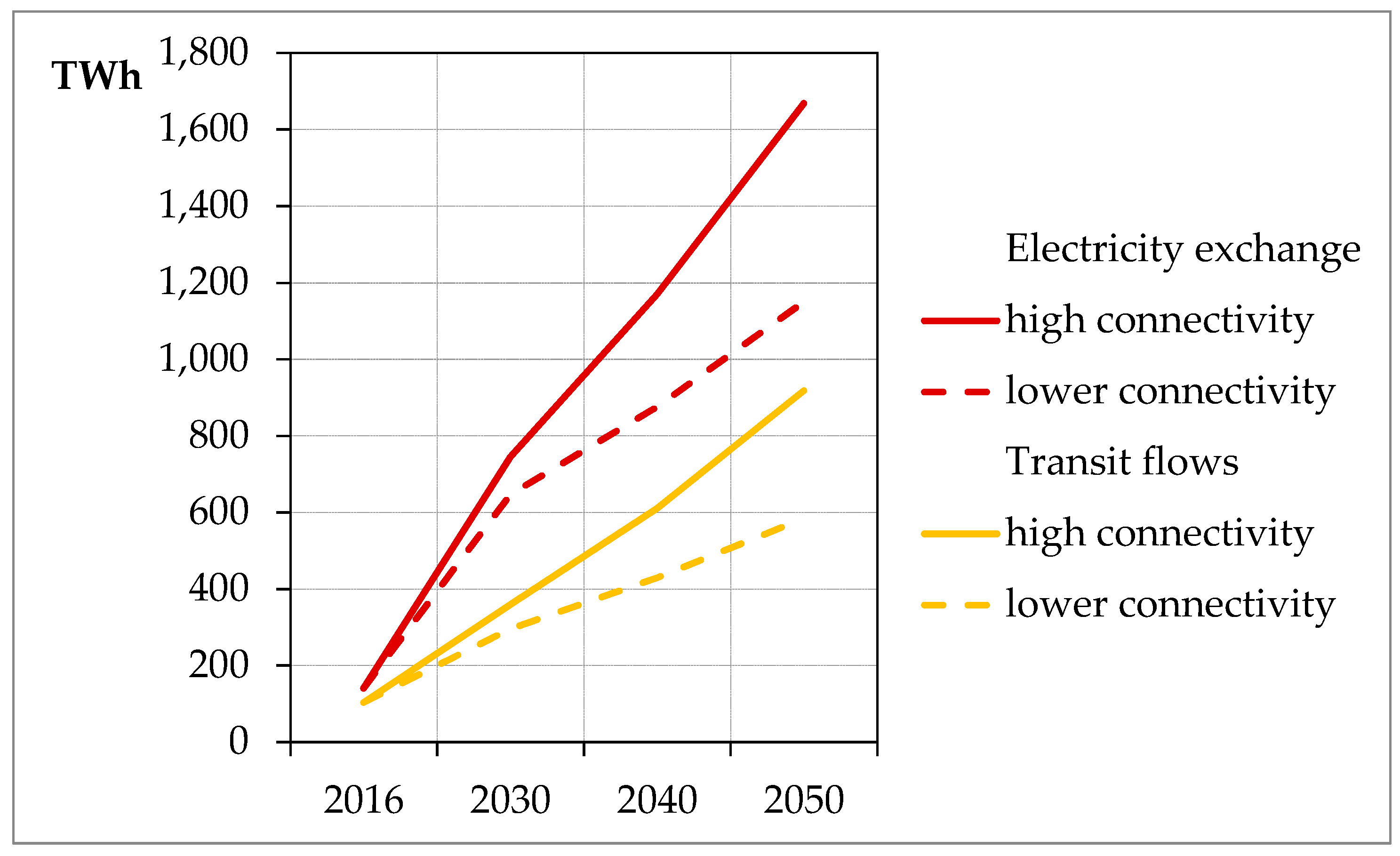
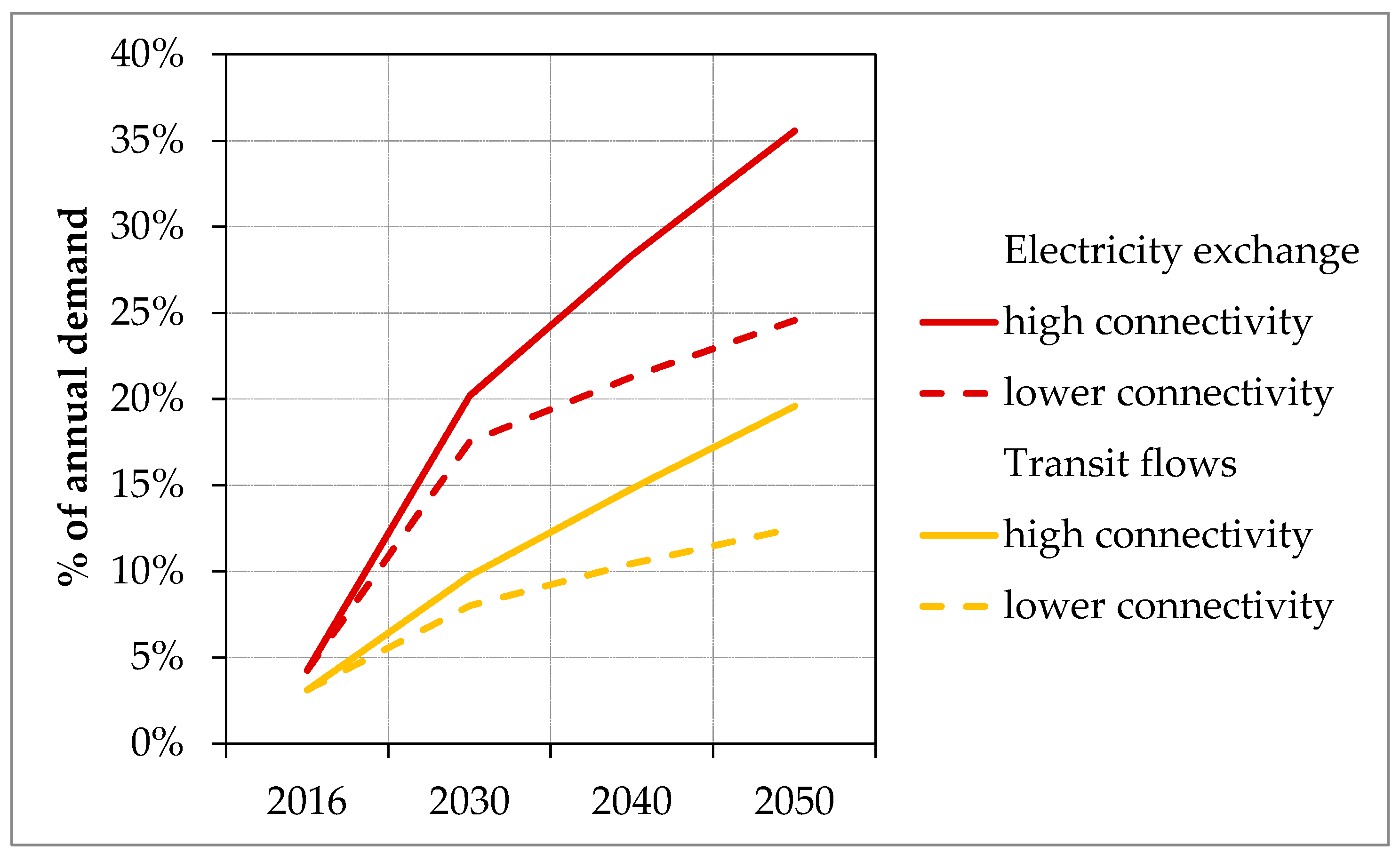
In the following, we compare our results for electricity exchange, electricity generation mix, CO2 emissions, and variable costs of electricity generation with the TYNDP 2018 “no grid” scenario.
Our analysis shows that a reduced expansion of interconnector capacities limits European electricity trading. It reduces electricity exchange between 13% in 2030 and 31% in 2050. In the TYNDP 2018 “no grid” scenario, this analysis is given as net annual balance per region and can, therefore, not be directly compared. However, the “no grid” view also comes to the conclusion that “the enhanced grid leads to a much greater level of power transfer between countries” (cf. [24] page 19).
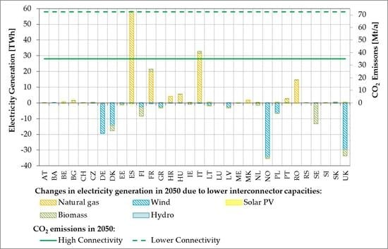
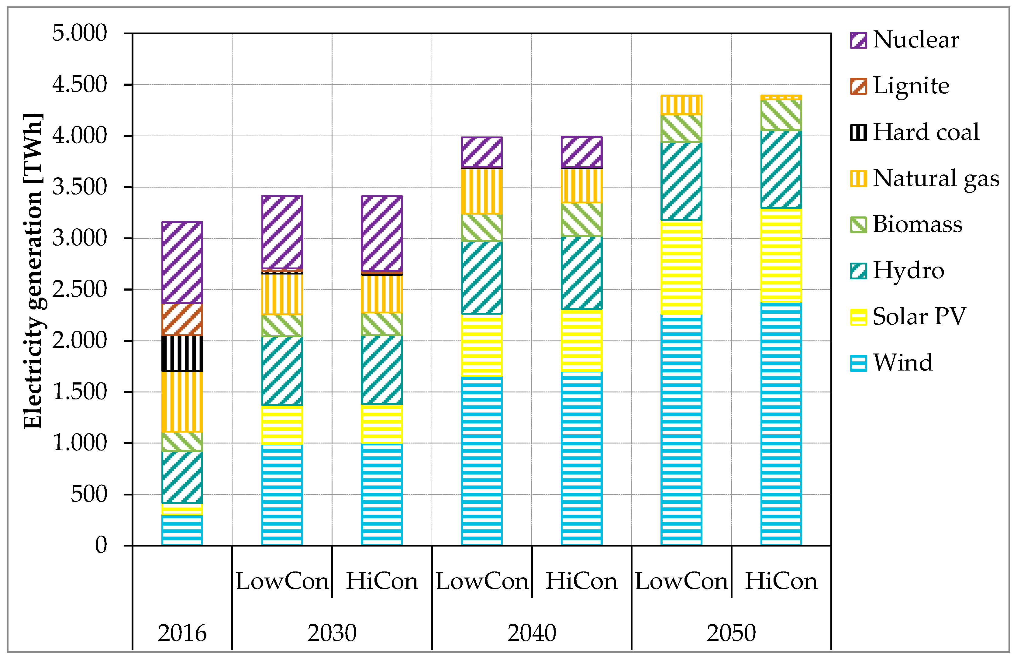
The electricity generation mix shifts toward technologies with higher generation costs due to the lower level of grid expansion. In our analysis, this effect is still relatively small in 2030, but increases by 2050, which is in line with the increasing RES-E expansion. This leads to an additional 47 TWh of RES-E curtailment in 2040 and 117 TWh in 2050. Gas-fired power plants compensate for the curtailed RES-E generation within Europe. In the TYNDP 2018 “no grid” analysis, the reduced grid expansion leads to approximately 156 TWh RES-E curtailment (cf. [24] page 22 f.). This stronger effect can be explained by the significantly stronger NTC reduction in the “no grid” scenario (cf. Table 5).
The changes in electricity generation lead to an increase in CO2 emissions. Due to the small changes in the generation mix in 2030, the effect on emissions is still relatively small in this year. In our analysis, in both 2040 and 2050, the additional emissions caused by the delayed expansion of the grid amount to approximately 37 million tons. For the year 2050, this would mean a doubling of CO2 emissions in the electricity sector. The stronger expansion of the grid can, thus, make a significant contribution toward reducing CO2 emissions. As a result of the greater grid reduction, the TYNDP 2018 “no grid” analysis also shows a stronger increase in CO2 emissions (+100 Mt) (cf. [24] page 23).
Due to the less efficient use of the European power plant fleet, the variable costs of electricity generation increase in the lower connectivity scenario. In our analysis, this increase amounts to 5% higher costs in 2030, 20% higher costs in 2040, and almost a doubling of costs in 2050. In addition to the overall stronger change in the electricity generation mix, this increase can be explained by two further elements. First, fuel and CO2 prices rise over the years, so that the additional use of natural gas power plants has a greater impact on electricity generation costs. Second, the higher share of renewable energy reduces generation costs, so that the relative changes in costs are more pronounced.
If there is no grid expansion, there would be higher electricity generation costs, but, at the same time, there would also be cost savings due to lower grid expansion costs. These grid-related cost savings were not taken into account in this analysis since our focus was on the effects of grid expansion in high RES-E scenarios. It was also assumed that there would be a delay in the expansion and that the grid would, therefore, be expanded at a later date. In the TYNDP 2018 “no grid” analysis, the reduced expansion of the grid resulted in electricity prices that would lead to consumer costs about three times the cost for the additional expansion of the grid, as calculated in the baseline scenario (cf. [24] page 17).

5. Conclusions

This paper concludes that the expansion of interconnector capacities can not only ensure a more efficient use of the European power plant fleet in the European internal market and associated cost savings but can also make an important contribution toward greenhouse neutrality. These effects increase over the years. On the one hand, this is due to the assumption that the absolute capacities of delayed projects will increase over the years with increasing grid expansion, which leads, over time, to a growing difference between the high connectivity and lower connectivity scenarios. On the other hand, due to the expansion of renewables, the spatial balance made possible by the European electricity grid becomes increasingly important. This observation is also shown in the TYNDP 2018 “no grid” analysis where the strongest effects are determined for the scenario with the highest RES-E share (cf. [24] page 17). This means that grid expansions that are planned today and that may be motivated to a large extent by cost savings achievable in the internal European market, are still relevant in a future high RES-E world with ambitious CO2 targets.
The identified effects of the delayed grid expansion can be interpreted as a conservative estimation. They would increase further with a lower level of alternative flexibilities such as batteries or power-to-gas. Compared to the assumptions in TYNDP 2018, a very strong expansion of interconnector capacities was assumed in the high connectivity scenario. As a result, the values of the lower connectivity scenario for 2030 and 2040 are approximately at the level of the TYNDP 2018 values. It can be assumed that, if the planned expansion of the grid was less pronounced, the restrictions on electricity exchange would become even more severe, and stronger effects would already become visible in the scenario year 2030.
Since both this paper as well as the TYNDP 2018 “no grid” analysis have shown the negative effects of a delayed expansion of interconnector capacities, the barriers for this expansion should be addressed. As described in Reference [20], the main obstacles are regulatory issues and acceptance problems. This is why a “simplified and standardized regulation” as well as a “strong and transparent consultation process in all stages” are proposed [20]. Bovet [43] additionally elaborates that the enforcement power of the two European legal instruments Projects of Common Interest and Ten-Year Network Development Plan should be strengthened, so that delays in the expansion of the European transmission grid can be addressed more effectively. In Reference [44], ENTSO-E and the Renewables Grid Initiative (RGI) describe how a lack of acceptance can be counteracted by "better projects." These "better projects" are characterized by “locally tailored, transparent, and participatory planning processes” [44].

Author Contributions

All authors contributed to the conceptualization of the research. D.R. took the lead in data curation, the analysis of the results, and in writing this paper. M.H. run the model software and wrote the model description in Section 2.1. R.M. developed the methodology to calculate the delay in NTC expansion and wrote the main part of Section 2.3. All authors have performed the validation of the results and have critically reviewed and edited the paper.

Funding

The German Federal Ministry for Economic Affairs and Energy, grant number 03ET4031A, funded this research.

Conflicts of Interest

The authors declare no conflict of interest. The funders had no role in the design of the study, in the collection, analyses, or interpretation of data, in the writing of the manuscript, or in the decision to publish the results.

Abbreviations

The following abbreviations are used in this paper.
aannum (per year)
ACERAgency for the Cooperation of Energy Regulators
bnbillion
CHPcombined heat and power plants
CO2carbon dioxide
ECEuropean Commission
ENTSO-EEuropean Network of Transmission System Operators for Electricity
EUEuropean Union
GAMSGeneral Algebraic Modeling System
GWgigawatt
hhour
HiConscenario high connectivity
KS 95Klimaschutzszenario 95
LowConscenario lower connectivity
Mtmegaton (1 million tons)
MWmegawatt
MWhmegawatt hour
NTCsnet transfer capacities
PCIProjects of Common Interest
PVphotovoltaic
PtGPower-to-Gas
RESrenewable energy source
RES-Eelectricity from a renewable energy source
RGIRenewables Grid Initiative
tton
TWhterawatt hour
TYNDPTen-Year Network Development Plan

Appendix A

Data Availability

The data sets as described in Table A1 are available in a country-specific resolution under the following link: https://zenodo.org/record/3257495.
Table A1. Fuel price (€/MWhth) and CO2 price (€/t CO2) scenario.
DataData TypeUnitInput/Output
DemandHourly profilesMWhInput
Variable RES-EHourly profilesMWhInput
Power plant fleetCapacitiesMWInput
NTCsCapacitiesMWInput
CO2 emissionsAnnual dataMtOutput
Variable costs of electricity generationAnnual dataM€Output
Variable costs of electricity generation per generation unitAnnual data€/MWhOutput
Electricity generationAnnual dataTWhOutput
Electricity exportAnnual dataTWhOutput
Electricity importAnnual dataTWhOutput
Transit flowsAnnual dataTWhOutput

Appendix B

Fuel and CO2 Prices

Table A2 shows the fuel and CO2 prices that were used for modeling. This data is based on Klimaschutzszenario 2050 [28].
Table A2. Fuel price (€/MWhth) and CO2 price (€/t CO2) scenario. Source: Reference [28].
203020402050
Oil (€/MWhth)597490
Gas (€/MWhth)344150
Coal (€/MWhth)121416
CO2 Prices (€/t CO2)87143200

Dimensioning of Batteries and Power-to-Gas Facilities

Batteries and PtG facilities are dimensioned per country and implemented as one large plant per country, since the national grid is not considered. Table A3 shows the main characteristics of storage technologies. The assumed parameters of the batteries concerning charge, discharge, and storage capacity as well as the ratio of battery capacity to installed PV capacity are based on the scenario framework from the German Network Development Plan 2030 (2019) [45]. Deriving the electrolyser capacity of power-to-gas, a ratio of 10% concerning the generation capacity of PV and wind is assumed. No restrictions are considered either for the re-conversion into electricity as well as for the storage capacity for synthetic gas. At country level, 100% of peak load is available for re-generation and 100% of the annual demand is available as storage capacity. Total efficiency of the batteries for the coupling of charging and discharging is 95% in all scenarios. For PtG flexibility, total efficiency increases over the scenario years from 34% to 38% (calculation based on Reference [46]).
Table A3. Characteristics of storage technologies. Source: References [45,46] and own assumptions.
TechnologiesCharge and Discharge CapacityStorage CapacityTotal Efficiency
Battery10% of installed PV capacity10% of installed PV capacity × 1 h95%
Power-to-Gas
(PtG)
Electrolyser capacity:
10% of PV and wind generation capacity
Reconversion into electricity:
100% of peak load
100% of total annual load2030: 34%
2040: 36%
2050: 38%

Derivation of Transit Flows

As described in the following equation, the annual transit flows per country ( T r a n s c ) are the sum of the hourly transit flows ( T r a n s t ). Therefore, the amount of imports and exports must be distinguished on an hourly basis. If, in the respective country, more imports (   I m p t ) than exports ( E x p t ) are made, the export quantities can be interpreted as transit flows. If the inverse case is given, import quantities must be used.
T r a n s t =   { E x p t   if     I m p t > E x p t I m p t if   I m p t < E x p t
T r a n s c = t = 1 8760 T r a n s t

Derivation of the Lower Connectivity Scenario

To derive our lower connectivity scenario, we adjusted the original NTC forecasts–serving as the idealized high connectivity scenario–for practical investment hurdles that may slow down the actual development of interconnection capacities. Below, we describe the underlying methodology of these adjustments.
Unfortunately, existing data even for the recent past is limited, and data bases do not allow for a quantification of how overall political ambitions for system integration or specific barriers may affect future NTC delays for each of the interconnectors. Instead, we focused on data about currently known investment delays and derive future numbers based on plausible assumptions.
A comparison of NTC forecasts from TYNDPs 2016 [37] and 2018 [5] reveals that expected NTC investments have undergone a significant downward adjustment. Figure A1 shows the interpolated forecasts of the accumulated NTC investments after 2015, according to TYNDP 2016 (Inv_2016) and TYNDP 2018 (Inv_2018) for the whole ENTSO-E area until 2030.
Figure A1. Accumulated NTC investments in the ENTSO-E area [5,37].
Energies 12 03098 g0a1
For the year 2020, the figure shows a relative reduction of accumulated investment numbers by 34%. In other words, between the two reported periods, total investment forecasts were corrected downward by one third of the original plans. Written formally, the relative adjustment of investments until 2020 ( Δ Inv 2020 ) is given by the equation below.
Δ Inv 2020 = Inv _ 2018 Inv _ 2016 Inv _ 2016   34 %
As the graphs show, investment forecasts in TYNDP 2018 catch up with the 2016 plans by 2026. We assume, however, that the main reason for this catch-up is that ENTSO-E calculations do not explicitly make assumptions about future investment delays. Instead of directly applying the specific numbers from the reports per year, we, therefore, decided to derive our own assumptions based on that we carry forward the relative adjustment for 2020 ( Δ Inv 2020 ) to later years. There are two main reasons for picking the 2020 value as a starting point. First, 2020 is the only year for which both reports provide forecasts. Hence, using 2020 avoids the uncertainty of data interpolation. Second, given that 2020 is relatively close to the TYNPD 2018 reporting period, we expect that most of the investment delays were already known when the forecasts were made and are, therefore, implicitly represented in the data.
Regarding the future development of investment delays, however, we have to rely on plausible assumptions. Drawing on the findings of ACER [21] and Roland Berger [19,36], we expect that permitting and regulatory issues are going to remain the dominant factor of investment delays and hurdles. Given that the lower connectivity scenario does not imply a strong political will to overcome administrative investment hurdles, the ambitious NTC investment plans will most likely be subject to additional delays. Hence, we assume that the spread between forecasted and actual investments will increase over time. We assume a regressive increase of the investment spread, which result in the downward-sloping curve for ΔInv shown in Figure 5 in Section 2.3.

Appendix C

For a better overview, the scenario presentations in Section 2.2.1 have been simplified. The detailed figures and data derivations are presented below.

Scenario Comparison-Electricity Demand

Figure A2 shows the development of electricity demand for selected scenarios. During the period up to 2050, most of the scenarios show a significant increase in demand, which can be attributed to an overcompensation of efficiency measures by an increase of new electricity consumers, such as electric mobility or heat pumps.
Figure A2. Annual electricity demand in EU28 countries. Sources: References [5,29,30,31,32].
Energies 12 03098 g0a2

Scenario Comparison-Renewable Generation Capacities

As shown in Figure A3, wind and solar capacities increase significantly in all scenarios. The ambitious scenario is located at the top and the unambitious scenario is located at the bottom of the scenario funnel. In the ambitious scenario, wind capacities are more than five times higher than in 2016, and solar capacities are more than six times higher. In the unambitious scenario, wind capacities more than double compared to 2016 and solar capacities almost triple compared to 2016.
While biomass capacities in most of the scenarios considered, double at most compared to the current level, in the scenario, 100% RES of the capacities undergo a six-fold increase. As described in Section 2.2.1, for the ambitious scenario, the values of the Big & Market scenario are used, as the increase of biomass capacities in the 100% RES scenario appears to be too strong, considering the competitive demand for land.
In most of the scenarios considered, hydro power capacities remain at about the current level or increase by half. In the 100% RES scenario, capacities more than double. In order not to overestimate the potential of hydro power, the values of the Big & Market scenario were also used here, since these are in the range of other scenarios. In addition, the assumed capacities were compared with the current level, and, for values that were lower, the current values were used. In the unambitious scenario, European hydro power generation capacities increase by approximately 10%.
Figure A3. Installed RES-E capacities in EU 28 countries. Sources: References [5,29,30,31,33].
Energies 12 03098 g0a3

Scenario Comparison-Conventional Generation Capacities

Figure A4 shows that, in most scenarios, natural gas capacities show a slight decline over the next few years, which is followed by an increase until 2050 to provide for sufficient secured capacity. As described in Section 2.2.1, natural gas capacities in e-Highway 2050 scenario 100% RES decline significantly by 2050. Since lower biomass and hydro power generation capacities were assumed (taken from the Big & Market scenario) for the ambitious scenario as compared with the 100% RES scenario, significantly higher values—from the Big & Market scenario—were used for natural gas capacities. Thus, in the ambitious scenario, natural gas capacities in 2050 are approximately 15% above today’s level. In the unambitious scenario, natural gas capacities increase by approximately 25% compared to today’s level.
In all scenarios, coal capacities decline significantly from the current level, even though levels reached in the scenario year 2050 differ significantly. While the ambitious scenario assumes a European-wide phase-out of coal by 2050, the unambitious scenario assumes that coal capacities will decline to approximately 35% by 2040 compared to 2016 and to approximately 33% by 2050.
The scenarios differ even more in the assumptions on nuclear power development. While some scenarios assume an increase in nuclear power, most scenarios assume at least a slight decline. In the unambitious scenario, nuclear power capacities decline to approximately 77% of today’s level. In the ambitious scenario, a European-wide nuclear phase-out is assumed.
Figure A4. Conventional generation capacities installed in EU 28 countries. Sources: References [5,29,30,31].
Energies 12 03098 g0a4

Appendix D

Installed Capacities and Generation Mix 2050 per Country

In this appendix, the installed capacities (cf. Table A4) and the generation mix (cf. Table A5 and Table A6) per country are presented for the scenario year 2050. As described in Section 2.2, the values for Germany are taken from Klimaschutzszenario 95 from Reference [28]. The capacities for the other countries are mainly based on scenario 100% RES from eHighway 2050 [29] (cf. Section 2.2 and Appendix C). Hydro power and biomass generation capacities increase very strongly in scenario 100% RES, which does not seem comprehensible from the perspective of natural restrictions respectively competing land use. Therefore, values of the eHighway 2050 Big & Market scenario [29] were used for these technologies. For hydro power generation capacities, it was further assumed that the installed capacities per country will not fall below the current level. In order to ensure that sufficient secure services are available, the size of natural gas capacities, which decrease significantly in the 100% RES scenario, was also taken from the eHighway 2050 scenario Big & Market. The derivation for power-to-gas and battery capacities is described in Appendix B.
Table A4. Installed capacities in GW, scenario year 2050. Source: References [28,29] and own assumptions.
Natural GasWind-OnWind-OffPV SolarBio-MassHydro-RunHydro-TurbinePumped StoragePower-to-GasBatteries
AT3.56.90.012.11.310.15.43.415.01.3
BA0.02.60.01.30.01.31.80.02.20.2
BE21.310.93.024.12.50.11.21.321.82.5
BG2.34.40.05.40.80.72.81.46.60.6
CH5.31.40.015.01.54.113.64.214.01.7
CZ0.510.20.013.01.00.61.11.212.61.3
DE3.998.327.298.60.44.36.315.779.112.3
DK0.518.725.62.03.00.00.00.07.60.2
EE0.58.10.00.80.30.00.00.52.30.1
ES29.369.40.0102.55.03.619.16.084.218.6
FI5.829.50.05.83.04.11.70.014.90.6
FR16.3124.20.0106.97.813.611.58.5130.514.0
GR3.025.90.015.11.00.43.31.612.42.7
HR1.86.30.03.80.00.52.50.34.60.4
HU4.04.90.014.01.30.30.30.010.21.6
IE1.813.60.03.80.30.40.50.57.90.3
IT46.841.30.0101.08.011.48.57.770.815.8
LT3.315.20.01.30.50.31.11.14.80.1
LU0.00.70.01.00.00.21.31.11.30.1
LV1.813.80.01.10.51.60.00.03.80.1
ME0.00.50.00.50.00.01.40.00.60.1
MK1.00.40.01.40.00.60.70.01.70.2
NL26.815.015.922.22.80.00.00.026.72.1
NO0.012.23.05.40.84.248.20.018.00.5
PL3.881.90.024.22.81.00.42.530.72.4
PT6.011.90.013.81.05.12.82.013.42.5
RO5.84.80.011.01.53.84.00.012.91.2
RS1.51.40.05.00.33.00.40.65.90.6
SE0.024.23.08.92.80.018.50.023.80.9
SI0.50.50.02.30.31.20.20.22.60.3
SK1.85.20.06.90.51.80.41.34.40.7
UK13.393.137.259.94.37.40.00.079.95.3
Sum211.4757.4114.9690.354.685.7159.060.9727.291.5
Table A5. Electricity generation in TWh, scenario year 2050 in the High Connectivity scenario. Source: own calculations.
Natural gasWind-OnshoreWind-OffshorePV SolarBio-MassHydro-runHydro-TurbinePumped StoragePower-to-GasBatteries
AT0.013.60.013.47.540.16.63.61.10.4
BA0.03.40.01.60.03.62.10.00.30.1
BE1.124.210.724.814.50.31.21.73.00.8
BG0.17.50.06.44.95.45.02.40.70.2
CH0.00.90.017.59.626.324.46.91.80.6
CZ0.120.40.013.36.01.01.31.31.50.4
DE10.6386.9163.7123.41.624.70.013.643.93.2
DK0.053.255.22.13.40.00.00.09.10.0
EE0.015.60.00.90.90.00.00.50.90.0
ES16.2145.00.0186.132.413.524.510.015.85.4
FI0.063.51.16.08.619.47.70.03.50.2
FR1.8272.73.6140.148.643.617.113.925.34.6
GR0.363.10.026.76.33.05.43.24.10.9
HR0.38.50.04.30.04.13.60.50.80.1
HU0.710.90.016.28.21.00.90.01.30.5
IE0.140.80.03.31.41.00.90.82.30.1
IT3.272.80.1158.051.542.815.814.511.95.2
LT0.031.80.01.32.40.92.11.21.90.0
LU0.01.30.01.00.00.82.41.00.10.0
LV0.125.00.01.21.84.30.00.01.40.0
ME0.00.70.00.60.00.21.60.00.10.0
MK0.20.40.01.70.01.82.90.00.10.1
NL0.047.859.720.615.50.10.00.06.30.6
NO0.048.612.85.31.018.7214.60.00.60.1
PL0.2128.90.023.614.54.80.72.79.70.7
PT1.031.60.125.46.413.63.53.42.40.8
RO0.87.50.012.49.814.66.00.01.10.4
RS0.01.70.05.71.78.91.91.10.40.2
SE0.049.612.58.814.00.076.30.01.50.2
SI0.00.60.02.71.64.40.30.30.30.1
SK0.27.00.07.43.35.40.82.31.10.3
UK0.0333.1143.752.821.522.30.00.027.41.9
Sum36.91918.4463.1914.4298.5330.7429.684.9181.528.1
Table A6. Electricity generation in TWh, scenario year 2050 in the Lower Connectivity scenario. Source: own calculations.
Natural GasWind-OnshoreWind-OffshorePV SolarBio-MassHydro-RunHydro-TurbinePumped StoragePower-to-GasBatteries
AT0.013.60.013.47.640.16.64.01.40.4
BA0.03.40.01.60.03.62.10.00.20.0
BE1.924.210.724.814.40.31.21.94.00.8
BG1.57.50.06.45.15.45.01.90.40.2
CH0.00.90.017.59.926.324.45.91.00.5
CZ0.120.40.013.36.31.01.31.41.90.4
DE10.0380.2151.5123.41.624.70.014.457.03.2
DK0.051.642.42.10.10.00.00.08.90.0
EE0.014.90.00.90.30.00.00.51.10.0
ES74.0144.30.0186.132.713.524.58.79.05.0
FI0.061.10.96.02.719.47.70.04.10.2
FR21.7272.33.5140.150.043.617.112.117.44.0
GR0.360.50.026.75.73.05.43.04.40.9
HR4.38.50.04.30.04.13.60.40.50.1
HU6.110.90.016.28.41.00.90.00.80.4
IE0.640.10.03.31.21.00.90.82.20.1
IT34.772.40.1158.052.742.815.812.47.94.6
LT0.630.30.01.32.00.92.11.42.50.1
LU0.01.30.01.00.00.82.41.10.10.0
LV0.022.40.01.21.24.30.00.02.00.0
ME0.00.70.00.60.00.21.60.00.10.0
MK2.00.40.01.70.01.82.90.00.10.1
NL0.447.859.620.614.10.10.00.07.40.7
NO0.026.90.05.30.018.7214.60.00.00.0
PL0.8122.30.023.614.44.80.73.012.00.7
PT3.631.50.125.46.513.63.53.11.70.7
RO15.27.50.012.310.114.66.00.00.70.3
RS0.01.70.05.71.78.91.90.90.30.2
SE0.049.512.48.80.90.076.30.02.00.1
SI0.00.60.02.71.74.40.30.30.10.1
SK0.67.00.07.43.35.40.81.80.70.2
UK0.7329.1118.052.817.422.30.00.030.91.9
Sum179.01865.4399.1914.4272.0330.7429.678.9182.526.0

References

  1. United Nations (UN). Status 7. d Paris Agreement. Available online: https://treaties.un.org/Pages/ViewDetails.aspx?src=TREATY&mtdsg_no=XXVII-7-d&Section=27&clang=_en#EndDec (accessed on 17 May 2019).
  2. United Nations Framework Convention on Climate Change (UNFCCC). Paris Agreement; UNFCCC: Bonn, Germany, 2015. [Google Scholar]
  3. European Commission (EC). 2050 Long-Term Strategy. 2018. Available online: https://ec.europa.eu/clima/policies/strategies/2050_en (accessed on 17 May 2019).
  4. European Commission (EC). In-Depth Analysis in support of the commission communication com (2018) 773. A Clean Planet for All. A European Long-Term Strategic Vision for a Prosperous, Modern, Competitive and Climate Neutral Economy, Brussels. 2018. Available online: https://ec.europa.eu/clima/sites/clima/files/docs/pages/com_2018_733_analysis_in_support_en_0.pdf (accessed on 17 May 2019).
  5. ENTSO-E. TYNDP 2018 Scenario Report. Data Set, Brussels. 2018. Available online: https://tyndp.entsoe.eu/maps-data/ (accessed on 8 February 2019).
  6. Andersky, T.; Sanchis, G.; Betraoui, B. e-HIGHWAY 2050—Modular Development Plan of the Pan-European Transmission System 2050. Deliverable 2.1. Available online: https://www.dena.de/fileadmin/dena/Dokumente/Pdf/9013_MOB_Brochure_ehighway2050_englisch.pdf (accessed on 3 September 2018).
  7. Tafarte, P.; Eichhorn, M.; Thrän, D. Capacity Expansion Pathways for a Wind and Solar Based Power Supply and the Impact of Advanced Technology—A Case Study for Germany. Energies 2019, 12, 324. [Google Scholar] [CrossRef]
  8. Schlachtberger, D.P.; Brown, T.; Schramm, S.; Greiner, M. The benefits of cooperation in a highly renewable European electricity network. Energy 2017, 134, 469–481. [Google Scholar] [CrossRef] [Green Version]
  9. Kost, C.; Längle, S. The Spatial Dimension of the Energy Transition: European Renewable Energy Sources. Local Resources and International Exchange; The European Dimension of Germany’s Energy Transition. Opportunities and Conflicts. Available online: https://www.springer.com/de/book/9783030033736#otherversion=9783030033743 (accessed on 29 May 2019).
  10. Hagspiel, S.; Jägemann, C.; Lindenberger, D.; Brown, T.; Cherevatskiy, S.; Tröster, E. Cost-Optimal Power System Extension under Flow-based Market Coupling; EWI Working Paper No 13/09. 2013. Available online: https://www.ewi.uni-koeln.de/cms/wp-content/uploads/2015/12/EWI_WP_13_09.pdf (accessed on 4 June 2019).
  11. European Commission (EC). Energy Union and Climate: Making Energy more Secure, Affordable and Sustainable. Available online: https://ec.europa.eu/commission/priorities/energy-union-and-climate_en (accessed on 3 September 2018).
  12. European Commission (EC). EU Budget: Commission Proposes Increased Funding to Invest in Connecting Europeans with High-Performance Infrastructure, Brussels. 2018. Available online: http://europa.eu/rapid/press-release_IP-18-4029_en.htm (accessed on 17 May 2019).
  13. European Commission (EC). Progress Towards Completing the Internal Energy Market; EC: Brussels, Belgium, 2014. [Google Scholar]
  14. Schmid, E.; Knopf, B. Quantifying the long-term economic benefits of European electricity system integration. Energy Policy 2015, 87, 260–269. [Google Scholar] [CrossRef] [Green Version]
  15. Bauknecht, D.; Heinemann, C.; Koch, M.; Ritter, D.; Harthan, R.; Sachs, A.; Vogel, M.; Tröster, E.; Langanke, S. Systematischer Vergleich von Flexibilitäts- und Speicheroptionen im deutschen Stromsystem zur Integration von erneuerbaren Energien und Analyse entsprechender Rahmenbedingungen, Freiburg, Darmstadt. 2016. Available online: https://www.oeko.de/fileadmin/oekodoc/Systematischer_Vergleich_Flexibilitaetsoptionen.pdf (accessed on 19 January 2017).
  16. DNV GL.; Imperial College London; NERA Economic Consulting. Integration of Renewable Energy in Europe; Final Report; EC: Brussels, Belgium, 2014. [Google Scholar]
  17. Child, M.; Kemfert, C.; Bogdanov, D.; Breyer, C. Flexible electricity generation, grid exchange and storage for the transition to a 100% renewable energy system in Europe. Renew. Energy 2019, 139, 80–101. [Google Scholar] [CrossRef]
  18. Fuersch, M.; Hagspiel, S.; Jägemann, C.; Nagl, S.; Lindenberger, D.; Tröster, E. The role of grid extensions in a cost-efficient transformation of the European electricity system until 2050. Appl. Energy 2013, 104, 642–652. [Google Scholar] [CrossRef] [Green Version]
  19. Roland Berger. The Structuring and Financing of Energy Infrastructure Projects, Financing Gaps and Recommendations Regarding the New TEN-E Financial Instrument; Final Report to the European Commission; EC: Brussels, Belgium, 2011. [Google Scholar]
  20. Battaglini, A.; Komendantova, N.; Brtnik, P.; Patt, A. Perception of barriers for expansion of electricity grids in the European Union. Energy Policy 2012, 47, 254–259. [Google Scholar] [CrossRef]
  21. Agency for the Cooperation of Energy Regulators (ACER). Consolidated Report on the Progess of Electricity and Gas Projects of Common Interest for the Year 2015; ACER: Ljubljana, Slovenia, 2016. [Google Scholar]
  22. Rodríguez, R.A.; Becker, S.; Andresen, G.B.; Heide, D.; Greiner, M. Transmission needs across a fully renewable European power system. Renew. Energy 2014, 63, 467–476. [Google Scholar] [CrossRef] [Green Version]
  23. Becker, S.; Rodriguez, R.A.; Andresen, G.B.; Schramm, S.; Greiner, M. Transmission grid extensions during the build-up of a fully renewable pan-European electricity supply. Energy 2014, 64, 404–418. [Google Scholar] [CrossRef]
  24. ENTSO-E. European Power System 2040 Completing the Map. The Ten-Year Network Development Plan (TYNDP) 2018 System Needs Analysis, Brussels. 2018. Available online: https://docstore.entsoe.eu/Documents/TYNDP%20documents/TYNDP2018/european_power_system_2040.pdf (accessed on 24 May 2019).
  25. Koch, M.; Bauknecht, D.; Heinemann, C.; Ritter, D.; Vogel, M.; Tröster, E. Modellgestützte Bewertung von Netzausbau im europäischen Netzverbund und Flexibilitätsoptionen im deutschen Stromsystem im Zeitraum 2020–2050. Zeitschrift für Energiewirtschaft 2015, 39, 1–17. [Google Scholar] [CrossRef]
  26. Koch, M.; Flachsbarth, F.; Bauknecht, D.; Heinemann, C.; Ritter, D.; Winger, C.; Timpe, C.; Gandor, M.; Klingenberg, T.; Tröschel, M. Dispatch of Flexibility Options, Grid Infrastructure and Integration of Renewable Energies Within a Decentralized Electricity System. In Advances in Energy System Optimization: Proceedings of the first International Symposium on Energy System Optimization; Bertsch, V., Fichtner, W., Heuveline, V., Leibfried, T., Eds.; Birkhäuser: Cham, Switzerland, 2017; pp. 67–86. ISBN 978-3-319-51794-0. [Google Scholar]
  27. Bundesministerium für Umwelt, Naturschutz und nukleare Sicherheit (BMU). Projektionsbericht 2019 für Deutschland gemäß Verordnung (EU) Nr. 525/2013, 2019. Available online: https://cdr.eionet.europa.eu/de/eu/mmr/art04-13-14_lcds_pams_projections/projections/envxnw7wq/ (accessed on 25 June 2019).
  28. Repenning, J.; Hermann, H.; Emele, L.; Jörß, W.; Blanck, R.; Loreck, C.; Böttcher, H.; Ludig, S.; Dehoust, G.; Matthes, F.C.; et al. Klimaschutzszenario 2050. 2. Modellierungsrunde, Berlin. 2015. Available online: https://www.oeko.de/oekodoc/2451/2015-608-de.pdf (accessed on 15 May 2017).
  29. Andersky, T.; Sanchis, G.; Betraoui, B. e-Highway 2050—Database Per Country; Excel-Sheet; EC: Brussels, Belgium, 2016. [Google Scholar]
  30. Matthes, F.C.; Blanck, R.; Greiner, B.; Zimmer, D.W. The Vision Scenario for the European Union. 2017 Update for the EU-28; Greens/EFA Group in the European Parliament: Brussels, Belgium, 2018. [Google Scholar]
  31. European Commission (EC). EU Reference Scenario 2016. Energy, Transport and GHG Emissions—Trends to 2050; EC: Brussels, Belgium, 2016. [Google Scholar]
  32. Eurostat. Supply, Transformation and Consumption of Electricity—Annual Data. nrg 105a. Available online: http://appsso.eurostat.ec.europa.eu/nui/show.do?dataset=nrg_105a&lang=en (accessed on 20 May 2019).
  33. Eurostat. Infrastructure—Electricity—Annual Data. nrg113a. Available online: http://appsso.eurostat.ec.europa.eu/nui/show.do?dataset=nrg_113a (accessed on 20 May 2019).
  34. Gesetz über die friedliche Verwendung der Kernenergie und den Schutz gegen ihre Gefahren; Atomgesetz; German Federal Ministry of Justice and for Consumer Protection: Berlin, Germany, 2018.
  35. ENTSO-E. Transparency Platform. Available online: https://transparency.entsoe.eu/ (accessed on 29 May 2019).
  36. Roland Berger. Permitting Procedures for Energy Infrastructure Projects in the EU: Evaluation and Legal Recommendations; Final Report to the European Commission; EC: Brussels, Belgium, 2011. [Google Scholar]
  37. ENTSO-E. TYNDP 2016. Market Modelling Data. 2015. Available online: https://tyndp.entsoe.eu/maps-data/ (accessed on 3 September 2018).
  38. Agency for the Cooperation of Energy Regulators (ACER). Recommendation of the ACER No 02/2016 on the Common Capacity Calculation and Redispatching and Countertrading Cost Sharing Methodologies; ACER: Ljubljana, Slovenia, 2016. [Google Scholar]
  39. European Commission (EC). Communication from the Commission to the European Parliament, the Council, the European Economic and Social Committee and the Committee of the Regions: Communication on Strengthening Europe’s Energy Networks; EC: Brussels, Belgium, 2017. [Google Scholar]
  40. Sandbag. EU ETS Dashboard. Available online: http://sandbag-climate.github.io/EU_ETS_Dashboard.html (accessed on 29 May 2019).
  41. United Nations Framework Convention on Climate Change (UNFCCC). Member States’ CRF Submissions to UNFCCC. 2018. Available online: https://unfccc.int/process/transparency-and-reporting/reporting-and-review-under-the-convention/greenhouse-gas-inventories-annex-i-parties/national-inventory-submissions-2018 (accessed on 29 May 2019).
  42. Bossavy, A.; Bossmann, T.; Fournié, L.; Humberset, L.; Khallouf, P. METIS Studies. Study S1: Optimal Flexibility Portfolios for a High-RES 2050 Scenario. 2018. Available online: https://publications.europa.eu/en/publication-detail/-/publication/f26e4340-67fd-11e9-9f05-01aa75ed71a1/language-en/format-PDF/source-96288622 (accessed on 4 June 2019).
  43. Bovet, J. The Electricity Transmission Line Planning Process at European Level. Legal Framework and Need for Reforms; The European Dimension of Germany’s Energy Transition. Opportunities and Conflicts. Available online: https://www.springer.com/de/book/9783030033736#otherversion=9783030033743 (accessed on 29 May 2019).
  44. ENTSO-E.; Renewables Grid Initiative (RGI). Working Paper May 2019: Value of Timely Implementation of “Better Projects”. 2019. Available online: https://docstore.entsoe.eu/Documents/Publications/Position%20papers%20and%20reports/20190517_RGI_ENTSOE_working_paper_better_projects.pdf (accessed on 24 May 2019).
  45. Bundesnetzagentur (BNetzA). Genehmigung des Szenariorahmens 2019–2030; BNetzA: Bonn, Germany, 2018. [Google Scholar]
  46. Agora Verkehrswende; Agora Energiewende. Die zukünftigen Kosten strombasierter synthetischer Brennstoffe, Berlin. 2018. Available online: https://www.agora-energiewende.de/fileadmin2/Projekte/2017/SynKost_2050/Agora_SynCost-Studie_WEB.pdf (accessed on 23 May 2018).
Figure 1. Comparison of annual electricity demand in EU 28 countries based on References [5,29,30,31,32].
Energies 12 03098 g001
Figure 2. Comparison of RES-E capacities installed in EU28 countries based on References [5,29,30,31,33].
Energies 12 03098 g002
Figure 3. Comparison of conventional generation capacities installed in EU 28 countries based on References [5,29,30,31].
Energies 12 03098 g003
Figure 4. Electricity demand and installed capacities in Germany. Source: References [28,35].
Energies 12 03098 g004
Figure 5. Development of relative NTC investment adjustment (own calculations and assumptions based on References [5,37]).
Energies 12 03098 g005
Figure 6. Development of total NTC in the ENTSO-E area [5,29]. *Increase of the NTCs due to a higher NTC to thermal grid capacity ratio: 2016: Ø 31% [38], 2025: min. 70% [39].
Energies 12 03098 g006
Figure 7. NTCs between the countries considered and their sum of export capacities in the high connectivity scenario for the year 2050. Source: Reference [29].
Energies 12 03098 g007
Figure 8. Electricity exchange and transit flows.
Energies 12 03098 g008
Figure 9. Electricity exchange and transit flows in relation to electricity demand.
Energies 12 03098 g009
Figure 10. Electricity generation in the ENTSO-E area. Source: 2016 [32,35].
Energies 12 03098 g010
Figure 11. Change in electricity generation in 2050 due to lower connectivity levels.
Energies 12 03098 g011
Figure 12. Development of CO2 emissions in the ENTSO-E area. Source: 2016 [40,41].
Energies 12 03098 g012
Table 1. RES-E share and curtailment in the ENTSO-E area.
203020402050
LowConHiConLowConHiConLowConHiCon
RES-E share of demand (%)62%63%81%84%96%99%
RES-E curtailment (TWh)1325811238121
Table 2. CO2 emissions in the ENTSO-E area in 2016 and in the scenario years (absolute (Mt/a), effect of lower connectivity (Mt/a), and reduction compared to 2016 (%)). Source: 2016 [40,41].
2016203020402050
20161020
LowCon (Mt/a) 31717772
HiCon (Mt/a) 29914035
LowCon-HiCon (Mt/a) 18.536.937.4
LowCon vs. 2016 (%) 69%83%93%
HiCon vs. 2016 (%) 71%86%97%
Table 3. Variable costs of electricity generation in the ENTSO-E area.
(bn €/a)203020402050
LowCon77.471.842.6
HiCon73.959.722.2
LowCon-HiCon3.512.120.5
Table 4. Variable costs of electricity generation per MWh electricity produced in the ENTSO-E area.
(€/MWh)203020402050
LowCon20.917.49.1
HiCon20.014.54.7
LowCon-HiCon0.93.04.4
Table 5. Comparison of RES-E share in electricity demand and assumptions for NTC reduction in the TYNDP 2018 and this study. Source: Reference [24] and own calculation.
YearRES-E ShareNTC Reduction in the “No Grid” and Lower Connectivity Scenarios, Respectively
TYNDP 2018204064%–80%40%–47%
This study203063%27%
204084%32%
205099%37%

