Small Signal Stability with the Householder Method in Power Systems
by
 , , and
Asghar Sabati
1,*, 
Ramazan Bayindir
2,
Sanjeevikumar Padmanaban
3,* ,
,
Eklas Hossain
4 and
Mehmet Rida Tur
5 1
Energy R&D Center, EUROPOWER, PC 06980 Ankara, Turkey
2
Department of Electrical & Electronics Engineering, Gazi University, PC 06500 Ankara, Turkey
3
Department of Energy Technology, Aalborg University, 6700 Esbjerg, Denmark
4
Oregon Renewable Energy Center (OREC), Department of Electrical Engineering and Renewable Energy, Oregon Tech, Klamath Falls, OR 97601, USA
5
Department of Electrical & Energy Engineering, Batman University, PC 72500 TBMYO, Batman, Turkey
*
Authors to whom correspondence should be addressed.
Energies 2019, 12(18), 3412; https://doi.org/10.3390/en12183412
Submission received: 1 August 2019
/
Revised: 27 August 2019
/
Accepted: 30 August 2019
/
Published: 4 September 2019
(This article belongs to the Special Issue Advanced Signal Processing Techniques Applied to Power Systems Control and Analysis)
Abstract
:Voltage collapse in power systems is still considered the greatest threat, especially for the transmission system. This is directly related to the quality of the power, which is characterized by the loss of a stable operating point and the deterioration of voltage levels in the electrical center of the region exposed to voltage collapse. Numerous solution methods have been investigated for this undesirable degradation. This paper focuses on the steady state/dynamic stability subcategory and techniques that can be used to analyze and control the dynamic stability of a power system, especially following a minor disturbance. In particular, the failure of one generator among the network with a large number of synchronous generators will affect other synchronous generators. This will become a major problem and it will be difficult to find or resolve the fault in the network due to there being too many variables, consequently affecting the stability of the entire system. Since the solution of large matrices can be completed more easily in this complex system using the Householder method, which is a small signal stability analysis method that is suggested in the thesis, the detection of error and troubleshooting can be performed in a shorter period of time. In this paper, examples of different rotor angle deviations of synchronous generators were made by simulating rotor angle stability deviations up to five degrees, allowing the system to operate stably, and concluding that the system remains constant.
1. Introduction
Developing technology, ever-growing urbanization and environmental conditions have forced energy systems to work close to the stability limit. This has increased the importance given to the subject of voltage stability and it has become much more important. The stability of a power system is the ability to keep the amplitudes of continuous or transient load bus bars within certain limits. In addition, voltage stability is the ability of these power systems to return to their former stable state when confronted with a disturbing effect and to retain the voltage in all bus bars within a certain level. One of the criteria for qualifying a system as a stable system is if the power given to a bus bar increases numerically, the amplitude of the voltage in that bus bar increases and this process proceeds similarly for all other bus bars in the system. If the reactive power given to that bus bar is increased in any of the bus bars in the system, and the voltage amplitude does not increase, it can then be said that there is voltage instability in this system [1]. Also, if the V-Q sensitivity for each bus bar is directly proportional or positive, the system is stable in terms of voltage. Thus, if the V-Q sensitivity is negative for at least one bus bar, the system voltage is unstable. Failure of power systems to reach a voltage stability state is referred to as a “voltage failure”, which occurs in the event of overload, failure, or insufficient reactive power. In recent years, the voltage stability problem called voltage collapse has been experienced quite a lot. This has led to an increase in voltage stability studies [2,3]. In some studies, solutions are made by providing a methodology aimed at maintaining frequency stability by taking into account the latency associated with the frequency measurement process, while acquiring virtually equal inertia limitations from virtual operational generators [4]. Voltage stability and voltage instability are described depending on the size of static faults that may occur [5]. The oscillations in power systems raise voltage-related problems along with a small signal stability problem, which is one of the most important factors that limit power transmission capacity and jeopardize safe operation [6,7]. Analytical solutions and mathematical models were used to analyze the effect of stochastic continuous disturbances on the power system small signal stability [8,9].
This study aims to estimate the modal characteristics of the system including modal frequency, damping and shape. Most of the signal processing algorithms described in this section are the basis of developing several software tools. The majority of these tools are used to perform an engineering analysis on the grid in an offline or post-degradation environment [10]. Online real-time software tools and applications have recently been developed [11] and will continue to be the focus of research for the power system community. Voltage stability is sometimes referred to as load balancing [12]. The terms voltage instability and voltage collapse are often used interchangeably. Voltage instability is a dynamic process involving voltage dynamics, as opposed to rotor angle (synchronous) stability. Voltage collapse is defined as a process in which voltage instability in a significant portion of the system leads to a very low voltage profile. The voltage instability limit is not directly connected to the maximum power transmission limit of the grid [5,11,12]. Generally, local modes are in the range of 1–2 Hz, while in-field modes can range from 0.2 to 1.0 Hz [13]. Typically, in-field modes cause a little more trouble. Consistent with the dynamic system of a power system, it can be linearized at an operating point of the power system [10,11]. The proposed method offers an advantage for the difficulty of stability analysis of nonlinear systems. In addition, it is impossible to practically analyze very large powerful complex systems. The systems examined in this article are not actually of a linear nature. Since the deviations occurring at the equilibrium are small (small signal), they can be approximated to the linear system. Therefore, instead of analyzing the nonlinear system, we can analyze the system approximated to being linear, which is easier.
Stability in a power system means that the system normally has the desired parameters. In other words, it can be defined as the ability of the system to return to its nominal state in a short period in case of a failure. In some studies, a small signal and a large signal stability analysis were performed using the Lyapunov linearization method. A combined stability criterion was then proposed to predict small and large signal stability problems [14,15,16]. In a power system, when the system is in a stable state, there is equilibrium between the incoming mechanical momentum and the outgoing electrical momentum. This equilibrium causes the velocity to remain constant. When short-circuit faults are also included, the equilibrium may be explained in terms of static stability. If an error occurs between power systems, the balance between the incoming mechanical momentum and the outgoing electrical momentum is relatively eliminated. According to the law of motion of rotating objects, the synchronous machine rotor will have a positive or negative speed, so it will rotate at high or low speed compared to other generators. This uncoordinated rotation will alter the stability of the system by changing the rotor angle. Furthermore, this problem is solved by using an approach based on the largest Lyapunov base for online transient rotor angle stability assessment using data from large area measurement systems only [17,18].
Thanks to the studies conducted on maintaining small signal stability, a few advantages in large power systems will be addressed. One of the benefits of small signal stability is that each synchronous generator present in the system can be linearized around the operating point. However, differential equations need to be solved systematically in transient stability, where the differential equations that dominate the pre-fault system, the during-fault power system, and the equations that dominate the post-fault system must be solved. Furthermore, if the protection relays do not work in the system during this time, the system will lose its synchronized state. It is not possible to find differential equations, even when solved in a systematic manner, that determine the cleaning time and security index in the relays after the fault. In order to find the critical time, the system needs to be simulated several times in all error-occurring situations, which will result in a great loss of time, and the fact that the system inspects its behavior for errors will reduce the time to intervene and cause even more time loss. However, the time spent in inspection of small signal stability is between 10 and 20 s. In the case of small signal stability, the stability of the system can be determined very easily through the master data, and only the positive or negative data will be sufficient to examine the stability of the system, without the need to inspect the data even after the calculations.
This article provides an overview of the challenges applied to the prediction of time-synchronized data of more successful analysis techniques of electromechanical mode. The theoretical basis, applications and performance characteristics of these methods are explained. When inter-zone modes are studied in a power system, several generators fluctuate in the opposite direction compared to other generators due to other failures. This is caused by a connection of two groups of generators over a weak line. The frequency of these fluctuations is between 0.2 and 1 Hz. Regional and comprehensive modes are today’s most modern modes and are studied in stability studies of power systems. As modern power systems are directly connected to each other, the connection lines are often outdated and due to their high costs, the renewal of the lines is avoided. Despite the construction of new power plants, inter-regional fluctuations often occur because these power plants are connected to power systems through weak lines. Many PSS studies today are focused on power systems. The PSS system should not use local signals. However, it can use signals from other regions as input signals. In this case, too, a delay may occur when the signal is sent from other regions, which may impair the small signal stability. When there are multiple synchronous machines, the variable parameters will increase, and the mathematical analysis of the system will become more difficult. It is very difficult to find the determinant of a large matrix. Therefore, the straightforward method can only be discussed theoretically, but it does not have much use in practice. In the determination of the main quantities by means of numerical methods such as the square method, inverse square method and the Arnold method, the largest main amount is obtained in terms of absolute magnitude. Consequently, different measures should be taken to find other main quantities. For this reason, the method of similar transformations is one of the practical methods. In the Gionesis Rotation method, which is based on orthogonal similarities, only one element in the given matrix is reset at each stage after transformation. Because of repeated transformations, the given matrix is orthogonally homologized to an upper triangle or Hasenberg Matrix. Thus, the given matrix can be decomposed as QR (Q, an orthogonal matrix; R, an upper triangular matrix). The main advantage of the Householder method presented in this article is that each column of the given matrix is transformed into the column of an upper-triangular matrix at each transformation stage. This method is important when compared particularly to the Gionesis method because, in the Gionesis method, for the transformation of an (n × n) matrix to an upper-triangular matrix, a conversion (matrix multiplication) operation must be performed n (n – 1/2) times. However, the conversion operation must be performed, at most, n times in the Householder method. In numerical terms of the data, the number of computational operations is important, because rounded errors can accumulate due to the large number of operations and ultimately have an impact on the result. In particular, when the actual specific quantities are close to zero, these rounded errors may not be able to determine the sign of that main quantity. Therefore, the method presented is of great importance—both in terms of the number of computational operations and in terms of obtaining all the main quantities—and has undeniable superiority over similar methods.
2. Materials and Methods
2.1. Mathematical Model of Small Signal Problems
Synchronizing and Damping Momentums: When a short circuit occurs, the momentum of a synchronous machine is divided into two components. In order for a power system to exist, both components must be present. The lack of synchronizing momentums in a power system leads to instability that is dependent on the rotor angle and is not of the fluctuation type. The lack of damping momentums causes fluctuation instability. If one generator runs temporarily faster than the other does, the angular position of the rotor will increase in connection to that of the slow machine. The resulting angular difference transfers a portion of the load from the slow machine to the fast machine based on the theoretically known power angle relationship. This tends to reduce the speed difference and therefore the angular aperture. Further angular aperture may lead to a decrease in power transfer, leading to greater instability [19].
- : Synchronous momentum;
- : Coefficient of synchronous momentum;
- : Damping momentum (has the same phase as ∆ω);
- TD: Coefficient of damping momentum.
This involves the protection of predetermined bus voltages by a power system to reach a stable state after a fault or short circuit occurs [20]. Therefore, the main reason for the instability in voltage is that the power system fails to provide reactive power. In other words, because the reactive power is directly proportional to the voltage, the electric power system has not been able to provide the reactive power required in its network well [1,21]. If for some reason (such as the input or output of a large production unit) the voltage drops in a part of the network and other generators or systems that compensate for the reaction power return to the current system, the voltage returns to its normal state [22]. Otherwise, the voltage drop will reach an unacceptable value and cause a power failure in another part of the power system network, which is called a voltage collapse [3,23,24].
2.2. Definition of the Single Machine Infinite Bus (SMBI)
The infinite bus is a source of voltage with constant voltage and frequency. Due to the infinite bus, the generator dynamics will not change EB voltage and frequency. In terms of small signal stability, both space- and block-type display methods are used to represent the small signal. In topics related to stability, the classical model is used to model the generator [25]. In this model shown as Figure 1, the generator is modeled as a voltage source connected to the reactance; however, all resistances in the generator or synchronous machine are ignored.
Calculation of complex and active forces in the network using flow equations:
‘p’ is the power of air distance. p does not indicate the voltage of the terminal generator. However, since the stator resistance is ignored while the generator model is conventionally shown, P is also shown as the power of the terminal generator so that other analyzes can be performed.
Another important point is that the air distance momentum is equal to the air distance power. The air distance momentum is as in Equation (6).
One of the most important equations related to rotor angle stability is the air distance momentum equation, and the other is the fluctuation equation (motion equation) [26].
2.2.1. Linearization Model of Equations in Small Signal Stability (Sinδ, Cosδ)
In order to achieve small signal stability, the air distance momentum must be converted to a linear equation around the working point δ = δ0. To achieve this goal, first the sine in the air distance equation is linearized, so that the entire air distance equation can then be linearized [27]. Sinδ, Cosδ linearization around δ = δ0 equilibrium: a small deviation indicated by Δδ can be linearized as in the following equations:
δ0 = rotor angle at equilibrium
Based on Sinδ, Cosδ equations and trigonometric relations:
The most important result obtained from the above equations is Δ δ = 1.
Considering the above equations, when Te becomes linear at the working point δ = δ0, it becomes as follows in Equation (11).
- Tm: Mechanical momentum;
- Ks: Synchronous momentum coefficient.
Small signal stability can be analyzed by obtaining the master data. The representation of the linearized equation in the space matrix is as in Equation (15).
- Ks: Synchronous momentum coefficient;
- KD = Stabilizer momentum coefficient (stabilizer);
- H = Coefficient of inertia.
Equations belonging to the system are determined by considering the input and output of the system; then the system’s main data is found using these equations and the system’s small signal stability can be examined [28].
At this stage, in order to find the main data, the Equation (20) must be equal to zero [29].
The general representation of second-order equations will be as in Equation (21): ζ = Stability ratio
The equations belonging to ωn ve ζ can also be found using the equations in Equations (20) and (21):
- As Ks increases; the natural frequency increases, the stability rate decreases.
- The stability ratio increases as kD increases.
- As H increases, both the ωn rate and the stability rate ζ decrease [30].
2.2.2. Control of Dynamic Systems
In a dynamic system, xi variables of the system affect each other. Each variable of the system is a function in terms of time. The aim of the analysis of dynamic systems is to examine the future behavior of the system. These behaviors include the determination of critical points and limit circles, examination of system stability, chelation, and chaos control.
If there is no change in rotor angle and speed, i.e., Δω (0) =Δ (0) = 0, and no change in mechanical momentum, the system will remain stable as per ΔTm (t) =0. For example, ΔTmt = 0, Δω0 = 0, Δδ0 = 5o ≈ 0.0875 Rad; in this case, KD = 10, KS = 0.757, H = 3.5, ω0 = 377.0δ
The real portions of both quantities are negative, so the system is stable shown as Figure 2.
If the damper coefficient becomes 0 (KD = 0) in the above example, the response and master data of the system will be as follows in Figure 3.
The real part of both master data is equal to zero. Therefore, the system does not go towards zero (stability) or infinity (instability). Instead, it continues its own fluctuation state. In another case shown as Figure 4, if the damping coefficient always changes as KD = −10, the master data and the response diagram of the system change as follows:
The response of the system, as can be seen, is positive for both quantities. Therefore, the system is unstable, as the diagram shows, and the fluctuation ranges of the system increase as time goes on. When the excitation system is taken into account, the matrix of the system is per Equation (24).
The dynamics of a synchronous generator with PSS will be as in Equation (25) below.
![Energies 12 03412 i001]()

2.2.3. Multi-Machine Synchronous Systems
As mentioned in the previous sections, the master data of the mode matrix plays an important role in system stability. The real parts of these quantities show exponential changes and the space matrix parts show fluctuation changes in sine. If the real part is negative, the exponential part of the response will tend towards zero. As a result, the fluctuating part will also be influenced by this and tend towards zero [31].
However, if some of the master data contains non-negative real parts, the responses will not tend to zero over time. However, it either will tend towards infinity with growing fluctuations (if the master data is positive) or will continue with the previous fluctuation (if the master data is negative). Thus, even a small amount of chaos will be enough to disrupt the balance of the system. As it can be understood from these explanations, it is sufficient to know the position of the master data on the complex surface in the analysis of linear systems, but it is also sufficient to know the sign in the real part of the master data. In the following sections, methods of finding master data in large systems will be examined. If the dynamic system of each machine is as shown in Equation (27) below [32].
Thus, the master data of the matrix of the above situation will determine the state of the system. In general, this matrix is a large sparse matrix and it is difficult to find its main data [33].
2.2.4. Householder Method Small Signal Stability
Many methods are based on orthogonal similarity. If two matrices are homologous, then the QR matrices present in the Homologous Transformations and a QR Algorithm will be as in Equation (32), since they have the same principal amounts as well as the same polynomials. For the separation of orthogonal and an upper triangular matrix, the transposed ‘p’ is obtained by multiplying the air distance by the force. The main advantage is obtained by transforming the resulting matrix.
If U is a unit vector, the Householder Matrix Hu is defined as follows per Equation (37):
If A, n × n is a matrix, then B, the transformation of A through the Householder transformation, will be as in Equation (39).
If the generated Hu matrix is indicated by :
Thus, the matrix A is decomposed into QR. If the expression is zero, U will not be able to be defined. Therefore, the matrix A cannot be homologous to an upper-triangular matrix orthogonally by the QR algorithm. In this case, the matrix in discussion can be orthogonally made homologous to the previous Hessenberg Matrix. As a result, instead of the master data of matrix A, the master data of the Hessenberg Matrix is found. There are two famous assumptions on this topic.
3. Results
Considering a 20 bus bar grid model where current is injected by four generators, the Ad matrix having the damping coefficient difference will be a 24 × 24 cross-block matrix, as shown in Figure 5.
It is possible to find the master data of the system matrix via the following program. In addition, the system’s response to any change in parameters can be plotted and the output current of all generators can be monitored after each failure. In addition, the range of change of parameters can be determined upon system stability and the most appropriate mode can be selected shown as Table 1. The objective is to estimate and 5°, 3° deviations in the first and third synchronous generators, respectively. The location of the 24th master data on a complex surface is shown in Figure 6.
The real part of the master data is completely negative, so the system is stable, and each minor fault returns to a stable state after a short time. The following Figure 7 shows how the condition variables of each generator, variation diagrams and other variables are changed by the deviation of the rotor angle by 5 degrees in the first generator and by 3 degrees in the third generator.
In general, the total active electrical power supplied by the generators should always be equal to the active power consumed by the loads, which also includes the losses in the system. A failure in the system can disrupt this balance, causing the rotors of the generators to accelerate or decelerate. If one generator temporarily runs faster than the other does, the angular position of the rotor will increase in connection to that of the slower machine shown as Figure 8. Variation diagram of four generators when .
As can be seen in variation diagram of four generators when , the system has remained stable as the real part of the master data is negative. The minimum changes of rotor angle and speed of some generators did not affect the stability of the system and the system regained its stability after these minimum failures.
Evaluation of the Proposed Solution Method
The analysis of linear systems is much simpler than that of nonlinear systems. As can be seen in this article, the position of the matrix state on the complex surface for the main quantities was found because of the analysis of linear systems. Furthermore, the sign of the real portions of the matrix state of the main quantities (positive or negative) showed the stability of the system. If these real parts are negative, the system is stable and small deviations will not disrupt this stability, but after a short time, the system will regain its equilibrium. Any changes in the parameters of the generator and network will affect the elements of the matrix state; therefore, the location of the main quantities on the complex surface will vary, because of which the stability of the system will be affected. In this thesis, we attempted to examine how changes in the damping coefficient affect the main quantities of the state matrix, and the diagrams of the changes in the real parts of each main quantity were drawn against the changes in the [−200,200] range of the damping coefficient (KD). The system is unstable in KDs where the real part of at least one main quantity is negative. Therefore, the above diagrams show the effect of the damping coefficient on system stability. In addition, these diagrams can be drawn based on changes of other parameters and system stability can be examined. As a result, the stability of large systems in the small signal depends only on finding the main quantities of a very large matrix. In fact, finding the main quantities is possible by finding the roots of a polynomial equation derived from the determinant, det(A-λI). In other words, only n-1 steps are necessary for the conversion of the given matrix to an upper-triangular matrix. In the first stage, the elements below the element (1,1) are reset; in the second stage, the ones under element (2, 2) are reset; and in the final stage, only the ones under element (n, n − 1) are reset.
4. Conclusions
This article demonstrates the formation of voltage stability in a system using conventional and small signal stability methods used to differentiate voltage stability. According to the literature, the non-linear system of the Household Method has been found to provide a linearization around the working point provided that the signal that changes the working point is small. Thus, it has been proved that easier linear systems can be analyzed instead of analysis of demanding nonlinear systems. However, it is not easy to obtain the Lyapunov Function to study the stability of a fixed point. This is because there is no general method for finding this function. The complex ambiance will be compared to non-linear functions with thousands of variables by using the concepts of coordinate functions. It has been shown that it is almost impossible to examine ultra-large systems with hundreds and thousands of variables without linearizing them. The only practical way of examining large systems is small signal analysis, since it can be linearized. The stability analysis of these systems is related to finding the master data of the mode matrix. Whether the real parts of these values are negative or positive determines whether the system is stable. Although it is highly challenging to find the master data of such a large matrix, it can be facilitated by making it linear so that the application capability of computer simulation can be improved.
The methods of finding the master data of large matrices are generally designed on homologous transformations (especially Householder transformations), because the successive transformations of the householder will result in many zeros in the columns of the matrix. The QR decomposition is made with the matrix obtained through the multiplication of the orthogonal matrix by the upper triangular matrix. The matrix obtained using the QR algorithm is then multiplied by the upper-triangular matrix (if this matrix does not exist, by the upper Hessenberg Matrix) and made homologous. Homologous transformations and degrees of the master data are retained so that, since the master data of the triangular matrix, the elements on the diagonal, the master data of the resulting matrix emerges from the triangular matrix. The QR algorithm can also generate the master data matrix (Modal Matrix). It is also designed to find the zero of functions in some other algorithms. These methods consider a particular polynomial as a function and try to find the zeros of the function by methods such as the Newton–Raphson Method. Other methods that are better suited than the Newton–Raphson Method are also used in finding the zero of different functions. Another method to find the master data is to use random algorithms. To achieve this goal, finding zeros is considered as minimizing, and then using complementary algorithms, such as genetic algorithms, solutions are provided for these issues. As a result, the most efficient method of finding main data in order to perform small signal stability analysis in large power systems is the Householder Method.
Author Contributions
Conceptualization, A.S. and M.R.T.; Methodology, A.S.; Software, E.H.; Validation, R.B., S.P. and A.S; Formal Analysis, M.R.T.; Investigation, A.S.; Resources, A.S.; Data Curation, M.R.T and E.H.; Writing-Original Draft Preparation, M.R.T.; Writing-Review & Editing, M.R.T.; Visualization, R.B.; Supervision, R.B and S.P.
Funding
This research received no external funding.
Conflicts of Interest
The authors declare no conflict of interest
References
- Pierre, D.A.; Trudnowski, D.J.; Hauer, J.F. Identifying reduced-order models for large nonlinear systems with arbitrary initial conditions and multiple outputs using Prony signal analysis. In Proceedings of the 1990 American Control Conference, San Diego, CA, USA, 23–25 May 1990; Volume 1, pp. 149–154. [Google Scholar]
- Thompson, S.C.; Ahmed, A.U.; Proakis, J.G.; Zeidler, J.R.; Geile, M.J. Constant Envelope OFDM Abbrev. IEEE MILCOM. Military Commun. Conf. 2008, 56, 1300–1312. [Google Scholar]
- Lindell, G.; Sundberg, C.E.W. An Upper Bound under bir error probability of combine convolution coding and continuous phase modulation. IEEE Trans. Inform. Theory 1988, 1, 1263–1269. [Google Scholar] [CrossRef]
- Khan, S.; Bletterie, B.; Anta, A.; Gawlik, W. On Small Signal Frequency Stability under Virtual Inertia and the Role of PLLs. Energies 2018, 11, 2372. [Google Scholar] [CrossRef]
- Taylor, C.W. Power Systems Voltage Stability; Electric Power Research Institute, McGraw Hill: New York, NY, USA, 1994. [Google Scholar]
- Rajaraman, R.; Dobson, I.; Sarlashkar, J.V. Analytical modeling of thyristor-controlled series capacitors for SSR studies. IEEE Trans. Power Syst. 1996, 11, 15–32. [Google Scholar]
- Martins, N. Retuning Stabilizers for the North-South Brazilian Interconnection. In Proceedings of the 1999 IEEE Power Engineering Society Summer Meeting, Edmonton, AB, Canada, 18–22 July 1999; Volume 1, pp. 58–67. [Google Scholar]
- Lui, W. Research on a Small Signal Stability Region Boundary Model of the Interconnected Power System with Large-Scale Wind Power. Energies 2015, 8, 2312–2336. [Google Scholar] [CrossRef] [Green Version]
- Xu, Y. Stochastic Small Signal Stability of a Power System with Uncertainties. Energies 2018, 11, 2980. [Google Scholar] [CrossRef]
- Parashar, M.; Mo, J. Real Time Dynamics Monitoring System (RTDMSTM): Phasor applications for the control room. In Proceedings of the 42nd Annual Hawaii International Conference on System Sciences (HICSS-42), Big Island, HI, USA, 5–8 January 2009; Volume 1, pp. 5–8. [Google Scholar]
- Abe, S.; Isono, A. Determination of power system voltage stabilitiy. Electr. Engeland Jpn. 1983, 103, 3–13. [Google Scholar]
- Hauer, J.F. Application of Prony analysis to the determination of modal content and equivalent models for measured power system response. IEEE Trans. Power Syst. 1991, 6, 1062–1068. [Google Scholar] [CrossRef]
- Bourgin, F.; Testud, G.; Heilbronn, B.; Verseille, J. Present Practics and Trends on the French Power System to Prevent Voltage Collapse. IEEE Trans 1993, 8, 3–13. [Google Scholar]
- Willems, J.L. Stability Theory of Dynamical Systems; Wiley Interscience Division: London/Nelson, UK, 1970. [Google Scholar]
- Chi-Tsong, T.C. Linear Systems Theory and Design; Academic Press: New York, NY, USA; London, UK, 1984. [Google Scholar]
- Che, Y.; Xu, J.; Shi, K.; Liu, H.; Chen, W.; Yu, D. Stability Analysis of Aircraft Power Systems Based on a Unified Large Signal Model. Energies 2017, 10, 1739. [Google Scholar] [CrossRef]
- Dher, D.K.; Doolla, S.; Bandyopadhyay, S. Electrical Power and Energy Systems Effect of placement of droop based generators in distribution network on small signal stability margin and network loss. Int. J. Electr. Power Energy Syst. 2017, 88, 108–118. [Google Scholar] [CrossRef]
- Haung, D.; Chen, Q.; Ma, S.; Zhang, Y.; Chen, S. Wide-Area Measurement—Based Model-Free Approach for Online Power System Transient Stability Assessment. Energies 2018, 11, 958. [Google Scholar] [CrossRef]
- Berrou, C.; Glavieux, A.; Thitimajshima, P. Near Shannon-Limit error correcting coding and decoding: Turbo codes. Proc. ICC93 1993, 3, 1064–1070. [Google Scholar]
- Bezerra, H.L.; Martins, N. Eigenvalue methods for calculating dominant poles of a transfer function and their applications in small-signal stability. Appl. Math. Comput. 2019, 347, 113–121. [Google Scholar] [CrossRef]
- Anderson, J.B.; Aulin, T. Digital Phase Modulation; Electronics & Electrical Engineering, Applications of Communications Theory; Springer Science & Business Media: New York, NY, USA, 1986. [Google Scholar]
- Khodadad, A.; Divshali, P.H.; Nazari, M.H.; Hosseinian, S.H. Small-signal stability improvement of an islanded micro grid with electronically-interfaced distributed energy resources in the presence of parametric uncertainties. Electr. Power Syst. Res. 2018, 160, 151–162. [Google Scholar] [CrossRef]
- Bourgin, F.; Testud, G.; Heilbronn, B.; Verseille, J. Present practices and trends on the French power system to prevent voltage collapse. IEEE Trans. PWRS 1993, 8, 3–13. [Google Scholar] [CrossRef]
- Hill, D.J. Nonlinear dynamic load models with recovery for voltage studies. IEEE Trans. PWRS 1993, 8, 1. [Google Scholar] [CrossRef]
- IEEE Special Stability Control Working Group. Static VAR Compensator Models for Power Flow and Daynamic Performance Simulation. IEEE Trans. PWRS 1994, 9, 1. [Google Scholar]
- Robak, S.; Gryszpanowicz, K. Rotor angle small signal stability assessment in transmission network expansion planning. Electr. Power Syst. Res. 2015, 128, 144–150. [Google Scholar] [CrossRef]
- IEEE Task Force. Proposed Terms and Defin. for Power System Stability. IEEE Trans. 1982, 7, 1894–1898. [Google Scholar]
- Lu, X.; Xiang, W.; Lin, W.; Wen, J. Small-signal modeling of MMC based DC grid and analysis of the impact of DC reactors on the small-signal stability. Electr. Power Energy Syst. 2018, 101, 25–37. [Google Scholar] [CrossRef]
- Xie, R.; Kamwa, D.; Rimorov, D.; Moeini, A. Fundamental study of common mode small-signal frequency oscillations in power systems. Electr. Power Energy Syst. 2019, 106, 201–209. [Google Scholar] [CrossRef]
- Weiyu, W. Virtual Synchronous Generator Strategy for VSC-MTDC and the Probabilistic Small Signal Analysis. IFAC-Pap. Line 2017, 50, 5424–5429. [Google Scholar] [CrossRef]
- Sadhana, G.S. Small Signal Stability Analysis of Grid Connected Renewable Energy Resources with the Effect of Uncertain Wind Power Penetration. Energy Procedia 2017, 117, 769–776. [Google Scholar] [CrossRef]
- Guo, C.; Zheng, A.; Yin, Z.; Zhao, C. Small-signal stability of hybrid multi-terminal HVDC system. Electr. Power Energy Syst. 2019, 109, 434–443. [Google Scholar] [CrossRef]
- Yang, W.; Norrlund, P.; Chung, C.Y.; Yang, J.; Ludin, U. Eigen-analysis of hydraulic-mechanical-electrical coupling mechanism for small signal stability of hydropower plant. Renew. Energy 2018, 115, 1014–1025. [Google Scholar] [CrossRef]
Figure 1.
Classic model diagram in a Single Machine Infinite Bus (SMIB) system.

Figure 2.
Diagram of the simulation of the rotor angle and speed changes up to 10 s.
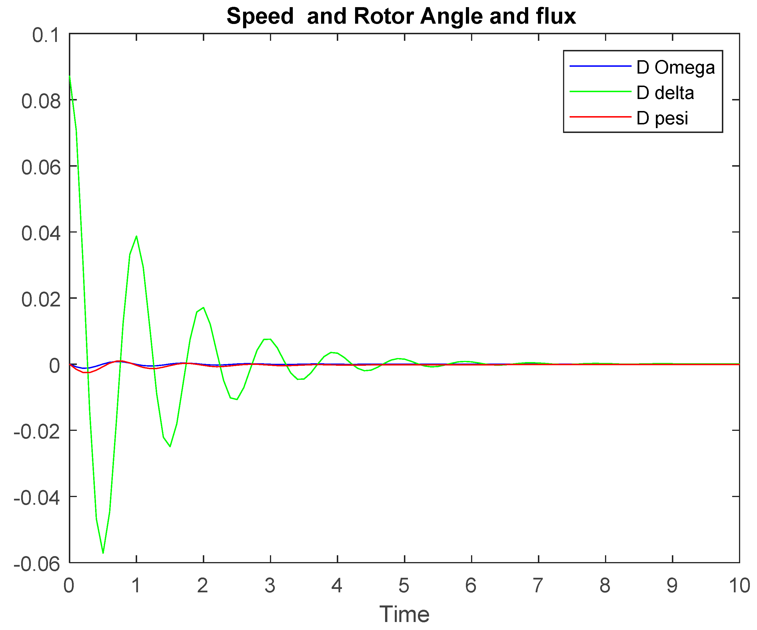
Figure 3.
Response diagram of the system fluctuating between stability and instability.
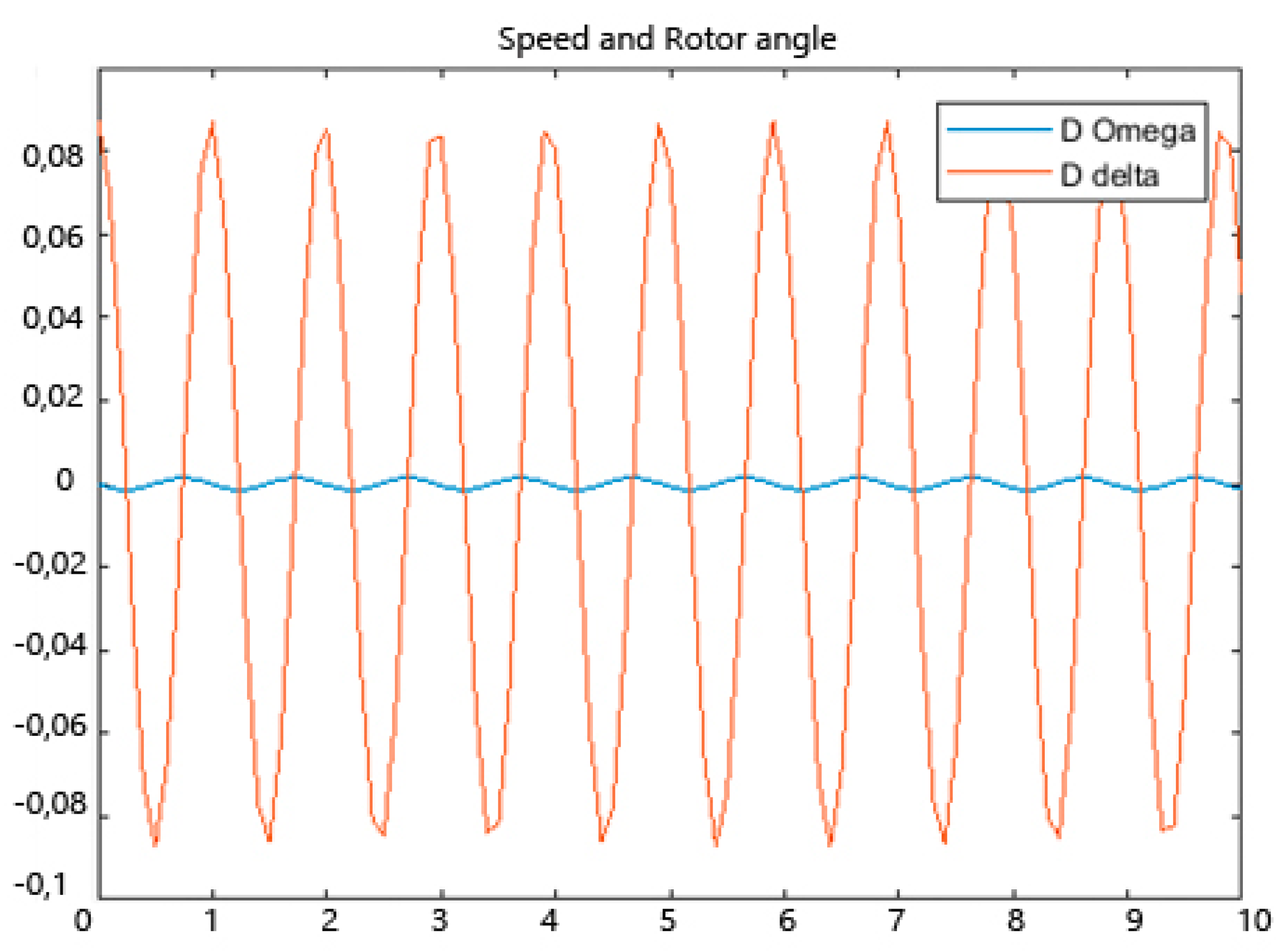
Figure 4.
The system response in which there is a linear relationship between instability and time.

Figure 5.
20-bus bar power system.
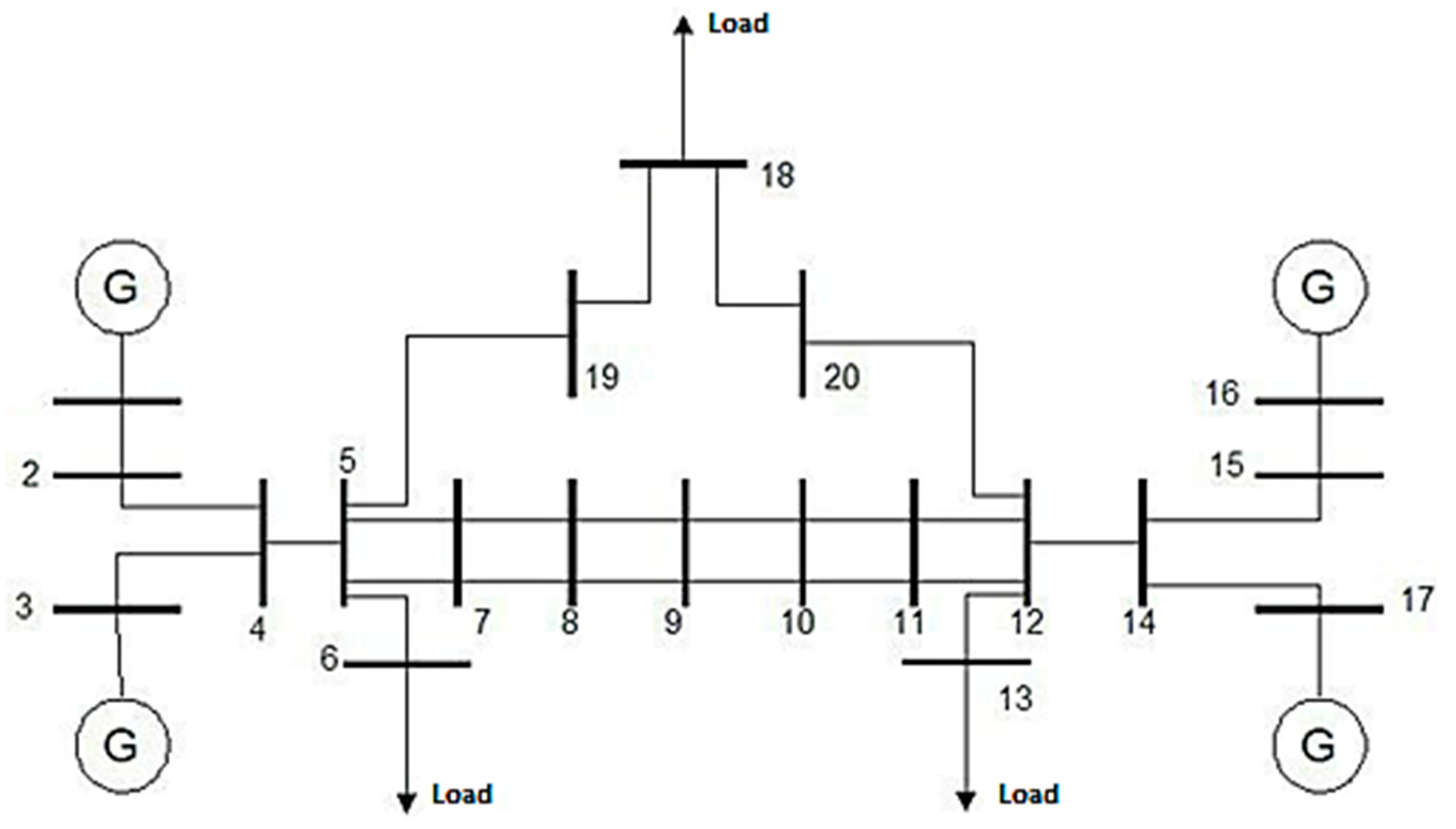
Figure 6.
Location of the 24th master data on a complex surface.
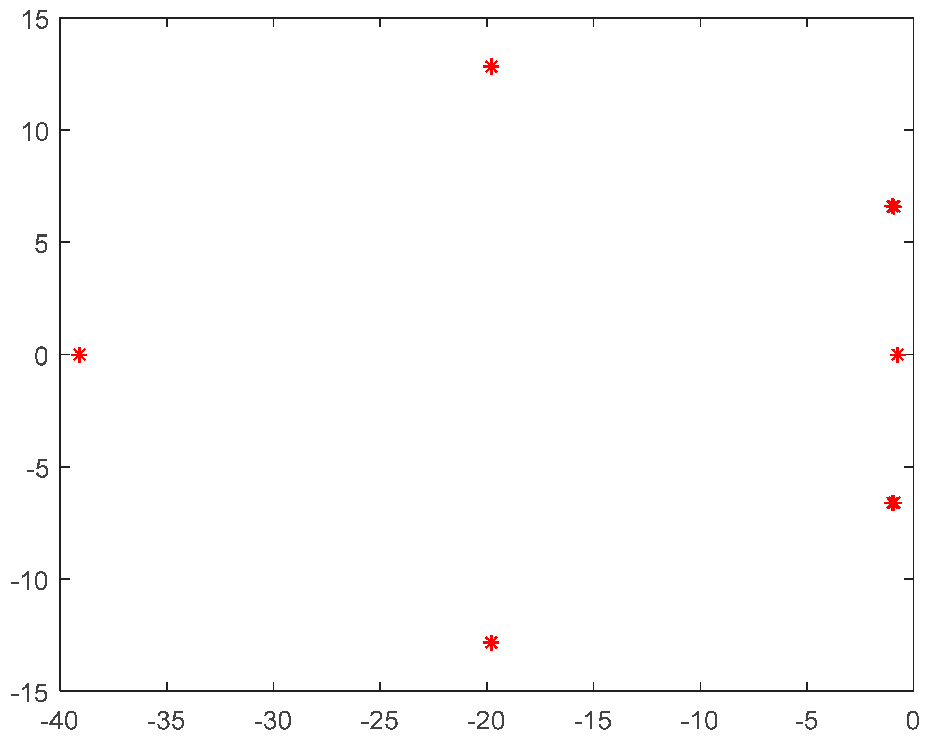
Figure 7.
Shows the damping momentum stability diagram of the generators in the power system.
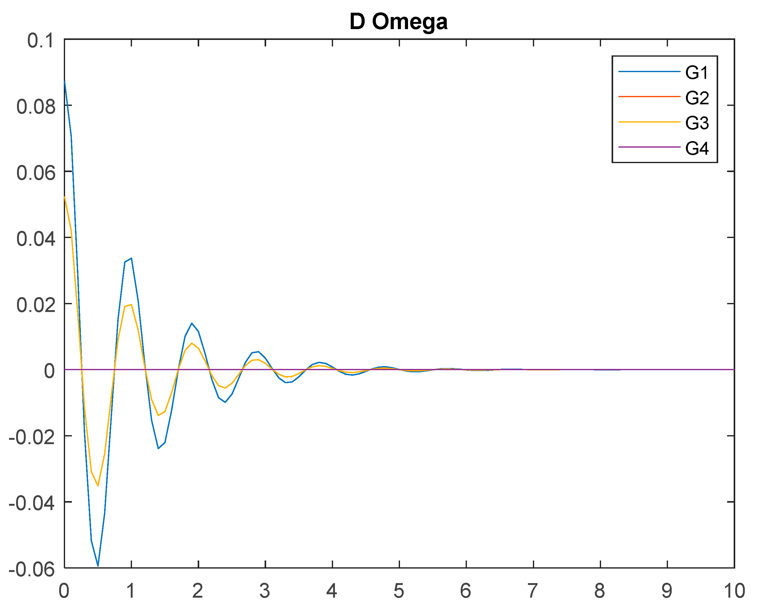
Figure 8.
Variations diagram of generators in a power system.


Table 1.
The data of special matrix values.
| No. | Real Part | Imaginary Part |
|---|---|---|
| Landa1 | −39.0967416 | +0.000000000000000i |
| Landa2 | −1.00550148 | +6.607284341444071i |
| Landa3 | −1.00550148 | −6.607284341444071i |
| Landa4 | −0.738513482 | +0.000000000000000i |
| Landa5 | −19.79697098 | +12.822376834424755i |
| Landa6 | −19.79697098 | −12.822376834424755i |
| Landa7 | −39.0967416 | +0.000000000000000i |
| Landa8 | −1.00550148 | +6.607284341444071i |
| Landa9 | −1.00550148 | −6.607284341444071i |
| Landa10 | −0.738513482 | +0.000000000000000i |
| Landa11 | −19.79697098 | +12.822376834424755i |
| Landa12 | −19.79697098 | −12.822376834424755i |
| Landa13 | −39.0967416 | +0.000000000000000i |
| Landa14 | −1.00550148 | +6.607284341444071i |
| Landa15 | −1.00550148 | −6.607284341444071i |
| Landa16 | −0.738513482 | +0.000000000000000i |
| Landa17 | −19.79697098 | +12.822376834424755i |
| Landa18 | −19.79697098 | −12.822376834424755i |
| Landa19 | −39.0967416 | +0.000000000000000i |
| Landa20 | −1.00550148 | +6.607284341444071i |
| Landa21 | −1.00550148 | −6.607284341444071i |
| Landa22 | −0.738513482 | +0.000000000000000i |
| Landa23 | −19.79697098 | +12.822376834424755i |
| Landa24 | −19.79697098 | −12.822376834424755i |
© 2019 by the authors. Licensee MDPI, Basel, Switzerland. This article is an open access article distributed under the terms and conditions of the Creative Commons Attribution (CC BY) license (http://creativecommons.org/licenses/by/4.0/).
Share and Cite
MDPI and ACS Style
Sabati, A.; Bayindir, R.; Padmanaban, S.; Hossain, E.; Rida Tur, M. Small Signal Stability with the Householder Method in Power Systems. Energies 2019, 12, 3412. https://doi.org/10.3390/en12183412
AMA Style
Sabati A, Bayindir R, Padmanaban S, Hossain E, Rida Tur M. Small Signal Stability with the Householder Method in Power Systems. Energies. 2019; 12(18):3412. https://doi.org/10.3390/en12183412
Chicago/Turabian StyleSabati, Asghar, Ramazan Bayindir, Sanjeevikumar Padmanaban, Eklas Hossain, and Mehmet Rida Tur. 2019. "Small Signal Stability with the Householder Method in Power Systems" Energies 12, no. 18: 3412. https://doi.org/10.3390/en12183412
Note that from the first issue of 2016, this journal uses article numbers instead of page numbers. See further details here.