Determination of Transient Fluid Temperature and Thermal Stresses in Pressure Thick-Walled Elements Using a New Design Thermometer

Abstract

In both conventional and nuclear power plants, the high thermal load of thick-walled elements occurs during start-up and shutdown. Therefore, thermal stresses should be determined on-line during plant start-up to avoid shortening the lifetime of critical pressure elements. It is necessary to know the fluid temperature and heat transfer coefficient on the internal surface of the elements, which vary over time to determine transient temperature distribution and thermal stresses in boilers critical pressure elements. For this reason, accurate measurement of transient fluid temperature is very significant, and the correct determination of transient thermal stresses depends to a large extent on it. However, thermometers used in power plants are not able to measure the transient fluid temperature with adequate accuracy due to their massive housing and high thermal inertia. The article aims to present a new technique of measuring transient superheated steam temperature and the results of its application on a real object.

1. Introduction

The unsteady temperature of the fluid is difficult to measure with satisfactory accuracy under industrial conditions. Large dynamic temperature measurement errors are mainly caused by the massive thermometer housing, which has to withstand high pressure and the pressure of the flowing medium. Another factor increasing the difficulty of measurement is the dependence of the heat transfer coefficient on the external surface of the housing on the temperature and pressure of the medium as well as on the velocity of the flow. The velocity of the fluid has a significant influence on the dynamics of the thermometer. The higher the fluid flow rate, the shorter the response time of the thermometer, because the time constant or time constants of the thermometer decrease with the increase in the value of the heat transfer coefficient.

The dynamic properties of the thermometer are usually characterized by a time constant, which is usually estimated for air and water. The step change in fluid temperature, for which the response time of the thermometer is determined, is generally determined by inserting the thermometer suddenly into the stream of the moving fluid. The heat transfer coefficient for air is much less than for water. The dynamic error in the measurement of fluid temperature is often determined for stepwise changes in fluid temperature.

Thermometer casings are shieldings used to protect thermocouples or resistance sensors mounted inside [1,2], while the fluid flows perpendicular to their axis. The thermometer casing is exposed to the high bending moment when the fluid flows at high velocity. Karman’s vortexes formed downstream the thermometer can produce its vibrations and, as a consequence the thermowell damage.

The wires forming the thermocouple are separated from each other using ceramic beads. There is a large air gap between the measuring thermocouple tip and the inside surface of the thermowell. Thermocouple wires with a diameter of 1.5 to 3 mm, ceramic beads and a massive steel housing raise the thermometer weight, and as a consequence its time constants. The large temperature difference between the temperature of the medium and the indications of the temperature sensor is due to the large thickness of the thermometer housing, the large air gap between the thermocouple’s measuring junction and the internal surface of the opening in the housing, as well as the large diameter of the thermocouple wires. The thermowell of the thermometer is welded to the wall of the pressure element wall because of the high internal pressure. Due to the high mass of the industrial thermometer, the sensor’s response to the fluid temperature changes is attenuated and delayed. The complex structure of the industrial thermometer and its large mass has a large impact on the increase in the dynamic temperature measurement error and the time of its response.

There is very little literature on measuring the temperature of high-pressure fluid flowing at high velocity. Knowledge of the true transient temperature of the medium is important for the experimentally determined coefficient of heat transfer on the inner surface of the pressure element. The temperature difference between the fluid and the internal surface of pressure elements that are not heated from the outside is small. Even a small error in measuring the temperature of the medium results in large errors in the determined heat transfer coefficient and, consequently, in large errors in determining thermal stresses [3,4,5].

The temperature of the fluid should be measured with high accuracy, in particular during start-ups and shutdowns of the power units to avoid excessive temperatures and thermal stresses in the pressure components. This is important both in conventional and nuclear power plants as well as in other energy equipment.

The fluid temperature and heat transfer coefficient on the internal surface of the pressure components is essential to determine the thermal stresses in the critical components of boilers and turbines, which limits the maximum allowable heating or cooling rates. Thermal stresses on the internal surfaces of the pressure elements are sometimes determined using the solution of the inverse heat conduction problem (IHCP) [6,7] due to the lack of an accurate method of measuring the fluid transient temperature. Based on the measured wall transient temperature on the outer readily accessible surface of the pressure element, the transient temperature distribution in the entire element is first determined and then thermal stresses. Such a procedure of determining thermal stresses may be inaccurate for the edges of the openings on the inner surface of the pressure element where the highest stress concentration occurs. The determination of thermal stresses at the edges of the holes is in this case not very accurate because the distance between the temperature sensors located on the external surface of the element and the edge of the hole is too large. The procedure of calculating thermal stresses developed in the paper allows much more precise monitoring of thermal stresses at the edges of holes on the internal surfaces of pressure elements.

The literature review shows that despite its practical importance, the problem of measuring the transient fluid temperature in industrial installations is rarely addressed.

Only in the works of Jaremkiewicz et al. [8,9,10] is a method of determining fluid temperature developed, taking into account the influence of fluid velocity and the heat transfer coefficient on the sheathed thermocouple surface on the thermometer time constant. This method is suitable for low velocity and atmospheric pressure fluid temperature measurements.

In the intake and exhaust collectors of combustion engines, point-wise temperature measurements are used, such as thermocouples or cold and hot wire sensors are used [11,12]. Similar techniques are used to measure the temperature in pulsating flows in the suction chambers of piston compressors [13]. To achieve a short reaction time, micro-thermocouples or very thin thermometers are used as temperature sensors. However, these sensors are not suitable for measuring the transient temperature changes of fluids flowing at high velocity under high pressure. To reduce the dynamic error in the measurement of the exhaust gas temperature in the exhaust manifold, the equation of the PID controller can be used [14].

In the paper [15], a new thermometer casing was proposed for measurement of gas temperature in a wide range from −40 °C to 1000 °C. The tip of this thermometer is filled with ceramic mass with high thermal conductivity. The solution can be used to measure the flow of high-temperature gases, but only at low mass flow rates. The design is not resistant to the high forces associated with high velocity and high-pressure flows.

In the case of using thermometers of complex construction, mathematical modelling is used to determine the temperature of the medium on the basis of the thermometer readings [16]. In such cases, iterative methods are used to model the heat transfer between the environment and the thermometer. The problem with this approach is that iterative procedures may be too slow or divergent.

Measuring transient temperatures of gases such as steam or flue gases in the conditions encountered in power plants is a major challenge. Large amounts of fast flowing medium cause the formation of very high loads which must survive the thermometer casing. For this reason, thick-walled enclosures are used in industrial solutions. Thick walls together with small values of heat transfer coefficients result in very large errors in measuring temperature changes over time [1,2,8,17]. Time constants in some cases reach the value of several minutes, which can be observed primarily in the case of step changes in temperature of the medium. A particularly challenging situation is the measurement of the transient steam temperature behind the attemperators.

The steam temperature varied very considerably over time, in particular after the injection of water into the stream of the steam, to decrease its temperature. Industrial thermometers suppress quick fluid temperature variations. Indications of the thermometer are significantly delayed in relation to the actual temperature changes of the medium. The temperature of steam behind the attemperator drops very quickly after the injection of water. Errors in the temperature measured with a conventional thermometer can reach about 80 K. When the temperature of the steam drops, the temperature indicated by the thermometer is too high and too low when the temperature rises.

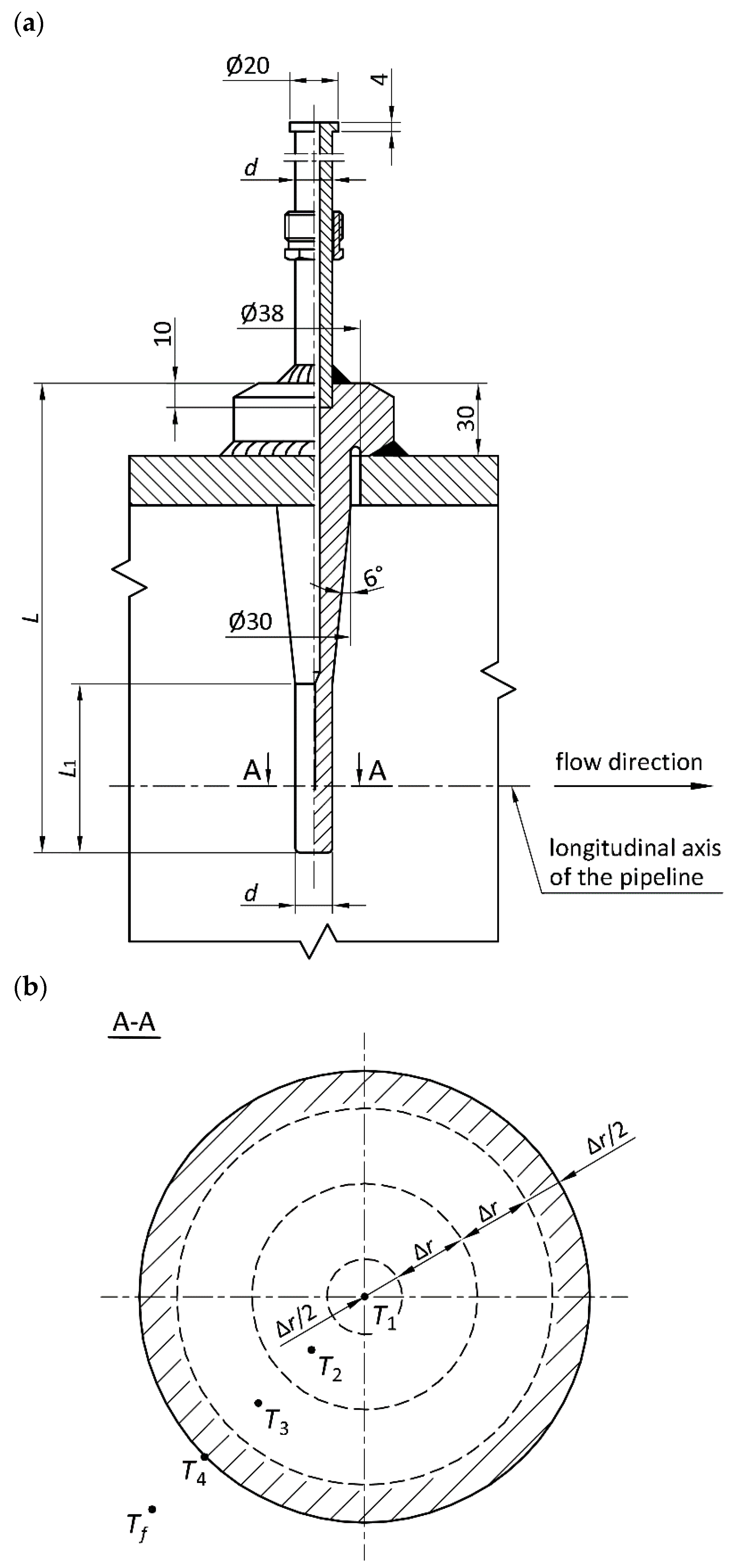
A new fast-response thermometer was designed without the disadvantages of the conventional thermometer described above. The massive housing of the thermometer was replaced by a cylinder with a small hole in its axis. In this hole, a thermocouple of the same diameter is placed (Figure 1a), which eliminates the thermal resistance of the air gap. The hole in the cylinder is not drilled to the outlet so that the thermometer is leakproof. The thermocouple junction is located 27.5 mm from the end of the cylinder.

The new-design thermometer was modelled as a full cylinder with an axis temperature known from measurements (Figure 1). With a lack of massive housing and air gap as well as the ceramic insulating beads, the thermometer has excellent dynamic properties.

2. Inverse Method to Obtain the Accurate Transient Temperature of the Fluid

The inverse space marching method was used to determine the temperature distribution in the solid cylinder and the temperature of the fluid. The equation of the transient heat conduction in a cylindrical wall is expressed by:

$$c\left(T\right)\rho \left(T\right)\frac{\partial T}{\partial t}=\frac{1}{r}\frac{\partial }{\partial r}\left[k\left(T\right)r\frac{\partial T}{\partial r}\right],\hspace{1em}0\le r\le r_{out}$$

(1)

where c is specific heat (J/(kg·K)), ρ is density (kg/m³), T is temperature (K), t is time (s), r is radius (m), k is thermal conductivity (W/(m·K)) and r_out is radius of the outer surface (m).

From the measured temperature T₁(t) at the axis of the cylinder r = 0:

$$T\left(r=0\right)=T_1(t)$$

(2)

The transient temperature distribution inside the cylinder wall including the outer surface will be determined.

Since the problem is axisymmetric, the heat flux in the axis of the cylinder is equal to zero, i.e.,

$${\frac{\partial T}{\partial r}|}_{r=0}=0$$

(3)

The unknown temperature of the fluid T_f (t) occurs in the convective boundary condition on the external surface of the thermometer casing:

$$k(T){\frac{\partial T}{\partial r}|}_{r=r_{out}}=h\left(t\right)\left(T_f-{T|}_{r=r_{out}}\right)$$

(4)

where h is heat transfer coefficient at the thermometer surface (W/(m²K)).

The value of the heat transfer coefficient at a given time h(t) depends on temporary changes in the mass flow or pressure of the fluid. The heat transfer coefficient h on the surface of the thermometer casing was calculated with the formula proposed by Churchill [18] for a single cylinder transversely flowing through the liquid.

The boundary condition (4) does not take into account the radiation between the thermometer and the surrounding surfaces. Radiation can have a significant effect on the results of measurements, for gaseous flow when the thermometer temperature is higher than the temperature of the surrounding surfaces. In this case, the boundary condition must take into account the heat transfer by radiation between the thermometer and the wall of the pipeline or between the thermometer and the anti-radiation shield wall, which allows the radiation heat transfer to be reduced.

The inverse heat conduction problem (1)–(3) will be solved by using the finite volume method (FVM) [19]:

$$\Delta V_{i}c\left(T_i\right)\rho \left(T_i\right)\frac{\mathrm{d}{T}_i}{\mathrm{d}t}={\displaystyle \sum _{j=1}^{n_c}{\dot{Q}}_{i,j}+\Delta V{\dot{q}}_v\left(T_i\right)}$$

(5)

where ΔV_i is volume of single cell (control volume) with the node under consideration (m³), T_i is temperature at the ith node (°C), n_c is number of cells adjacent to a cell i (−), ${\dot{Q}}_{i,j}$ is heat flow rate from neighboring node j to the node i (W), ΔV is volume of single cell (control volume) (m³) and ${\dot{q}}_v$ is energy generation rate per unit volume (uniform within the body) (W/m³).

The casing of the thermometer has been modeled as a solid cylinder. The computational domain is divided into four control volumes (Figure 1b). For all nodes, located at the centers of the control volumes, the energy balance equations were written.

The surface temperature T₄ was determined in sequence. Time changes of temperature in time at point 1 T₁(t) were measured, so the temperature at node 2 was determined from the equation of the energy balance at node 1:

$$T_2=T_1+\frac{1}{2}\frac{{\left(\Delta r\right)}^2}{k\left(T_1\right)+k\left(T_2\right)}c\left(T_1\right)\rho \left(T_1\right)\frac{\mathrm{d}{T}_1}{\mathrm{d}t}$$

(6)

By calculating the time derivative dT₁/dt and using Equation (6), the temperature at node 2 was obtained at first.

Next, the temperature at node 3 was determined using the energy balance equation at node 2. After calculating the derivative dT₂/dt, the temperature in node 3 was calculated from the following equation:

$$T_3=T_2-\frac{1}{3}\frac{k\left(T_1\right)+k\left(T_2\right)}{k\left(T_3\right)+k\left(T_2\right)}\left(T_1-T_2\right)+\frac{4}{3}{\left(\Delta r\right)}^2\frac{c\left(T_2\right)\rho \left(T_2\right)}{k\left(T_3\right)+k\left(T_2\right)}\frac{\mathrm{d}{T}_2}{\mathrm{d}t}$$

(7)

Finally, the temperature at node 4 could be calculated using the heat balance equation and the time derivative dT₃/dt for node 3:

$$T_4=T_3-\frac{3}{5}\frac{k\left(T_2\right)+k\left(T_3\right)}{k\left(T_4\right)+k\left(T_3\right)}\left(T_2-T_3\right)+\frac{8}{5}{\left(\Delta r\right)}^2\frac{c\left(T_3\right)\rho \left(T_3\right)}{k\left(T_4\right)+k\left(T_3\right)}\frac{\mathrm{d}{T}_3}{\mathrm{d}t}$$

(8)

where the symbol Δr = r_out/3 denotes the spatial step in the r direction in m.

The energy balance equation for node 4 is as follows:

$$\pi \left[r_{out}^2-{\left(r_{out}-\frac{\Delta r}{2}\right)}^2\right]c\left(T_4\right)\rho \left(T_4\right)\frac{\mathrm{d}{T}_4}{\mathrm{d}t}=2\pi \left(r_{out}-\frac{\Delta r}{2}\right)\frac{k\left(T_3\right)+k\left(T_4\right)}{2}\frac{T_3-T_4}{\Delta r}+2\pi r_{out}h\left(T_f-T_4\right)$$

(9)

After the calculation of temperatures T₂, T₃, and T₄, the fluid temperature T_f (t) was calculated using Equation (10):

$$T_f=T_4-\frac{5}{12}\frac{k\left(T_3\right)+k\left(T_4\right)}{h\Delta r}\left(T_3-T_4\right)+\frac{11}{24}\Delta r\frac{c\left(T_4\right)\rho \left(T_4\right)}{h}\frac{\mathrm{d}{T}_4}{\mathrm{d}t}$$

(10)

The thermal conductivity values k(T_i) for nodes temperatures T_i (where i = 2, 3, 4) in the Equations (6)–(10) are not known. The calculation of the nodal temperature requires several iteration steps. It can be assumed that the initial value of the thermal conductivity in the first iteration is:

$$k\left(T_i^{(0)}\right)=k\left(T_{i-1}\right)$$

(11)

Iterative calculations continued until the following condition was met:

$$\left|T_i^{\left(n+1\right)}-T_i^{\left(n\right)}\right|\le \epsilon ,\hspace{1em}i=2, 3, 4$$

(12)

for a suitably low tolerance value ε or to reach the set number of iterations.

A characteristic feature of the IHCP method is that, unlike direct methods, increasing the number of control volumes does not increase the accuracy of the method [20]. In an analytical-numerical solution of the inverse heat conduction problem, the order of the highest time derivative of the measured temperature is equal to the number of finite volumes into which the domain under study is divided. If a third order polynomial is used to approximate temporary temperature changes, then the number of control volumes must not be greater than the approximation polynomial order, i.e., in this case greater than three. Unlike other methods, the IHCP method does not require knowledge of the initial temperature distribution in a solid cylinder.

3. Computational Validation of the Inverse Method

The method presented in the article has been used to determine the transient fluid temperature changes. First, data was generated by solving a direct heat conduction problem in the cylinder. A case of a linear and stepwise fluid temperature rise was examined. The Duhamel integral was used to simplify the determination of transient temperature distribution when the fluid temperature increases with a constant rate. The case of a stepwise increase in temperature was solved using an analytical method [19].

In the first case, it was assumed that the fluid temperature changes from 0 to 170 °C with a constant rate of temperature change v_T = 0.33333 K/s. In the second case, the fluid temperature jump from the initial value 20 °C to the temperature of 100 °C was assumed. The following thermal properties are assumed for the thermometer made of austenitic steel 1.4541: k = 18 W/(m K), c = 500 J/(kg K), ρ = 7.9 × 10³ kg/m³. The outer diameter of the thermometer is 7 mm. The heat transfer coefficient is equal to h = 2000 W/(m² K) at the outer surface.

Temperature distribution T₁(t) determined by direct methods was the input data for inverse analysis. The value of the time step was obtained from the following condition [19]:

$$\Delta t\ge 0.05 r_{out}^2/\alpha$$

(13)

where: α stands for the thermal diffusivity: α = k/(c·ρ).

In the calculation, a time step of 0.2 s was assumed.

In Figure 2 and Figure 3, the transient temperature variations obtained by direct methods were compared with the solution obtained using the presented inverse solution.

The results of the calculations, depicted in Figure 2 and Figure 3, show a very good coincidence between the temperature changes over time, determined using the inverse method and the results of direct calculations.

4. Experimental Verification of a New Measuring Technique

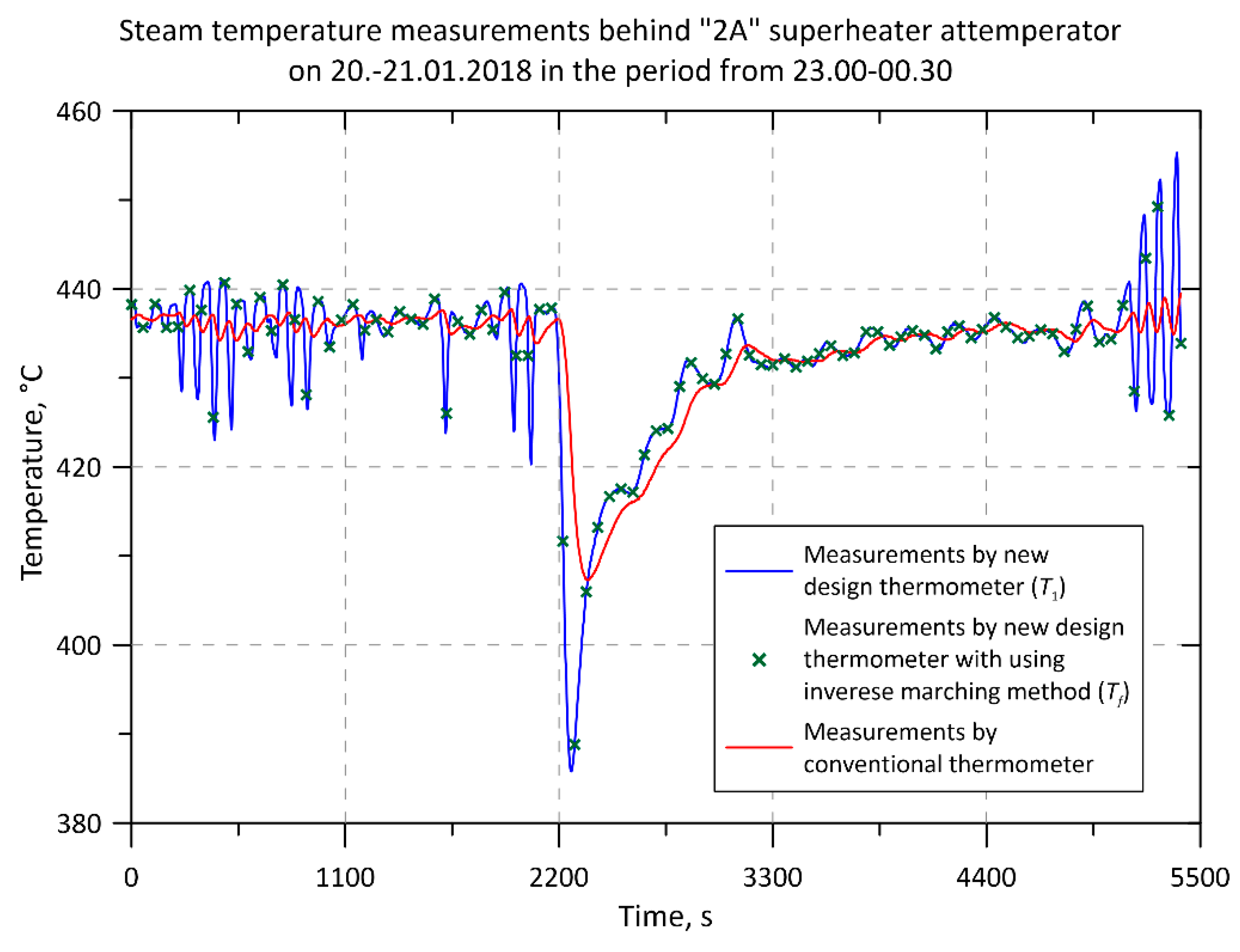
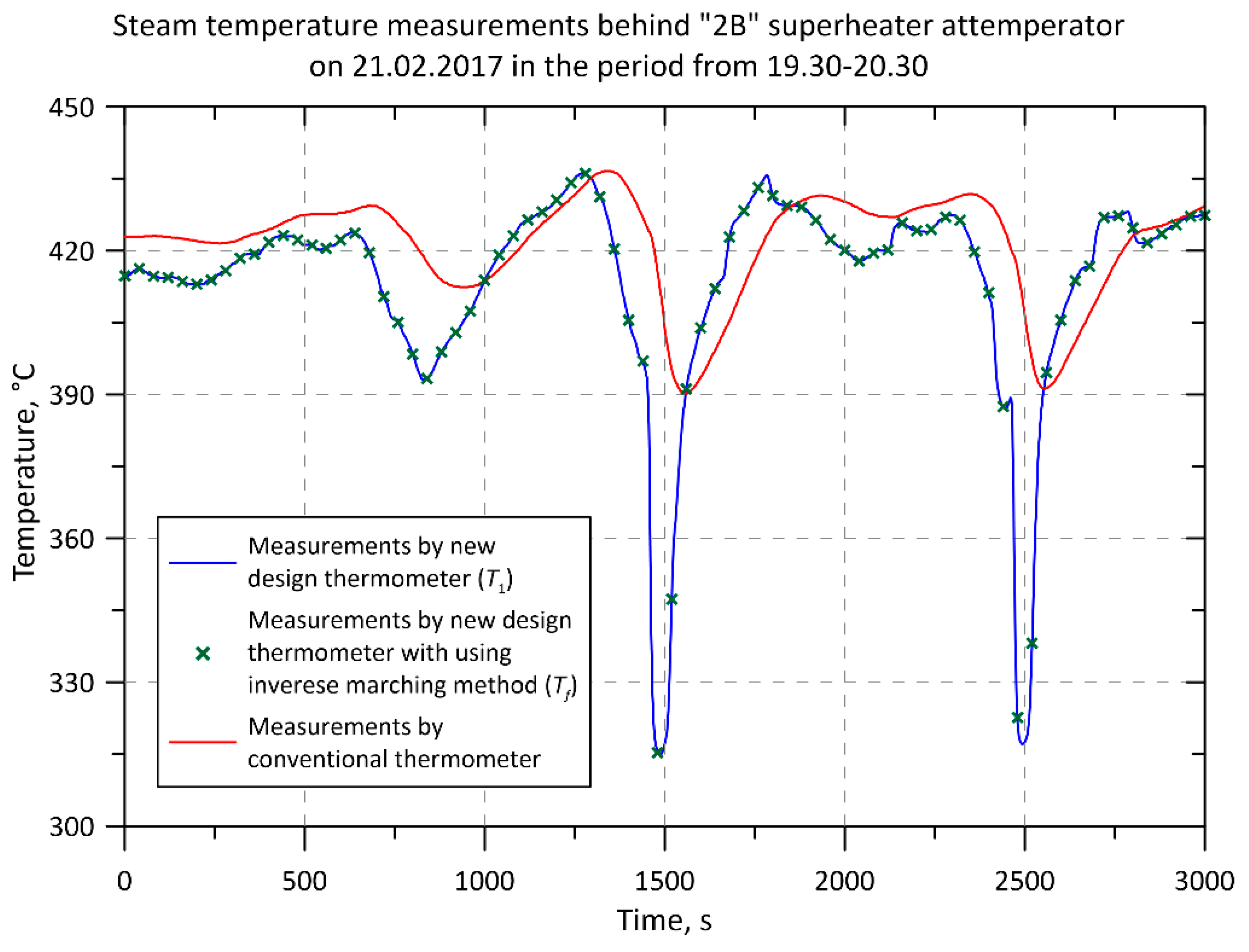
This section presents the experimental results of transient steam temperature measurements carried out with a thermometer of new construction at the Power Plant CEZ Skawina SA. The tests were carried out on the OP-210M boilers with numbers K11 and K8. These are steam boilers fired with hard coal with output of 210 × 10³ kg/h. The thermometers are installed on the outlet header, behind the second attemperators on the A and B side of the boiler. The Figure 4, Figure 5, Figure 6, Figure 7, Figure 8, Figure 9, Figure 10 and Figure 11 show the results of a comparison of time changes registered by the thermometers of the new design with the responses of conventional thermometers installed in the pipelines on the A and B side of the boiler. The curves shown in the Figure 4, Figure 5, Figure 6, Figure 7, Figure 8, Figure 9 and Figure 11 include the moment of water injection on the steam regulators. 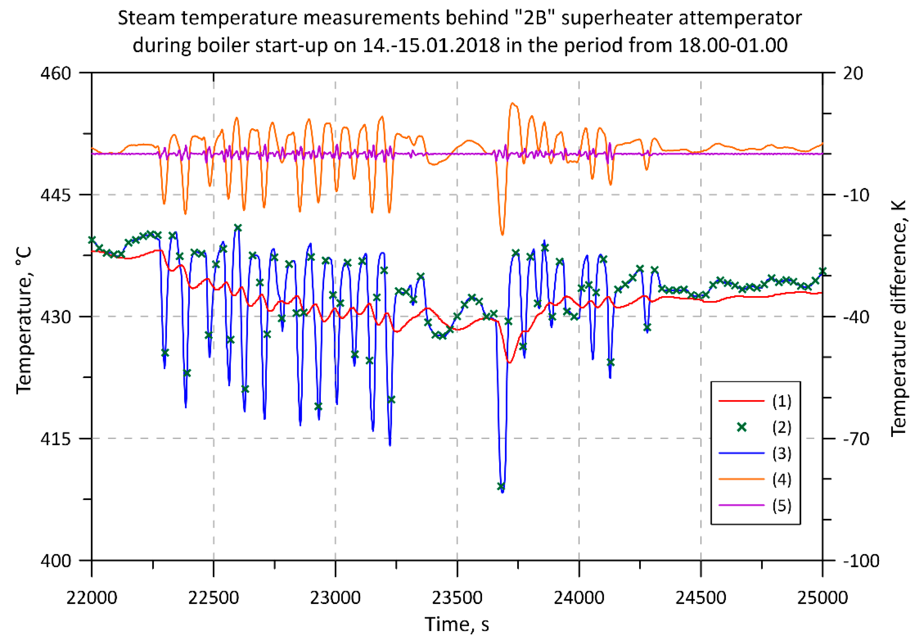Figure 10 shows changes in steam temperature during start-up.

The heat transfer coefficient on the external surface of the new design thermometer necessary to determine the steam temperature using the inverse method was determined using the correlation of Churchill and Bernstein [18]. Depending on the Reynolds number Re and for Re·Pr > 0.2, the correlations have the following form:

– Re > 400,000

$$\mathrm{Nu}=0.3+\frac{0.62{\mathrm{Re}}_{}^{1/2}{\mathrm{Pr}}^{1/3}}{{\left[1+{\left(0.4/\mathrm{Pr}\right)}^{2/3}\right]}^{1/4}}{\left[1+{\left(\frac{\mathrm{Re}}{282000}\right)}^{5/8}\right]}^{4/5}$$

(14)

– 10,000 < Re < 400,000

$$\mathrm{Nu}=0.3+\frac{0.62{\mathrm{Re}}_{}^{1/2}{\mathrm{Pr}}^{1/3}}{{\left[1+{\left(0.4/\mathrm{Pr}\right)}^{2/3}\right]}^{1/4}}\left[1+{\left(\frac{\mathrm{Re}}{282000}\right)}^{1/2}\right]$$

(15)

– Re < 10,000

$$\mathrm{Nu}=0.3+\frac{0.62{\mathrm{Re}}_{}^{1/2}{\mathrm{Pr}}^{1/3}}{{\left[1+{\left(0.4/\mathrm{Pr}\right)}^{2/3}\right]}^{1/4}}$$

(16)

where the symbol Nu denotes the Nusselt number, and Re and Pr are the Reynolds and Prandtl number, respectively.

The values of the heat transfer coefficient changed significantly during the boiler operation. For the measurements shown in Figure 4, Figure 5, Figure 6, Figure 7, Figure 8, Figure 9, Figure 10 and Figure 11, during continuous boiler operation, the heat transfer coefficient was equal to about 3000 W/(m²K), while during the injection of water into the steam stream increased up to about 6300 W/(m²K). At high velocity fluid flow, the heat transfer coefficient is also high, resulting in a small temperature difference between the outer surface of the thermometer and the fluid temperature. Even imprecise determination of the heat transfer coefficient does not result in large errors in measuring the temperature of the fluid.

The descriptions in the legends in Figure 4, Figure 5, Figure 6, Figure 7, Figure 8, Figure 9 and Figure 10 are as follows. “Measurements by new design thermometer (T₁)” and “Measurements by conventional thermometer” denote temperatures measured by new and conventional thermometers, i.e., temperatures indicated by temperature sensors (thermocouples) located inside these thermometers. The description: “Measurements by new design thermometer with using the inverse marching method (T_f)” means the steam temperature that was determined using an inverse solution based on the readings of the thermocouple in the axis of the new thermometer.

The analysis of measurement results (Figure 4, Figure 5, Figure 6, Figure 7, Figure 8, Figure 9, Figure 10 and Figure 11) of the transient steam temperature shows that the thermometer of the new construction has a much smaller dynamic error than the conventional thermometer. The biggest differences in thermometer indications can be observed during water injection on the temperature regulator (Figure 4, Figure 5, Figure 6, Figure 7, Figure 8, Figure 9 and Figure 11). The biggest difference in indications between the thermometer of the new and old construction is over 39 K (Figure 4) and 97 K and 93 K (Figure 7). Figure 4 and Figure 7 show the temperature indicated by the thermocouple located in the axis of the new thermometer (solid blue line) and the temperature of steam determined from the solution of the inverse problem (green crosses). Differences between these temperatures are small due to the high values of the heat transfer coefficient on the outer surface of the thermometer. The difference between the temperature of the steam determined from the inverse solution and the temperature of the thermocouple in the new thermometer is shown in Figure 6 and Figure 9. It can be seen that the value of this difference was in the range of −8 K to about 7 K (Figure 9), and in the case of the results shown in Figure 6 even smaller and ranged from about −1.5 K to 2 K. The larger differences between the temperature measured with the new thermometer and the temperature obtained using the inverse method shown in Figure 9 are caused by a bigger (in this case about 75 K) and a more rapid drop in the temperature of superheated steam. The new thermometer has thermal inertia, although small. Using the inverse method allows the temperature indicated by the thermocouple placed in the axis of the new thermometer to be corrected.

During boiler start-up, when the temperature of steam rises (Figure 10), the thermometer of the new design reacts more quickly to the increase in the temperature of the medium and shows higher temperature values. The situation is similar when the boiler is shut down. The new design reacts more quickly to a decrease in steam temperature showing lower values than the conventional design. Differences in indications of both thermometers during start-up and shutdown, due to the nature of temperature changes, are smaller than during water injection but are still very large.

In the analyzed cases, the steam temperature determined from the solution of the inverse problems differs little from the center temperature of the cylinder (Figure 4, Figure 5, Figure 6, Figure 7, Figure 8, Figure 9 and Figure 11). This is due to the small diameter of the cylinder (2r_out = 15 mm) inside which the thermocouple is placed and the high thermal conductivity of the thermometer material of about 35 W/(mK). The main reason for the small difference between the steam temperature and the center of the cylindrical part of the thermometer is, however, the high heat transfer coefficient on the outer surface of the thermometer. The high value of the heat transfer coefficient results, in turn, from the high steam velocity.

Despite the small differences between the temperature indicated by the new thermometer and the calculated temperature, it is recommended to use the inverse method during measurements. As the tests presented in [21] show, the thermal resistance on the external surface of the thermometer can be significant at lower fluid velocities. This may cause the temperature indicated by the thermometer to deviate from the actual temperature. Application of the inverse method allows to increase the accuracy of measurement of transient fluid temperature.

Figure 11 illustrates changes in steam temperature caused by incorrect operation of the proportional-integral-derivative (PID) controller used to maintain a constant temperature behind the second stage of the steam superheater in the K8 boiler.

PID controller settings such as coefficients for the proportional, integral, and derivative terms are set for clean, ash-free superheater tubes. Initially, the operation of the PID regulator is stable, but as the superheater gets fouled with ash, the operation of the regulator becomes unstable (Figure 11). The conventional thermometer is not able to detect abnormal operation of the regulator due to its very high inertia. The new thermometer shows the actual superheated steam temperature changes that cause cyclic thermal stress in the steam cooler chamber. It is necessary to remove the ash from the external surfaces of the superheater tubes to restore proper operation of the PID controller or to select new settings of the PID controller so that it will operate stably. As a result of the faulty operation of the PID controller, steam temperature fluctuations are significant. The lifetime of elements of a superheater operating in such conditions will be lower.

5. Strength Analysis

As shown in the previous chapters, the indications of the thermometer of the new design differ significantly from those of the conventional thermometer. The most significant differences are during sudden fluid temperature changes. In this chapter, the influence of the thermometer readings on the results of stress field calculations in a pressure element was analyzed. A coupled transient thermal-strength analysis was carried out for the outlet header of the boiler K11 on which the thermometer of the new construction has been installed. The outer radius of the header is 0.1365 m, and the wall thickness is 0.02 m. In the wall of the header, there is an opening with a radius of 0.0285 m. The header is made of boiler steel with a grade 13HMF (DIN symbol: 14MoV63). Figure 12 and Figure 13 show changes of the thermophysical properties as a function of temperature which were used in the calculations.

Thermal analysis was carried out for time changes in steam temperature according to the indications of the conventional and the new construction thermometer, as shown in Figure 14. For the temperature time changes the heat transfer coefficient on the inner surface of the header was calculated respectively for the indications of the new design and standard thermometers (Figure 14). Figure 15 shows changes in the steam pressure and mass flow rate.

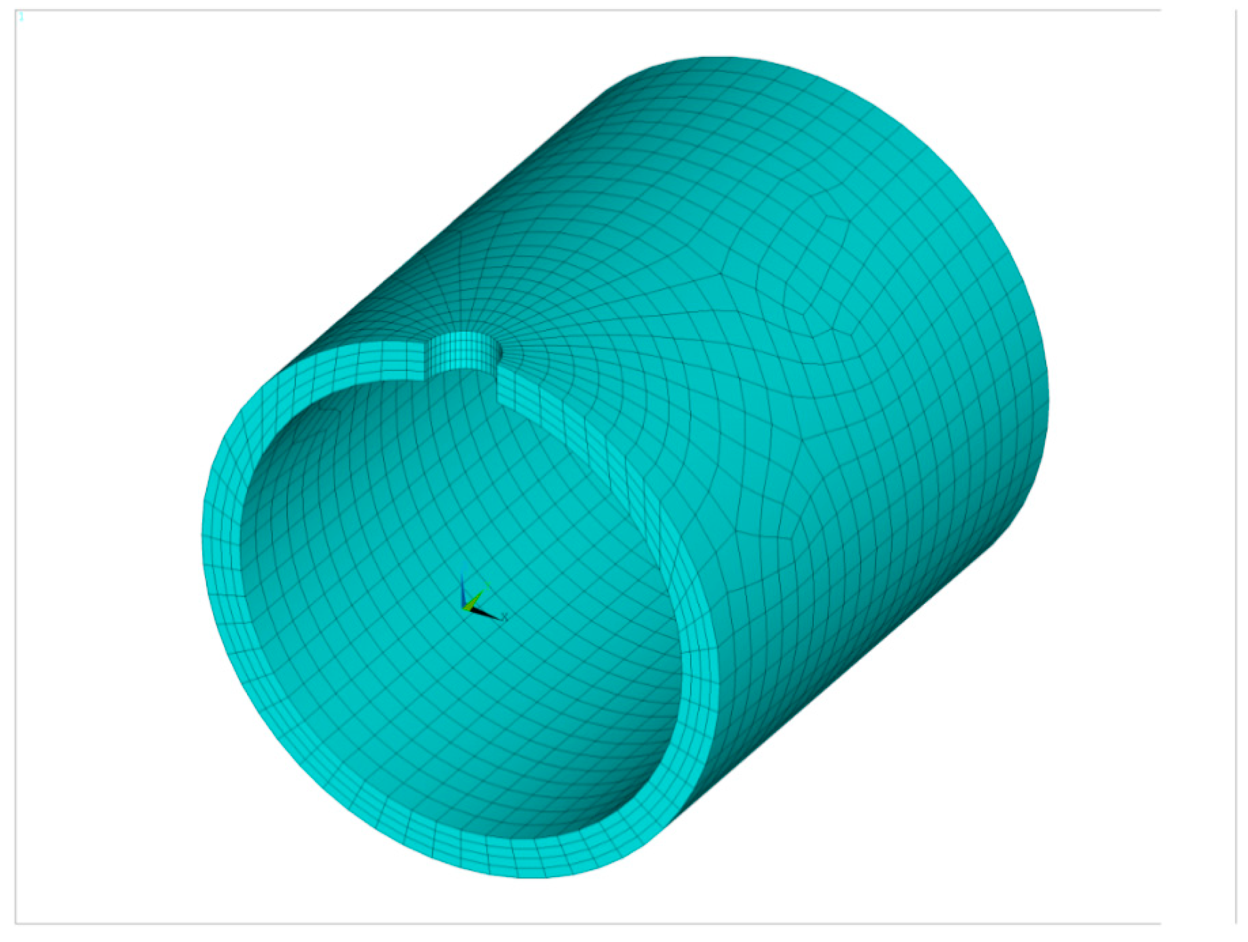
The analyses of temperature and stress fields were carried out using the FEM Ansys 19.1 package [22]. A sequential analysis was carried out, the first stage of which is the solution of the heat transfer issue. The temperature determined was then used in the strength analysis. Figure 16 shows a finite element mesh that was used in calculations.

The maximum difference in the thermometers indication was equal to 96.9 K (Figure 14) after water injection. The analysis of the results depicted in Figure 14 shows significant differences between the heat transfer coefficients calculated using the indications of the new and the conventional thermometer. For 688 s (Figure 14), the value of the heat transfer coefficient was 1385 W/(m²K) when the fluid temperature indicated by the conventional thermometer was used. This value is three times lower than the value of the coefficient equal to 4160 W/(m²K), which was calculated using indications of the thermometer of the new design.

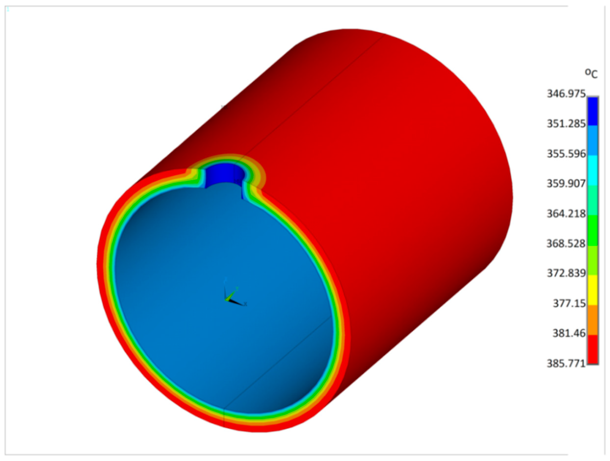
Figure 17 shows the temperature field after 688 s. Significant cooling of the header wall during water injection can be observed due to the relatively small wall thickness and the high value of heat transfer coefficient. The steady temperature of the header before water injection was about 414 °C.

Figure 18 illustrates the von Misses stress field for the same moment in time. The stress value reaches its highest value for a time of 688 s. The highest stress value occurs for a time of 740 s for the calculation according to the indications of a standard thermometer.

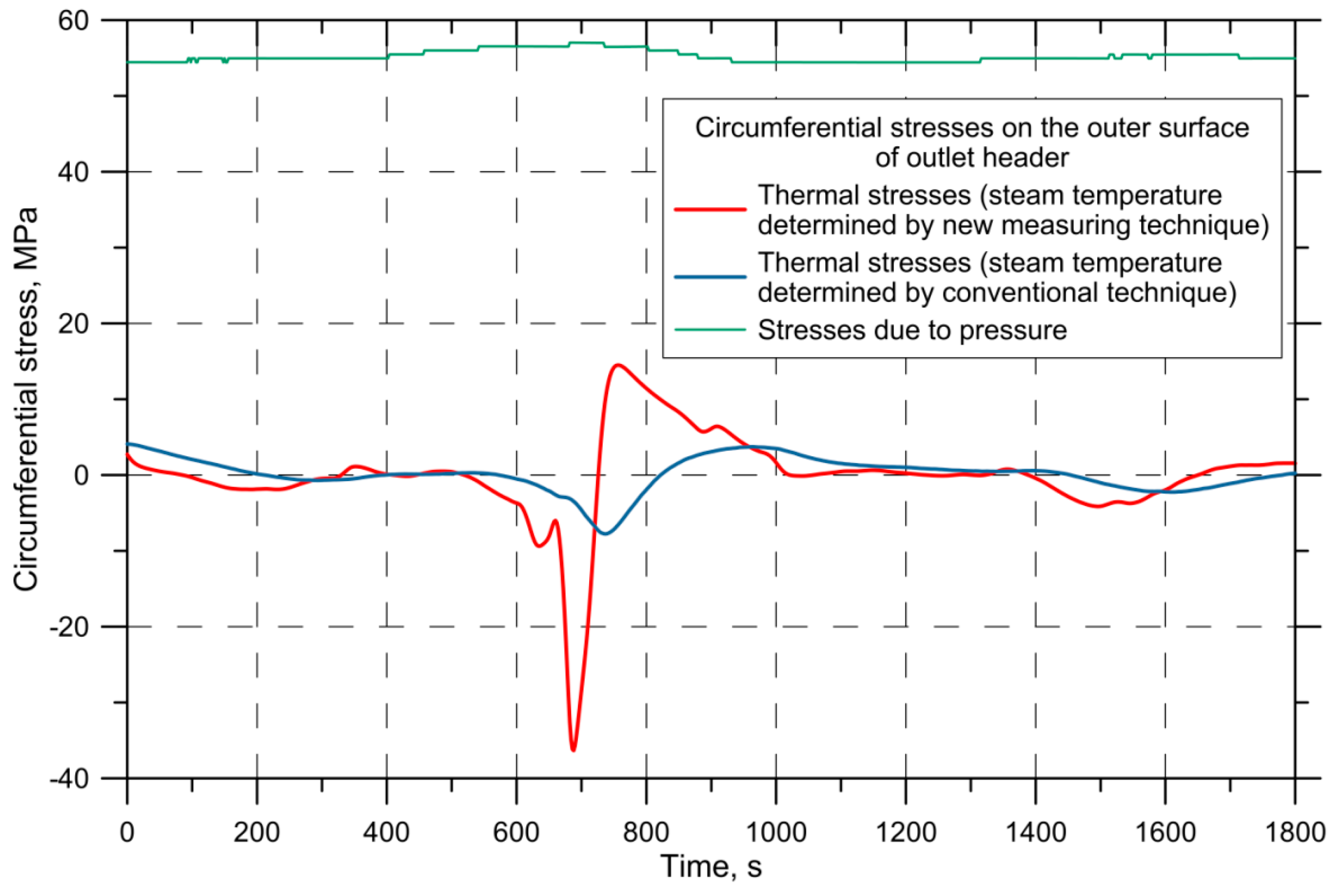
Practice shows that damage to pressure elements are most often radial cracks around the hole starting from the inner surface. Thermal stresses are caused by uneven temperature distribution in axial, radial and circumferential directions. Circumferential stresses on the opening edges are particularly dangerous. They can exceed the permissible stresses during temperature peaks and cause plastic deformation of the edges of the holes. This results in fatigue or creep damage. Figure 19 and Figure 20 show time variations in circumferential stresses on the inner and outer surface of the header in the cylindrical part, at a significant distance from the hole.

The maximum value of the circumferential thermal stresses is according to the new measuring technique four times greater than the maximum circumferential stress caused by temperature changes according to the conventional method. These peaks are also delayed in time, as are the indications of changes in temperature. At the moment of water injection, on the inner surface of the header, the values of circumferential thermal stresses may exceed the values of stresses from pressure. In addition, high differences in the calculated values of circumferential thermal stresses occur at the edge of the hole at the stress concentration point (Figure 21). In this case, the highest circumferential stress is the stress due to pressure, which occurs at the edge of the hole.

6. Conclusions

The measurements of superheated steam temperature changes over time demonstrated excellent dynamic properties of the thermometer of the new construction. The difference in the readings of the conventional thermometer in relation to the indications of the proposed thermometer achieved 100 K. This difference was reached immediately after water injection into the steam stream. In case of sudden changes in steam temperature, the classic thermometers used by boilers manufacturers are not able to reproduce the actual changes in the fluid temperature, and the dynamic temperature measurement errors are substantial. By selecting the right materials for the thermometer casing and dimensioning, the thermometer of the new design can be adapted to work in a wide range of pressures and temperatures of the fluid.

The paper showed the influence of temperature measurement accuracy on the values of calculated stresses in pressure elements. The new measuring technique, using the thermometer with excellent dynamic parameters, allows measuring transient rapid temperature changes. Such temperature fluctuations lead to stress peaks. The stresses generated in this way, especially circumferential stresses, sum up with circumferential stresses due to pressure and may significantly exceed the permissible stresses. The operating experience shows that circumferential thermal stresses are often 2–3 times higher than circumferential pressure stresses. They cause damage of creep or fatigue type, and most often both types. These are damages related to the way of operation, and accurate temperature measurement allows for precise modelling of strength states inside the pressure element, and in consequence to identify dangerous situations. The application of the new measurement method allows for safer operation of high-temperature pressure installations. The application of the proposed new technique of temperature measurement in superheated steam temperature control systems improves the quality of this regulation significantly.