Impact on Drained Rock Volume (DRV) of Storativity and Enhanced Permeability in Naturally Fractured Reservoirs: Upscaled Field Case from Hydraulic Fracturing Test Site (HFTS), Wolfcamp Formation, Midland Basin, West Texas

Abstract
:1. Introduction
2. Natural Fracture and Hydraulic Fracture Models
2.1. Natural Fracture and Hydraulic Fracture Interaction Mechanisms
- (1)
- Equivalent permeability enhancement: The presence of a natural fracture system open to flow (uncemented) with higher permeability than the matrix, would increase the equivalent permeability of the overall reservoir. This enhanced equivalent permeability will result in a corresponding higher flow rate towards the hydraulically fractured well increasing the well productivity.
- (2)
- Storage effects due to natural fracture enhanced porosity: Natural fracture porosity may differ from the matrix either on initial formation of the fracture or due to later dissolution of precipitated minerals in the fracture space [25]. Due to size dependent sealing patterns, larger natural fractures are believed to have greater porosity [27] and as such, porosity in natural fractures is thought to be underestimated in most models. A greater porosity in the natural fractures than in the matrix may affect the extent of the drained area because porosity is a major control on time of flight for particles traveling along streamlines [28]. If the porous fractures are more fluid-filled than the surrounding matrix, storage effects will affect the well productivity. Uncemented fractures with enhanced porosity will allow for storage of hydrocarbons that, when tapped by the hydraulic fractures, will flow readily towards the well.
- (3)
- Connection of hydraulic fractures to natural fractures: Hydraulic fractures will propagate preferentially along planes of weakness in the reservoir such as those created by natural fracture systems. If a hydraulic fracture reactivates and connects to the natural fracture system, this connection leads to the natural fractures essentially becoming a direct extension of the hydraulic fracture pressure sink. The connection of both fracture systems correspondingly increases the total fracture surface area that is in contact with the reservoir matrix and improves the production rate of such wells.
2.2. Natural Fracture Modeling
2.3. Natural Fracture Porosity and Permeability
3. CAM Solution for Hydraulic Fractures and Natural Fractures
4. Modeling of Natural Fracture Interaction Mechanisms
4.1. Equivalent Permeability Enhancement
4.2. Natural Fracture Storativity Effect
4.3. Natural Fractures as Extension to Hydraulic Fracture Network
5. Results
5.1. Representative Elementary Volume (REV) Models
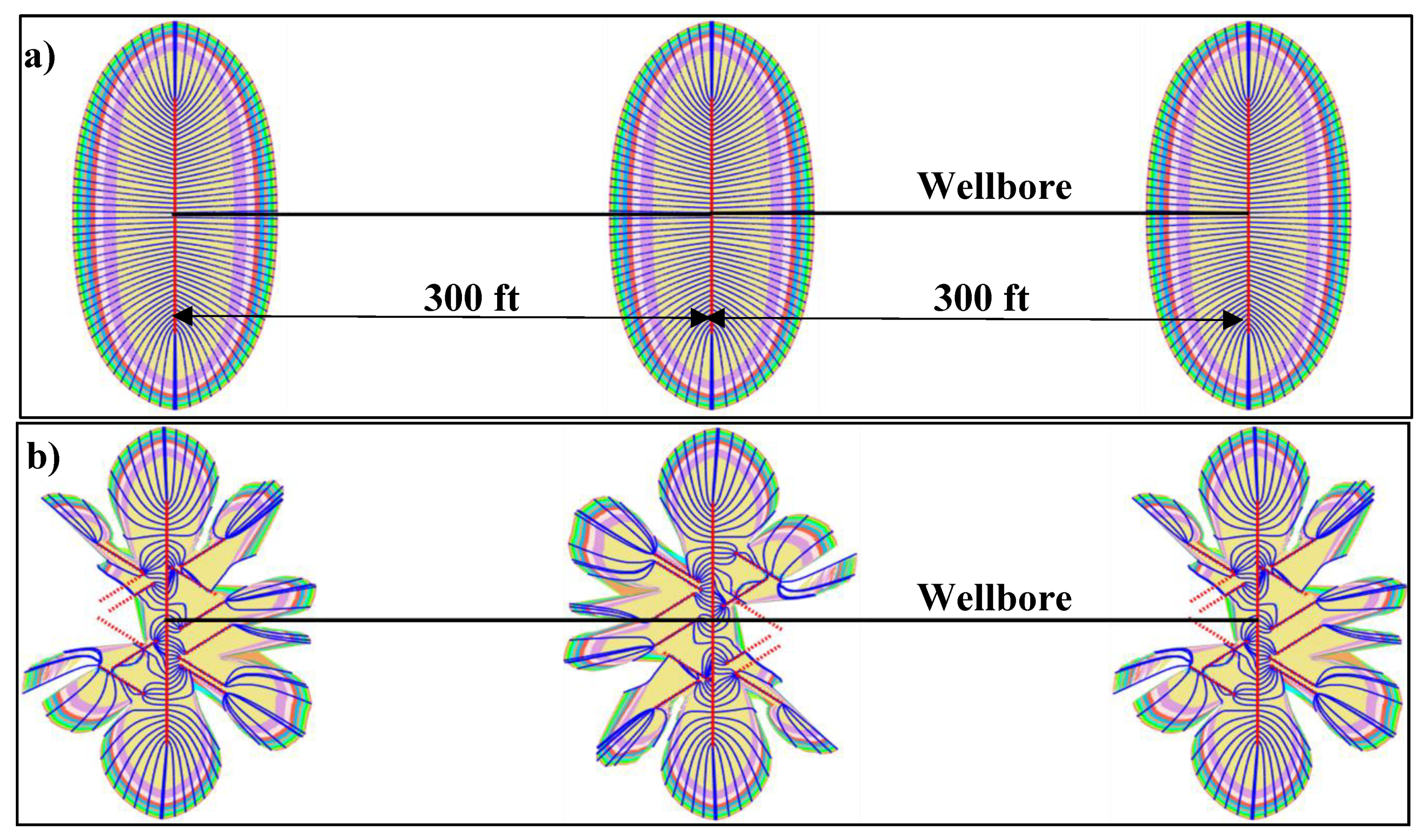
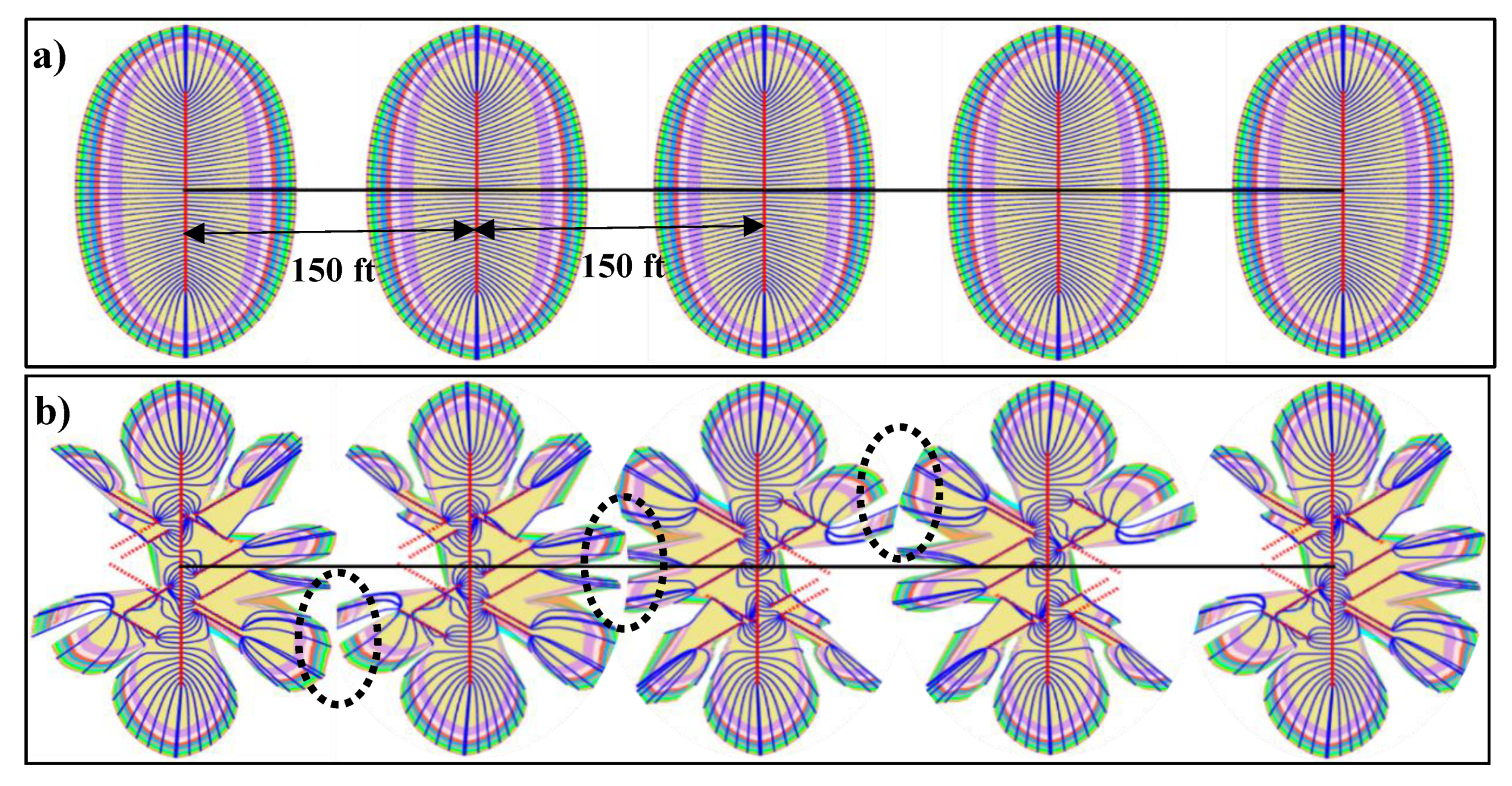
5.2. Synthetic Hydraulic Fracture Models
5.3. Field Models Using Data from the Hydraulic Fracture Test Site (HFTS)
5.4. HFTS Full Well Model and Implications
6. Discussion
6.1. Storativity Impact of Natural Fractures
6.2. Enhanced Permeability vs. Enhanced Storativity
6.3. Model Strengths and Limitations
6.4. Practical Implications
7. Conclusions
- (1)
- Natural fractures can affect reservoir flow through three major mechanisms: (i) by enhancing permeability, (ii) by altering the porosity in the fractures, leading to increased storativity, and (iii) by becoming extensions of the hydraulic fracture network due to reactivation.
- (2)
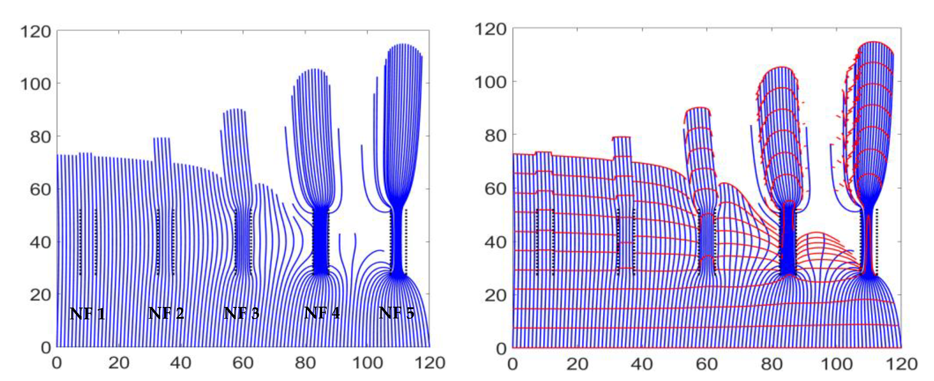
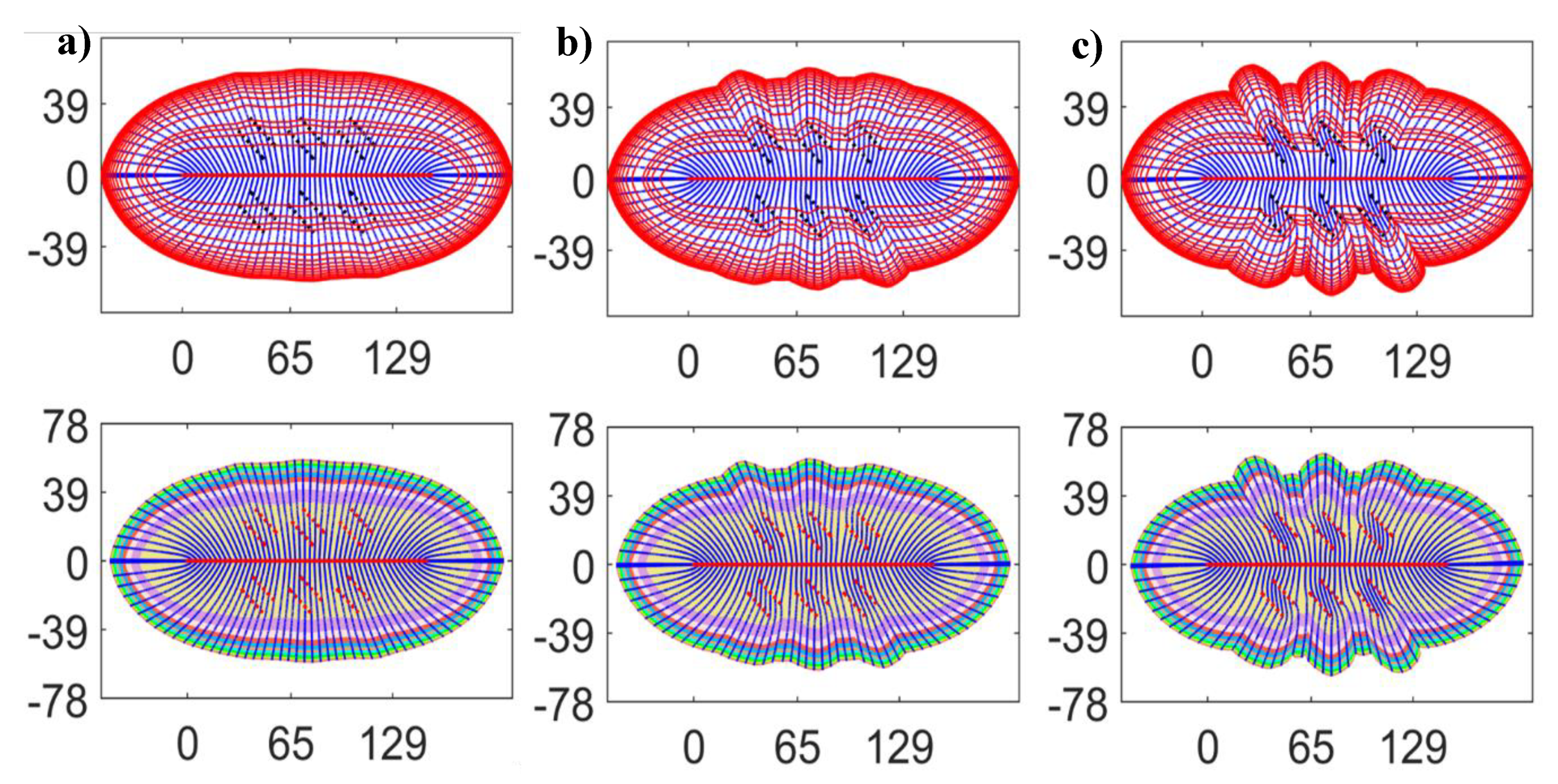
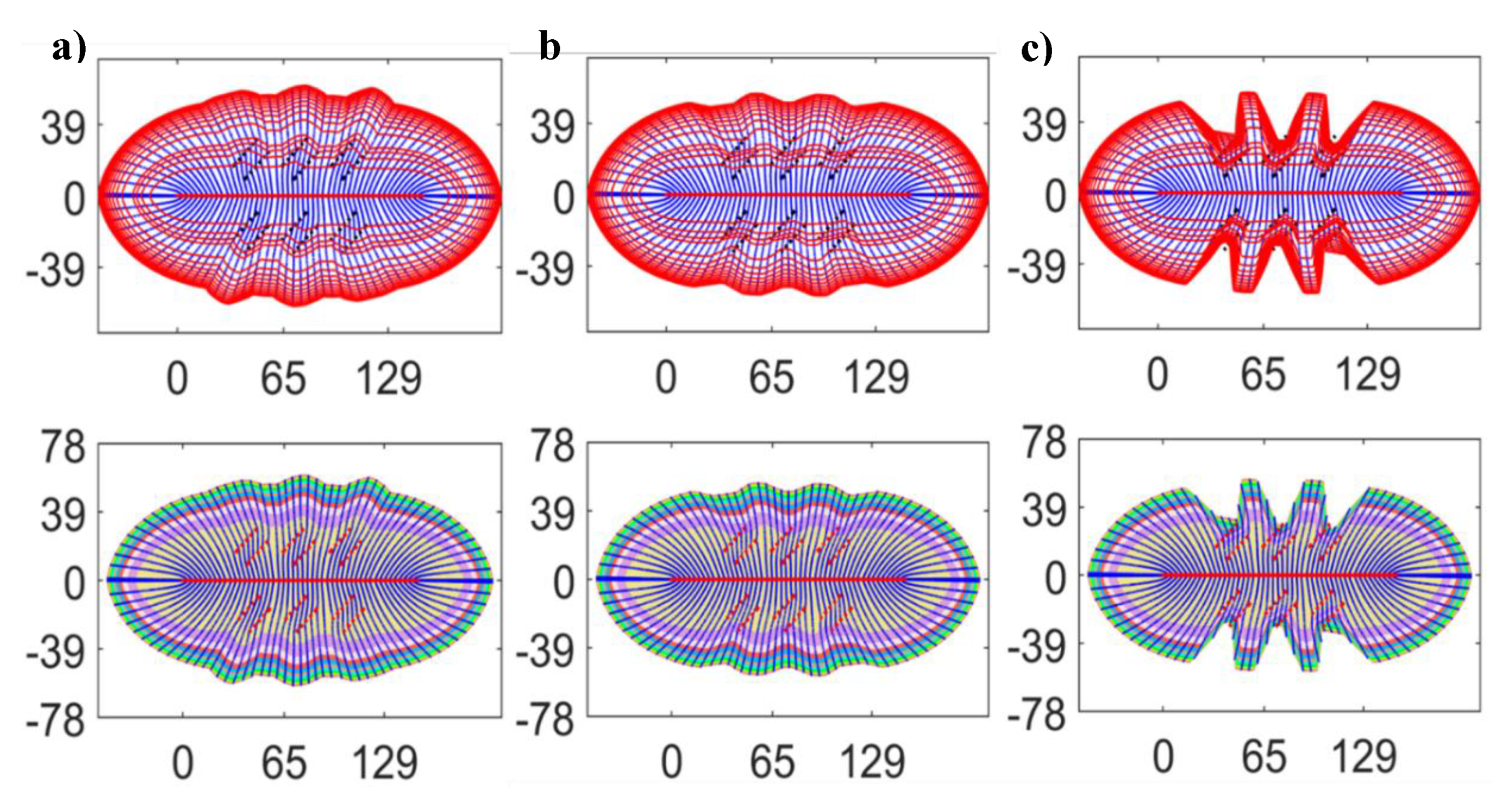
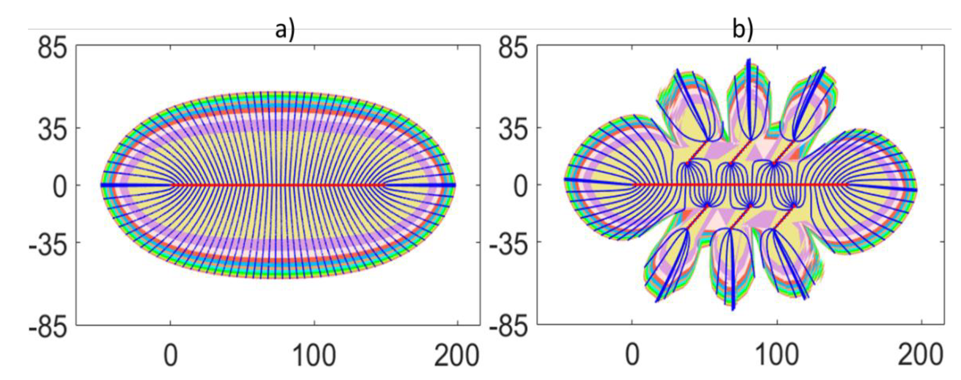
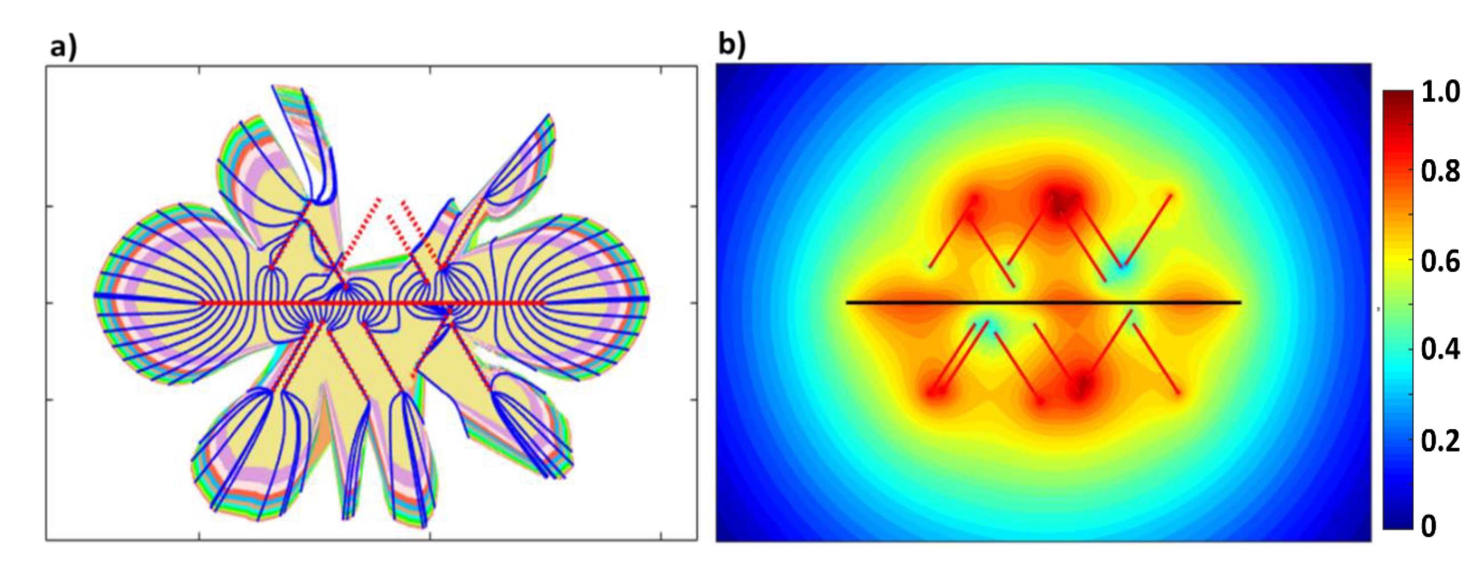
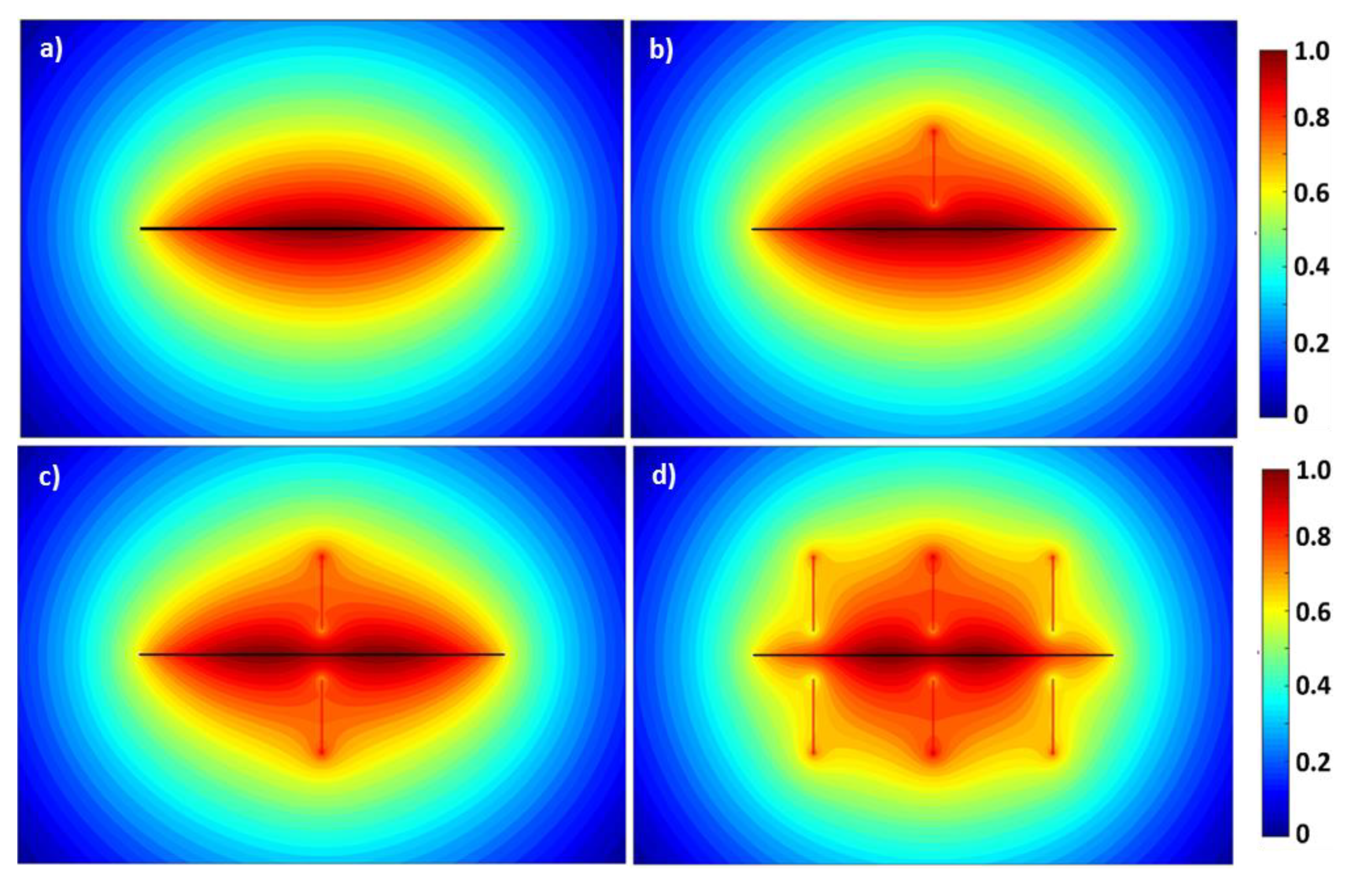
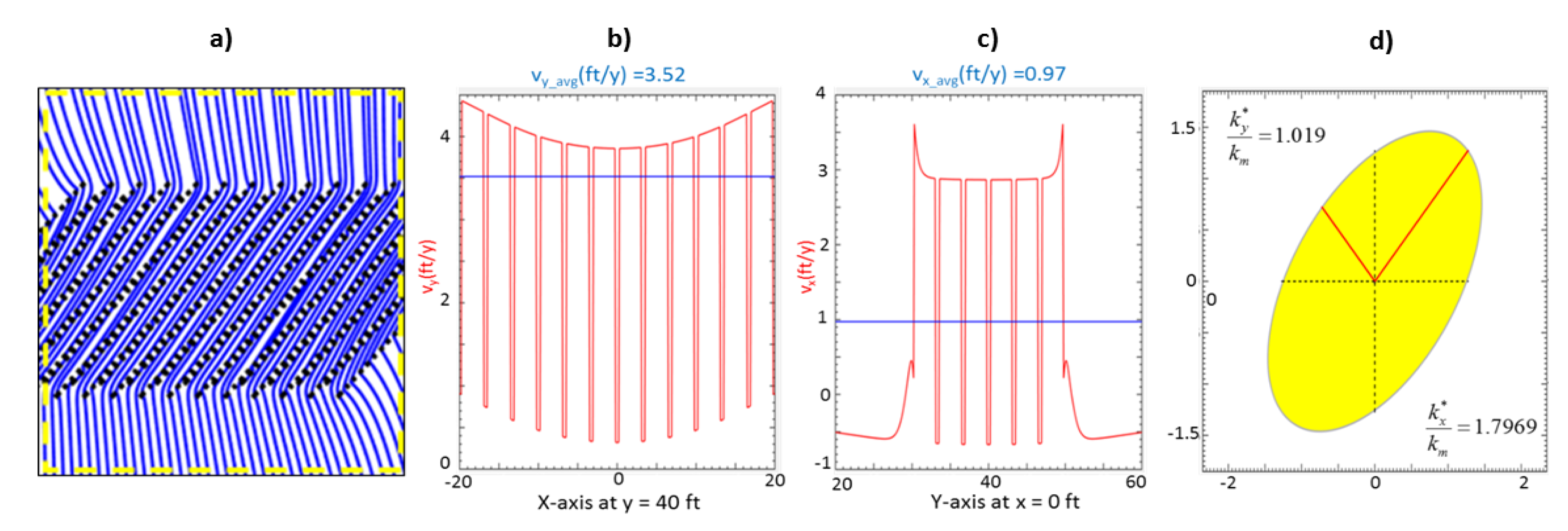
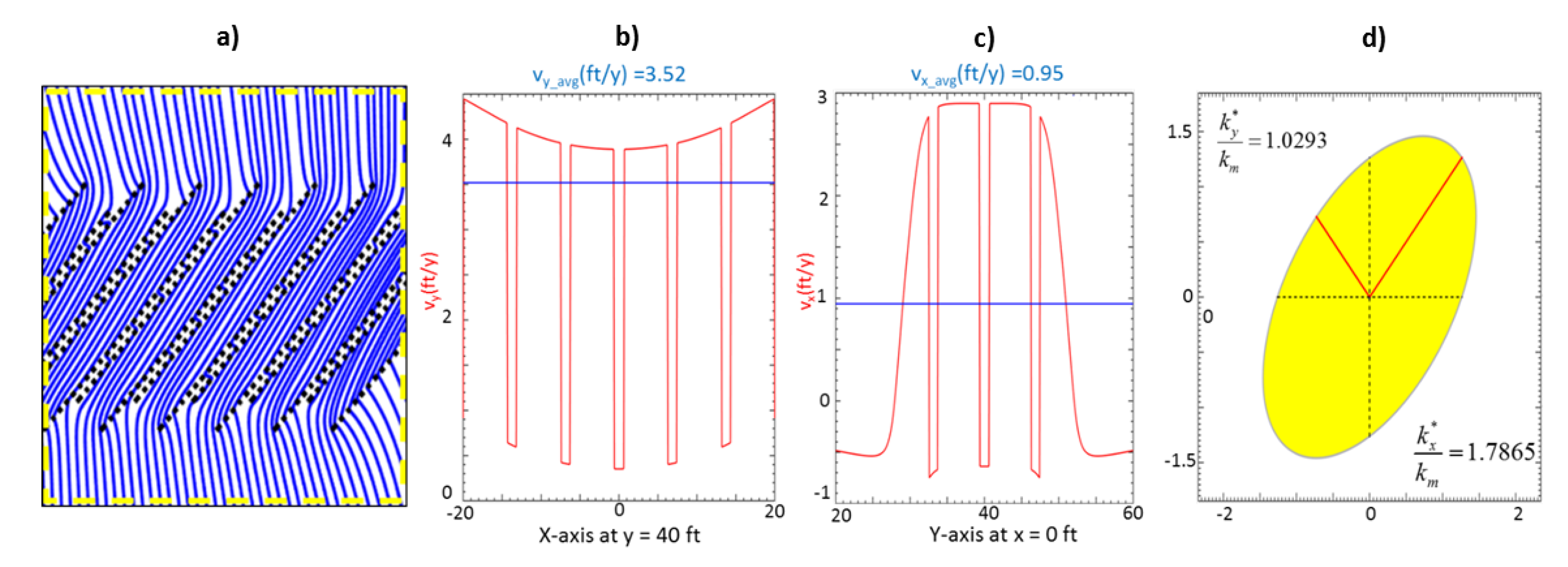
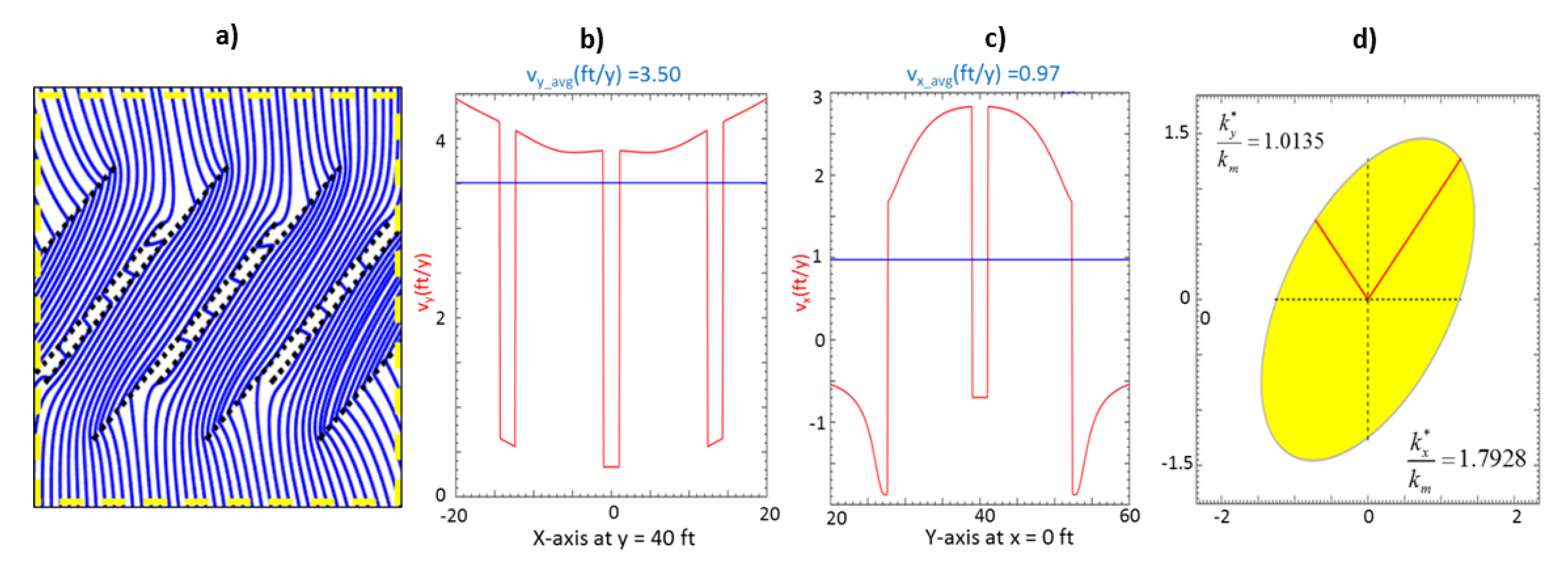
- Enhanced permeability in natural fractures creates high velocity flow zones which preferentially channel fluid flow through them. At high enough permeabilities (or natural fracture strengths as used in our models), this preferential pathway to flow leads to bypassed regions in the matrix blocks between the natural fractures, which are left undrained. These undrained matrix regions can then be targeted by refracturing to improve recovery factors from hydraulically fractured horizontal wells.
- (3)
- Altered porosity or enhanced storativity (due to natural fractures with a higher porosity than the reservoir matrix as investigated in synthetic models) leads to a decrease in the lateral extent of the DRV. The impact of both natural fracture storativity and permeability greatly affect the shape and extent of the DRV around the hydraulic fractures.
- (4)
- The Carman–Kozeny (CK) relation was used to determine the relative impacts of the correlated porosity and permeability in natural fractures on the DRV development. Results based on the CK correlation show that the enhanced flow due to permeability far outweighs any storativity effects (even if natural fractures were to have a higher porosity than the reservoir matrix).
- (5)
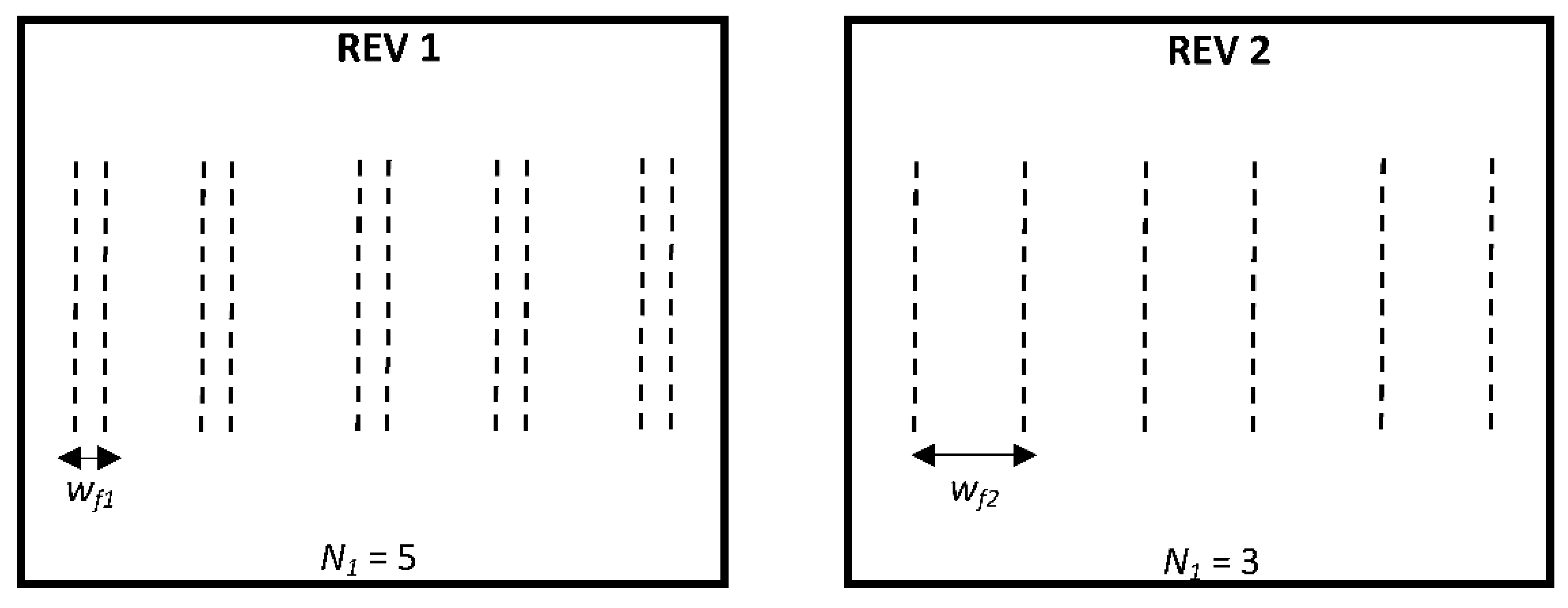
- Use of a hybrid object-based and flow-based method for upscaling allows for the modeling of a high-density natural fracture network. Upscaling is needed to reduce the number of natural fractures modeled while keeping the equivalent permeability the same.
- (6)
- Field data on in-situ natural fracture characteristics such as porosity and permeability is sparse and lacking in the literature. Industry needs to ensure collection of such data for use in reservoir models to accurately determine subsurface flow and drainage volumes.
- (7)
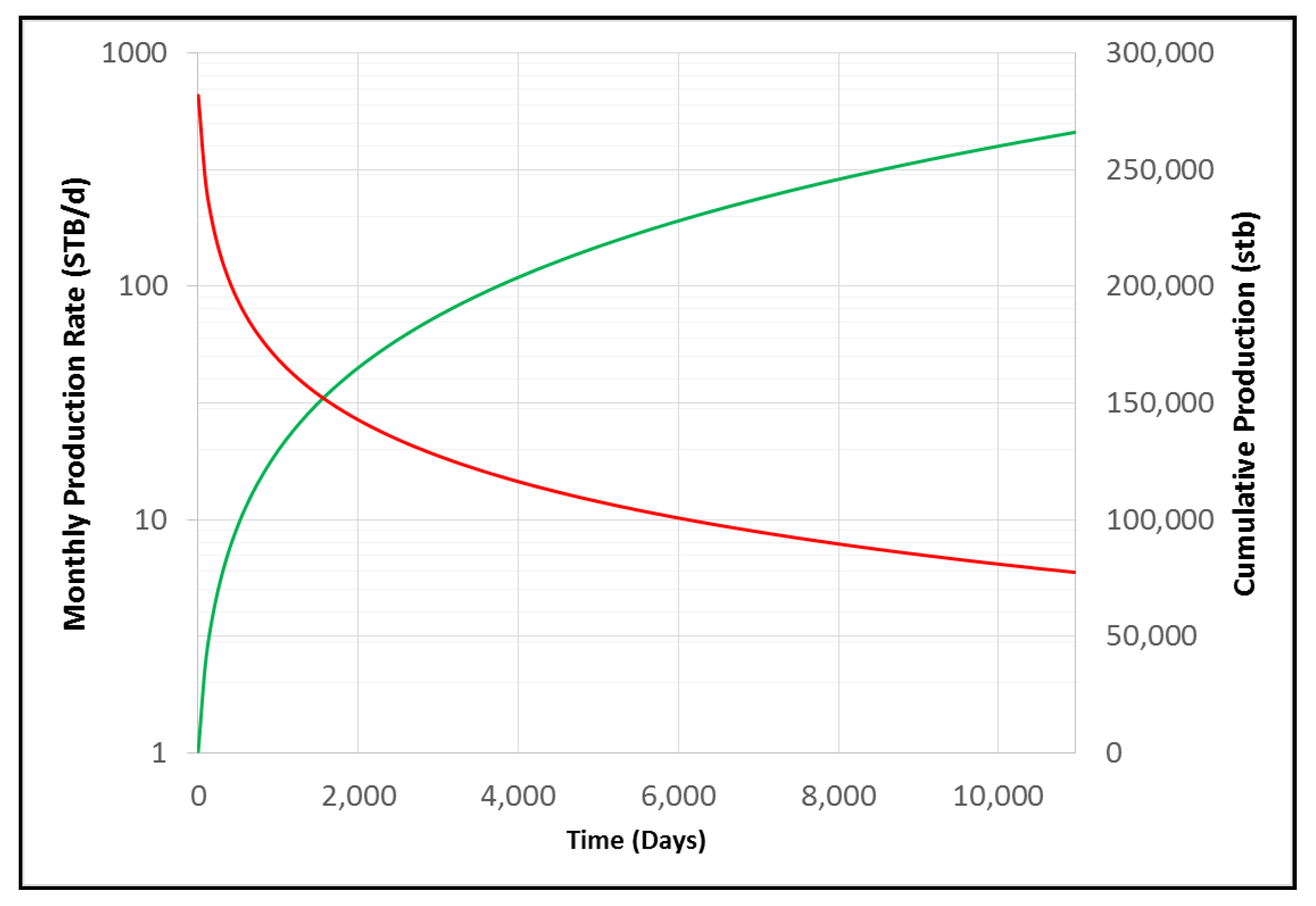
- Proper analysis of natural fracture data and the predominant mechanism by which it will affect flow will lead to accurate DRV calculations in the subsurface. From these determined DRV (based on a well type curve), fracture cluster spacing and well spacing could possibly be optimized.
Author Contributions
Funding
Conflicts of Interest
Nomenclature
| a | start of interval |
| b | end of interval |
| hk | natural fracture height [ft] |
| i | imaginary unit |
| kf | natural fracture permeability [nD] |
| km | matrix permeability [nD] |
| k (subscript) | summation index |
| m(t) | time dependent flow strength [ft2/month] |
| nf | fracture porosity |
| nm | matrix porosity |
| t | time [month] |
| vf | fluid velocity in natural fracture [ft/day] |
| vm | fluid velocity in matrix [ft/day] |
| wf | natural fracture aperture [ft] |
| z | complex coordinate |
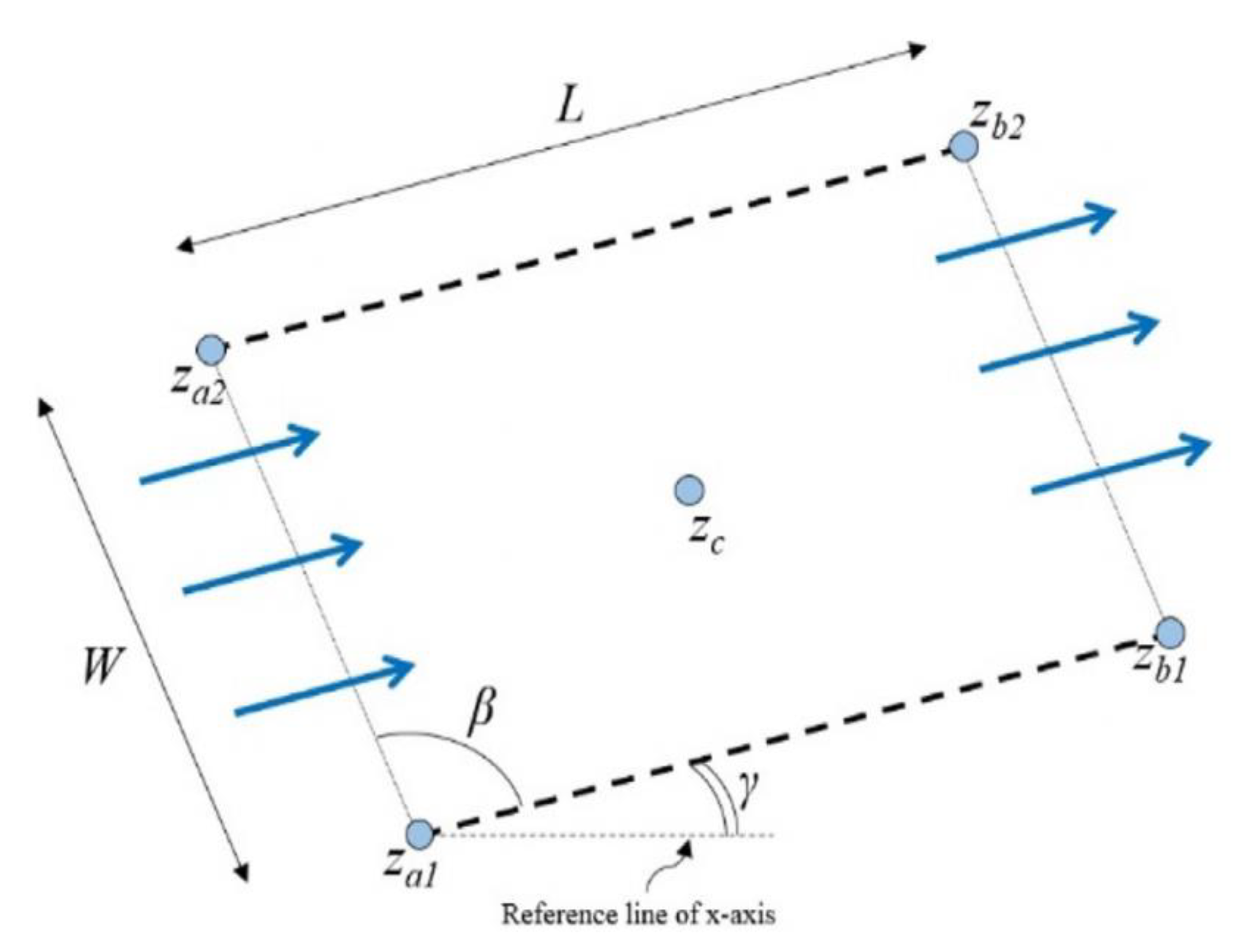
| za1 | corner point 1 of natural fracture domain |
| za2 | corner point 2 of natural fracture domain |
| zb1 | corner point 3 of natural fracture domain |
| zb2 | corner point 4 of natural fracture domain |
| zc | center of bounded natural fracture domain |
| Cf | fracture conductivity [mD.ft] |
| Hf | hydraulic fracture height [ft] |
| Lf | natural fracture length [ft] |
| P | pressure [psi] |
| Po | initial pressure [psi] |
| ∆P | pressure change [psi] |
| Rk | permeability ratio |
| Rn | porosity ratio |
| V | total velocity field in reservoir space [ft/day] |
| Ω | complex potential [ft2/day] |
| Φ | potential function |
| µ | fluid viscosity [cP] |
| β | angle between walls of natural fracture [degree] |
| γ | rotation angle of natural fracture to reference line along x-axis [degree] |
| υ | natural fracture flow strength [ft4/day] |
| Abbreviations | |
| CAM | complex analysis methods |
| CK | carman kozeny |
| DRV | drained rock volume |
| HFTS | hydraulic fracturing test site |
| REV | representative elementary volume |
| SRV | stimulated rock volume |
| TOF | time of flight |
| TOFC | time of flight contours |
| Conversion Factors from SI Units to Field Units | |
| 1 m | 3.28 ft |
| 1 Pa | 1.45 × 10⁻⁴ psi |
| 1 m2 | 1.01 × 10¹⁵ md |
| 1 m3/s | 5.434 × 10⁵ STB/day (oil) |
| 1 m3/s | 3049 Mscf/day (gas) |
| 1 Pa-s | 1000 cp |
Appendix A. Flux Modeling and Production Allocation for Hydraulic Line Sink Models

| Matrix Porosity (nm) | 0.05 |
| Matrix Permeability (km) | 100 nanoDarcy |
| Water-Oil Ratio (WOR) | 4.592 |
| Formation Volume Factor (B) | 1 |
| Viscosity (µ) | 1 centipoise |
| Residual Oil Saturation (Ro) | 0.20 |
| Hydraulic Fracture Height (H) | 60 ft |
| Hydraulic Fracture Length | 150 ft |

Appendix B. Carman–Kozeny Relation for Estimating Natural Fracture Permeability from Porosity
| Natural Fracture Porosity (%) | Natural Fracture Permeability (nD) | Rk | Matrix Velocity (ft/day) | Natural Fracture Width (ft) | Natural Fracture Length (ft) | Natural Fracture Height (ft) | Natural Fracture Strength (ft4/day) |
|---|---|---|---|---|---|---|---|
| 8.4 | 152.6 | 1.53 | 0.169 | 0.5 | 20 | 60 | 155 |
| 9.8 | 246.1 | 2.46 | 0.169 | 0.5 | 20 | 60 | 250 |
Appendix C. Upscaling for Fractured Porous Media


References
- Kresse, O.; Weng, X.; Gu, H.; Wu, R. Numerical Modeling of Hydraulic Fractures Interaction in Complex Naturally Fractured Formations. Rock Mech. Rock Eng. 2013, 46, 555–568. [Google Scholar] [CrossRef]
- Aguilera, R. Effect of Fracture Dip and Fracture Tortuosity on Petrophysical Evaluation of Naturally Fractured Reservoirs. Petrol. Soc. Canada 2008. [Google Scholar] [CrossRef]
- Tutuncu, A.; Bui, B.; Suppachoknirun, T. An Integrated Study for Hydraulic Fracture and Natural Fracture Interactions and Refracturing in Shale Reservoirs Hydraulic Fracture Modeling; Gulf Professional Publishing: Oxford, UK, 2018; pp. 323–348. [Google Scholar] [CrossRef]
- Weijermars, R.; Van Harmelen, A. Breakdown of doublet recirculation and direct line drives by far-field flow in reservoirs: Implications for geothermal and hydrocarbon well placement. Geophys. J. Int. 2016, 206, 19–47. [Google Scholar] [CrossRef]
- Doe, T.; Lacazette, A.; Dershowitz, W.; Knitter, C. Evaluating the Effect of Natural Fractures on Production from Hydraulically Fractured Wells Using Discrete Fracture Network Models. In Proceedings of the Unconventional Resources Technology Conference, Denver, CO, USA, 12–14 August 2013; pp. 1679–1688. [Google Scholar]
- Olson, J.E.; Taleghani, A.D. Modeling simultaneous growth of multiple hydraulic fractures and their interaction with natural fractures. In Proceedings of the SPE Hydraulic Fracturing Technology Conference, Woodlands, TX, USA, 19–21 January 2009. [Google Scholar]
- Cipolla, C.L.; Warpinski, N.R.; Mayerhofer, M.J.; Lolon, E.; Vincent, M.C. The Relationship Between Fracture Complexity, Reservoir Properties, and Fracture Treatment Design. Soc. Pet. Eng. 2008. [Google Scholar] [CrossRef]
- Warpinski, N.R.; Moschovidis, Z.A.; Parker, C.D.; Abou-Sayed, I.S. Comparison study of hydraulic fracturing models—Test case: GRI staged field Experiment No. 3 (includes associated paper 28158). SPE Prod. Facil. 1994, 9, 7–16. [Google Scholar] [CrossRef]
- Parsegov, S.G.; Nandlal, K.; Schechter, D.S.; Weijermars, R. Physics-Driven Optimization of Drained Rock Volume for Multistage Fracturing: Field Example from the Wolfcamp Formation, Midland Basin. In Proceedings of the Unconventional Resources Technology Conference, Houston, TX, USA, 23–25 July 2018. [Google Scholar]
- Popovici, A.M.; Fomel, S.; Grechka, V.; Li, Z.; Howell, R.; Vavrycuk, V. Single-well moment tensor inversion of tensile microseismic events. SEG Tech. Program Expand. Abstr. 2017, 81, 2746–2751. [Google Scholar]
- Raterman, K.T.; Farrell, H.E.; Mora, O.S.; Janssen, A.L.; Gomez, G.A.; Busetti, S.; Warren, M. Sampling a Stimulated Rock Volume: An Eagle Ford Example. In Proceedings of the Unconventional Resources Technology Conference, Austin, TX, USA, 24–26 July 2017. [Google Scholar] [CrossRef]
- Shrivastava, K.; Hwang, J.; Sharma, M. Formation of Complex Fracture Networks in the Wolfcamp Shale: Calibrating Model Predictions with Core Measurements from the Hydraulic Fracturing Test Site. Soc. Pet. Eng. 2018. [Google Scholar] [CrossRef]
- Fisher, M.; Wright, C.; Davidson, B.; Goodwin, A.; Fielder, E.; Buckler, W.; Steinsberger, N. Integrating Fracture Mapping Technologies to Optimize Stimulations in the Barnett Shale. SPE Annu. Tech. Conf. Exhib. 2005, 20, 85–93. [Google Scholar]
- Maxwell, S.; Urbancic, T.; Steinsberger, N.; Zinno, R. Microseismic Imaging of Hydraulic Fracture Complexity in the Barnett Shale. In Proceedings of the SPE Annual Technical Conference and Exhibition, San Antonio, TX, USA, 29 September–2 October 2002. [Google Scholar]
- Pradhan, V.R.; Meert, J.G.; Pandit, M.K.; Kamenov, G.; Mondal, M.E.A. Paleomagnetic and geochronological studies of the mafic dyke swarms of Bundelkhand craton, central India: Implications for the tectonic evolution and paleogeographic reconstructions. Precambrian Res. 2012, 198, 51–76. [Google Scholar] [CrossRef]
- Kilaru, S.; Goud, B.K.; Rao, V.K. Crustal structure of the western Indian shield: Model based on regional gravity and magnetic data. Geosci. Front. 2013, 4, 717–728. [Google Scholar] [CrossRef] [Green Version]
- McKenzie, N.R.; Hughes, N.C.; Myrow, P.M.; Banerjee, D.M.; Deb, M.; Planavsky, N.J. New age constraints for the Proterozoic Aravalli–Delhi successions of India and their implications. Precambrian Res. 2013, 238, 120–128. [Google Scholar] [CrossRef]
- Huang, J.I.; Kim, K. Fracture process zone development during hydraulic fracturing. Int. J. Rock Mech. Min. Sci. Geéomeéch. Abstr. 1993, 30, 1295–1298. [Google Scholar] [CrossRef]
- Weijermars, R.; Van Harmelen, A.; Zuo, L.; Nascentes, I.A.; Yu, W. High-Resolution Visualization of Flow Interference Between Frac Clusters (Part 1): Model Verification and Basic Cases. In Proceedings of the Unconventional Resources Technology Conference, Austin, TX, USA, 24–26 July 2017. [Google Scholar]
- Weijermars, R.; Van Harmelen, A.; Zuo, L. Flow Interference Between Frac Clusters (Part 2): Field Example from the Midland Basin (Wolfcamp Formation, Spraberry Trend Field) With Implications for Hydraulic Fracture Design. In Proceedings of the Unconventional Resources Technology Conference, Austin, TX, USA, 24–26 July 2017. [Google Scholar]
- Nandlal, K.; Weijermars, R. Drained rock volume around hydraulic fractures in porous media: Planar fractures versus fractal networks. Pet. Sci. 2019, 1–22. [Google Scholar] [CrossRef]
- Van Harmelen, A.; Weijermars, R. Complex analytical solutions for flow in hydraulically fractured hydrocarbon reservoirs with and without natural fractures. Appl. Math. Model. 2018, 56, 137–157. [Google Scholar] [CrossRef]
- Weijermars, R.; Khanal, A. High-resolution streamline models of flow in fractured porous media using discrete fractures: Implications for upscaling of permeability anisotropy. Earth-Science Rev. 2019, 194, 399–448. [Google Scholar] [CrossRef]
- Forand, D.; Heesakkers, V.; Schwartz, K. Constraints on Natural Fracture and In-situ Stress Trends of Unconventional Reservoirs in the Permian Basin, USA. In Proceedings of the Unconventional Resources Technology Conference, Austin, TX, USA, 24–26 July 2017. [Google Scholar] [CrossRef]
- Gale, J.F.; Laubach, S.E.; Olson, J.E.; Eichhuble, P.; Fall, A. Natural Fractures in shale: A review and new observations. AAPG Bull. 2014, 98, 2165–2216. [Google Scholar] [CrossRef]
- Gutierrez, M.; Øino, L.; Nygard, R. Stress-dependent permeability of a de-mineralised fracture in shale. Mar. Pet. Geol. 2000, 17, 895–907. [Google Scholar] [CrossRef]
- Laubach, S.E. Practical approaches to identifying sealed and open fractures. AAPG Bull. 2003, 87, 561–579. [Google Scholar] [CrossRef]
- Zuo, L.; Weijermars, R. Rules for flight paths and time of flight for flows in heterogeneous isotropic and anisotropic porous media. Geofluids 2017. [Google Scholar] [CrossRef]
- Warren, J.; Root, P. The Behavior of Naturally Fractured Reservoirs. Soc. Pet. Eng. J. 1963, 3, 245–255. [Google Scholar] [CrossRef] [Green Version]
- Kazemi, H.; Merrill, L.S.; Porterfield, K.L.; Zeman, P.R. December 1. Numerical Simulation of Water-Oil Flow in Naturally Fractured Reservoirs. Soc. Pet. Eng. 1976. [Google Scholar] [CrossRef]
- Huang, T.; Guo, X.; Chen, F. Modeling transient flow behavior of a multiscale triple porosity model for shale gas reservoirs. J. Nat. Gas Sci. Eng. 2015, 23, 33–46. [Google Scholar] [CrossRef]
- Sang, G.; Elsworth, D.; Miao, X.; Mao, X.; Wang, J. Numerical study of a stress dependent triple porosity model for shale gas reservoirs accommodating gas diffusion in kerogen. J. Nat. Gas Sci. Eng. 2016, 32, 423–438. [Google Scholar] [CrossRef]
- Weijermars, R.; Van Harmelen, A. Shale Reservoir Drainage Visualized for a Wolfcamp Well (Midland Basin, West Texas, USA). Energies 2018, 11, 1665. [Google Scholar] [CrossRef]
- Long, J.C.S.; Remer, J.S.; Wilson, C.R.; Witherspoon, P.A. Porous media equivalents for networks of discontinuous fractures. Water Resour. Res. 1982, 18, 645–658. [Google Scholar] [CrossRef] [Green Version]
- Rogers, S.; Elmo, D.; Dunphy, R.; Bearinger, D. Understanding Hydraulic Fracture Geometry and Interactions in the Horn River Basin Through DFN and Numerical Modeling. In Proceedings of the Canadian Unconventional Resources and International Petroleum Conference, Calgary, AB, Canada, 19–21 October 2010. [Google Scholar]
- Dershowitz, W.S.; Ambrose, R.; Lim, D.H.; Cottrell, M.G. Hydraulic fracture and natural fracture simulation for improved shale gas development. In Proceedings of the American Association of Petroleum Geologists (AAPG) Annual Conference and Exhibition Houston, Houston, TX, USA, 10–13 April 2011. [Google Scholar]
- Jing, L.; Stephansson, O. Fundamentals of Discrete Element Methods for Rock Engineering. Developments in Geotechnical Engineering; Elsevier: Amsterdam, The Netherlands, 2007; Volume 85. [Google Scholar] [CrossRef]
- Wu, K.; Olson, J.E. Numerical Investigation of Complex Hydraulic-Fracture Development in Naturally Fractured Reservoirs. Soc. Pet. Eng. 2016. [Google Scholar] [CrossRef]
- Nelson, R. Geological Analysis of Naturally Fractured Reservoirs, 2nd ed.; Gulf Professional Publishing: Oxford, UK, 2001. [Google Scholar]
- Tiab, D.; Restrepo, D.P.; Igbokoyi, A.O. Fracture Porosity of Naturally Fractured Reservoirs. Soc. Pet. Eng. 2006. [Google Scholar] [CrossRef]
- Zhang, X.; Thiercelin, M.J.; Jeffrey, R.G. Effects of Frictional Geological Discontinuities on Hydraulic Fracture Propagation. In Proceedings of the SPE Hydraulic Fracturing Technology Conference, College Station, TX, USA, 29–31 January 2007; pp. 29–31. [Google Scholar]
- Soeder, D. Porosity and Permeability of Eastern Devonian Gas Shale. SPE Form. Eval. 1988, 3, 116–124. [Google Scholar] [CrossRef]
- Gale, J.F.W.; Reed, R.M.; Holder, J. Natural fractures in the Barnett Shale and their importance for hydraulic fracture treatments. AAPG Bull. 2007, 91, 603–622. [Google Scholar] [CrossRef]
- Nelson, R.A. Geologic Analysis of Naturally Fractured Reservoirs; Gulf Publishing: Houston, TX, USA, 1985; p. 320. [Google Scholar]
- Weber, K.J.; Bakker, M. Fracture and vuggy porosity. In Proceedings of the Society of Petroleum Engineers 56th Annual Fall Technical Conference, San Antonio, TX, USA, 5–7 October 1981; p. 11. [Google Scholar]
- Lee, D.S.; Herman, J.D.; Elsworth, D.; Kim, H.T.; Lee, H.S. A critical evaluation of unconventional gas recovery from the marcellus shale, northeastern United States. KSCE J. Civ. Eng. 2011, 15, 679–687. [Google Scholar] [CrossRef]
- Muskat, M. The Theory of Potentiometric Models. Trans. AIME 1949, 179, 216–221. [Google Scholar] [CrossRef]
- Strack, O.D.L. Groundwater Mechanics; Prentice-Hall: Englewood Cliffs, NJ, USA, 1989. [Google Scholar]
- Sato, K. Complex Analysis for Practical Engineering; Springer Science and Business Media LLC: Berlin/Heidelberg, Germany, 2015. [Google Scholar]
- Weijermars, R. Visualization of space competition and plume formation with complex potentials for multiple source flows: Some examples and novel application to Chao lava flow (Chile). J. Geophys. Res. Solid Earth 2014, 119, 2397–2414. [Google Scholar] [CrossRef] [Green Version]
- Weijermars, R.; Dooley, T.P.; Jackson, M.P.A.; Hudec, M.R. Rankine models for time-dependent gravity spreading of terrestrial source flows over subplanar slopes. J. Geophys. Res. Solid Earth 2014, 119, 7353–7388. [Google Scholar] [CrossRef] [Green Version]
- Weijermars, R.; Van Harmelen, A.; Zuo, L. Controlling flood displacement fronts using a parallel analytical streamline simulator. J. Pet. Sci. Eng. 2016, 139, 23–42. [Google Scholar] [CrossRef]
- Potter, H.D.P. On Conformal Mappings and Vector Fields. Senior Thesis, Marietta College, Marietta, OH, USA, 2008. [Google Scholar]
- Wu, K.; Olson, J.E. Mechanics Analysis of Interaction Between Hydraulic and Natural Fractures in Shale Reservoirs. In Proceedings of the Unconventional Resources Technology Conference, Denver, CO, USA, 25–27 August 2014. [Google Scholar] [CrossRef]
- Taleghani, A.D.; Olson, J.E. How Natural Fractures Could Affect Hydraulic-Fracture Geometry. SPE J. 2013, 19, 161–171. [Google Scholar] [CrossRef]
- Kumar, A.; Shrivastava, K.; Manchanda, R.; Sharma, M. An Efficient Method for Modeling Discrete Fracture Networks in Geomechanical Reservoir Simulation. In Proceedings of the Unconventional Resources Technology Conference, Denver, CO, USA, 25 July 2019. [Google Scholar] [CrossRef]
- Gale, J.F.W.; Elliott, S.J.; Laubach, S.E. Hydraulic Fractures in Core from Stimulated Reservoirs: Core Fracture Description of HFTS Slant Core. In Proceedings of the Unconventional Resources Technology Conference, Midland Basin, TX, USA, 9 August 2018. [Google Scholar] [CrossRef]
- Khanal, A.; Nandlal, K.; Weijermars, R. Impact of Natural Fractures on the Shape and Location of Drained Rock Volumes in Unconventional Reservoirs: Case Studies from the Permian Basin. In Proceedings of the Unconventional Resources Technology Conference, Austin, TX, USA, 31 July 2019. [Google Scholar] [CrossRef]
- Khanal, A.; Weijermars, R. Modeling Flow and Pressure Fields in Porous Media with High Conductivity Flow Channels and Smart Placement of Branch Cuts for Variant and Invariant Complex Potentials. Fluids 2019, 4, 154. [Google Scholar] [CrossRef]
- Khanal, A.; Weijermars, R. Pressure depletion and drained rock volume near hydraulically fractured parent and child wells. J. Pet Sci. Eng. 2019, 172, 607–626. [Google Scholar] [CrossRef]
- Weijermars, R.; Nandlal, K.; Khanal, A.; Tugan, M.F. Comparison of pressure front with tracer front advance and principal flow regimes in hydraulically fractured wells in unconventional reservoirs. J. Pet. Sci. Eng. 2019, 183, 106407. [Google Scholar] [CrossRef]
- Duda, A.; Koza, Z.; Matyka, M. Hydraulic tortuosity in arbitrary porous media flow. Phys. Rev. E 2011, 84, 036319. [Google Scholar] [CrossRef] [Green Version]
- Ma, J. Review of permeability evolution model for fractured porous media. J. Rock Mech. Geotech. Eng. 2015, 7, 351–357. [Google Scholar] [CrossRef] [Green Version]
- Tinni, A.; Sondergeld, C.; Rai, C. Particle size effect on porosity and specific surface area measurements of shales. In Proceedings of the International Symposium of the Society of Core Analysts, Avignon, France, 8–11 September 2014. [Google Scholar]
- U.S. Energy Information Administration (EIA). Permian Basin, Wolfcamp Shale Play, Geology Review; U.S. Energy Information Administration: Washington, DC, USA, 2018.
- Chen, T.; Clauser, C.; Marquart, G.; Willbrand, K.; Mottaghy, D. A new upscaling method for fractured porous media. Adv. Water Resour. 2015, 80, 60–68. [Google Scholar] [CrossRef]
- Chen, T.; Clauser, C.; Marquart, G.; Willbrand, K.; Büsing, H. Modeling anisotropic flow and heat transport by using mimetic finite differences. Adv. Water Resour. 2016, 94, 441–456. [Google Scholar] [CrossRef]


| Figure Number | Natural Fracture Strength (ft4/year) | Natural Fracture Length (ft) | Natural Fracture Width (ft) | Natural Fracture Height (ft) | Matrix Flow Rate (ft/year) | Permeability Ratio (Rk) | Natural Fracture Permeability (nD) | |
|---|---|---|---|---|---|---|---|---|
| 5 | NF1 | 0.1 | 25 | 5 | 1 | 2.5 | - a | - a |
| NF2 | 40 | 25 | 5 | 1 | 2.5 | 0.13 | 12.8 a | |
| NF3 | 160 | 25 | 5 | 1 | 2.5 | 0.51 | 51.2 a | |
| NF4 | 500 | 25 | 5 | 1 | 2.5 | 1.60 | 160 | |
| NF5 | 1000 | 25 | 5 | 1 | 2.5 | 3.20 | 320 | |
| 6b | 1000 | 25 | 5 | 1 | 2.5 | 3.20 | 320 | |
| 7 | 500 | 25 | 5 | 1 | 2.5 | 1.60 | 160 | |
| (ft4/day) | (ft/day) | |||||||
| 9 | a | 2500 | 20 | 10 | 60 | 0.1693 | 1.23 | 123.06 |
| b | 5000 | 20 | 10 | 60 | 0.1693 | 2.46 | 246.11 | |
| c | 10,000 | 20 | 10 | 60 | 0.1693 | 4.92 | 492.22 | |
| 10 | 5000 | 20 | 10 | 60 | 0.1693 | 2.46 | 246.11 | |
| 11b | 155 | 20 | 0.5 | 60 | 0.1693 | 1.53 | 152.59 | |
| 12 | 155 | 30 | 0.5 | 60 | 0.1693 | 1.02 | 101.73 | |
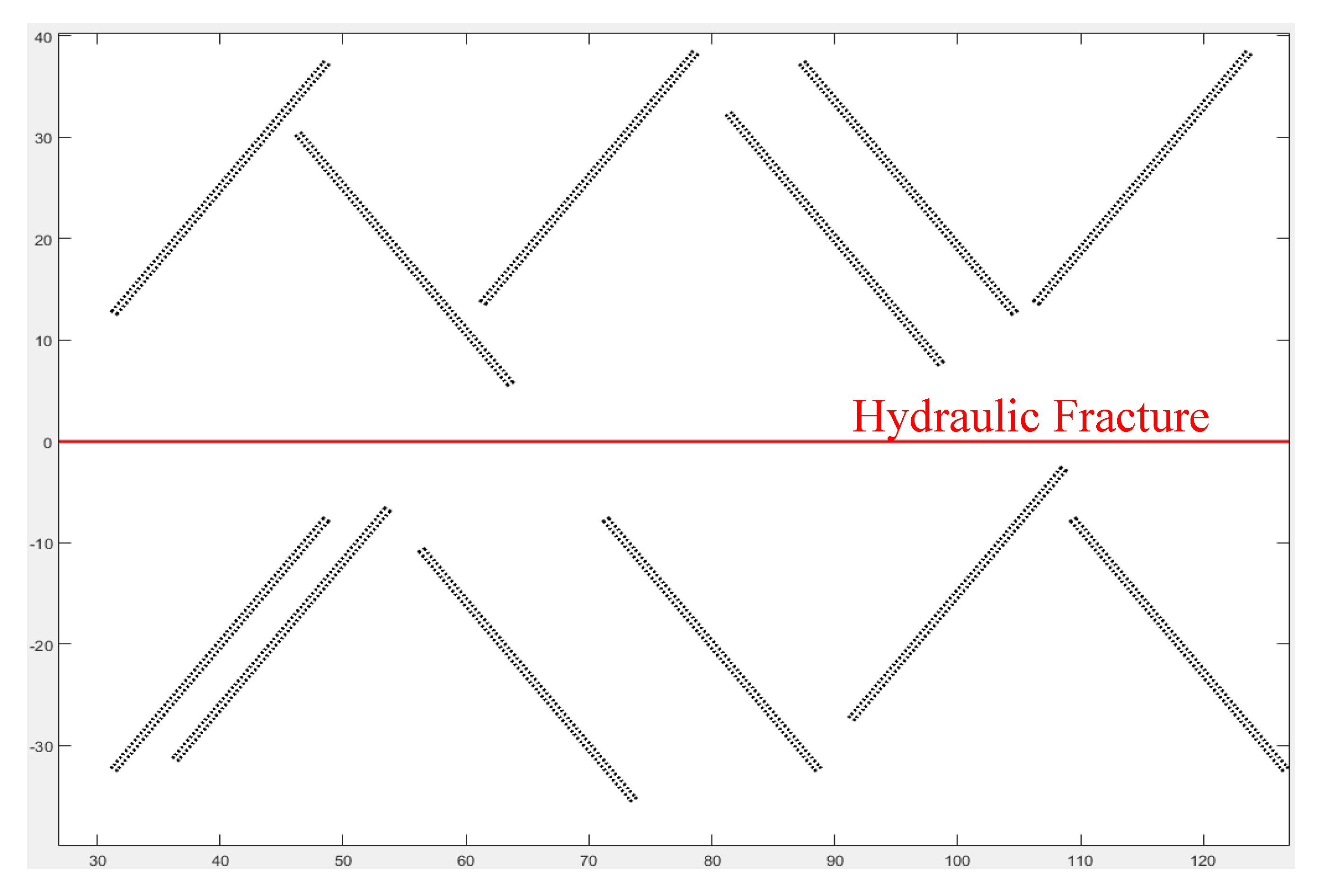
| Natural fracture orientation (to hydraulic fracture) a | −55° and 55° |
| Natural fracture length b | 30 ft |
| Original natural fracture density c | 0.042 fractures/ft2 |
| Assumed original natural fracture aperture | 0.2 inches |
| Upscaled natural fracture aperture d | 6 inches |
| Number of natural fractures d | 12 |
| Natural fracture porosity | 7.32% |
| Natural fracture strength | 155 ft4/day |
© 2019 by the authors. Licensee MDPI, Basel, Switzerland. This article is an open access article distributed under the terms and conditions of the Creative Commons Attribution (CC BY) license (http://creativecommons.org/licenses/by/4.0/).
Share and Cite
Nandlal, K.; Weijermars, R. Impact on Drained Rock Volume (DRV) of Storativity and Enhanced Permeability in Naturally Fractured Reservoirs: Upscaled Field Case from Hydraulic Fracturing Test Site (HFTS), Wolfcamp Formation, Midland Basin, West Texas. Energies 2019, 12, 3852. https://doi.org/10.3390/en12203852
Nandlal K, Weijermars R. Impact on Drained Rock Volume (DRV) of Storativity and Enhanced Permeability in Naturally Fractured Reservoirs: Upscaled Field Case from Hydraulic Fracturing Test Site (HFTS), Wolfcamp Formation, Midland Basin, West Texas. Energies. 2019; 12(20):3852. https://doi.org/10.3390/en12203852
Chicago/Turabian StyleNandlal, Kiran, and Ruud Weijermars. 2019. "Impact on Drained Rock Volume (DRV) of Storativity and Enhanced Permeability in Naturally Fractured Reservoirs: Upscaled Field Case from Hydraulic Fracturing Test Site (HFTS), Wolfcamp Formation, Midland Basin, West Texas" Energies 12, no. 20: 3852. https://doi.org/10.3390/en12203852