Behaviour of Distribution Grids with the Highest PV Share Using the Volt/Var Control Chain Strategy

Abstract

The large-scale integration of rooftop PVs stalls due to the voltage limit violations they provoke, the uncontrolled reactive power flow in the superordinate grids and the information and communications technology (ICT) related challenges that arise in solving the voltage limit violation problem. This paper attempts to solve these issues using the LINK-based holistic architecture, which takes into account the behaviour of the entire power system, including customer plants. It focuses on the analysis of the behaviour of distribution grids with the highest PV share, leading to the determination of the structure of the Volt/var control chain. The voltage limit violations in low voltage grid and the ICT challenge are solved by using concentrated reactive devices at the end of low voltage feeders. Q-Autarkic customer plants relieve grids from the load-related reactive power. The optimal arrangement of the compensation devices is determined by a series of simulations. They are conducted in a common model of medium and low voltage grids. Results show that the best performance is achieved by placing compensation devices at the secondary side of the supplying transformer. The Volt/var control chain consists of two Volt/var secondary controls; one at medium voltage level (which also controls the TSO-DSO reactive power exchange), the other at the customer plant level.

1. Introduction

Nowadays, climate change has become apparent, not only for scientists but also for everybody [1]. Reducing emissions through the use of renewable sustainable resources while maintaining a reliable and secure electricity supply is becoming increasingly imperative. In this context, the large-scale implementation of Distributed Generation (DG) holds a considerable potential [2].

European utilities supply 260 million customers, of which more than 99% are connected at the Low Voltage (LV) level [3]. The use of inverters available in DGs, e.g., rooftop photovoltaic (PV), to control the voltage in distribution networks [4] has introduced various local control strategies such as cos $\phi$ (P), Q(U), and so on [5,6,7] that provoke uncontrolled reactive power flows on the superordinate grids. Implementing PVs on the rooftop of each customer requires the coordination of millions of local controllers needed to operate the power system reliably and securely. A flood of data exchange is necessary that poses serious challenges to ICT, cyber security and data privacy [8,9,10].

The optimal volt/var management or control is one of the most essential processes for utilities to maintain reliable voltages and to keep the power factor close to one. Currently, they use reactive devices (RDs) to reduce the amount of reactive power flowing through transmission lines and to maintain sufficient reactive power capability in transmission systems [11]. In medium voltage (MV) grids, capacitor banks are mostly used to support the voltage [12]. The uncontrolled reactive power flow in high voltage (HV) and MV levels provoked by the large scale implementation of local control strategies in LV level upsets the current practices [13]. In the process of reactive power management are already involved different actors, i.e., transmission (TSO) and distribution system operators (DSO) and customers (as owners of PV inverters). Considering the perspective of individual actors or optimizing individual functionalities may lead to suboptimal solutions and other, difficult to overcome, challenges. In contrast, the holistic architecture vision enables large-scale rollout of the new control paradigms leading to optimal solutions [14]. Volt/var control chain strategy promises the solution of the problem related to voltage control and reactive power management that is of utmost importance to utilities, as they may favor the large scale integration of distributed generation.

The volt/var control chain strategy that comprises all grid levels, i.e., HV, MV, LV and Customer Plant (CP) grid, located on the vertical axis (Y-axis) of the holistic model “The energy supply chain net” [15] is introduced in [16]. It relies on the LINK-based holistic architecture [17], where the Secondary Control (SC) is the crucial instrument to realize a sustainable and reliable grid operation of the whole power system including CPs. The implementation of secondary control in CP level enables the full reactive power (Q) compensation of the customer plants, leading to Q-self-sufficient or Q-Autarkic customers [18]. The DSO owned reactive devices, e.g., L(U)-controlled coils, installed at LV feeders with voltage limit violation potential, keep the voltage within the limits [19], while providing substantial technical (reduced losses, Q-exchange and Distribution Transformer (DTR) loading [20]; and increased hosting capacity [21]) and social (preserved data privacy and avoided discrimination [20]) benefits compared to the cos $\phi$ (P)- and Q(U)-control strategies. Further on, the L(U)+Q-Autarky control ensemble provides substantial technical benefits compared to the L(U)-control strategy [18].

All var-local control strategies, i.e., cos$\phi$ (P), Q(U), L(U), etc., provoke uncontrolled reactive power flows in the superordinate voltage level grids inclusive the HV grid. The reactive power margin (RPM) decreases significantly if the DG production comes close to the demand or even exceeds it [22]. The power system approaches a voltage instable situation.

This paper examines the effect of additional compensation devices (CDs) on the distribution grid behaviour, when the volt/var control chain strategy that implies the L(U)+Q-autarky control ensemble is used. Furthermore, the optimal link-grid size is investigated for the specific conditions.

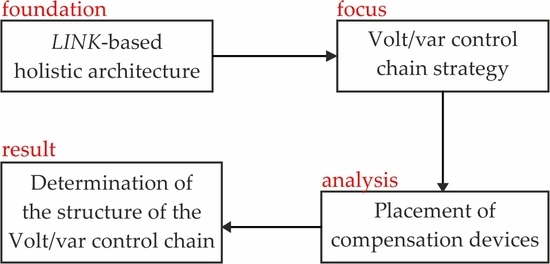
Section 2 gives an overview of the fundamentals of the volt/var control chain strategy, the description of the customer plant and distribution grid model, and the definition of the simulated control setups. Section 3 presents the investigation results concerning the distribution grid behaviour and the effect of CD placement. Furthermore, a grid-link setup for practical implementation is presented. Finally, in Section 4, some concluding remarks are summarized.

2. Materials and Methods

This work builds on the LINK-based holistic architecture and the associated strategy of volt/var control chain, the fundamentals of which are outlined below. After that follows the model description of the considered grids and of the simulated control setups.

2.1. Fundamentals of Volt/Var Control Chain Strategy

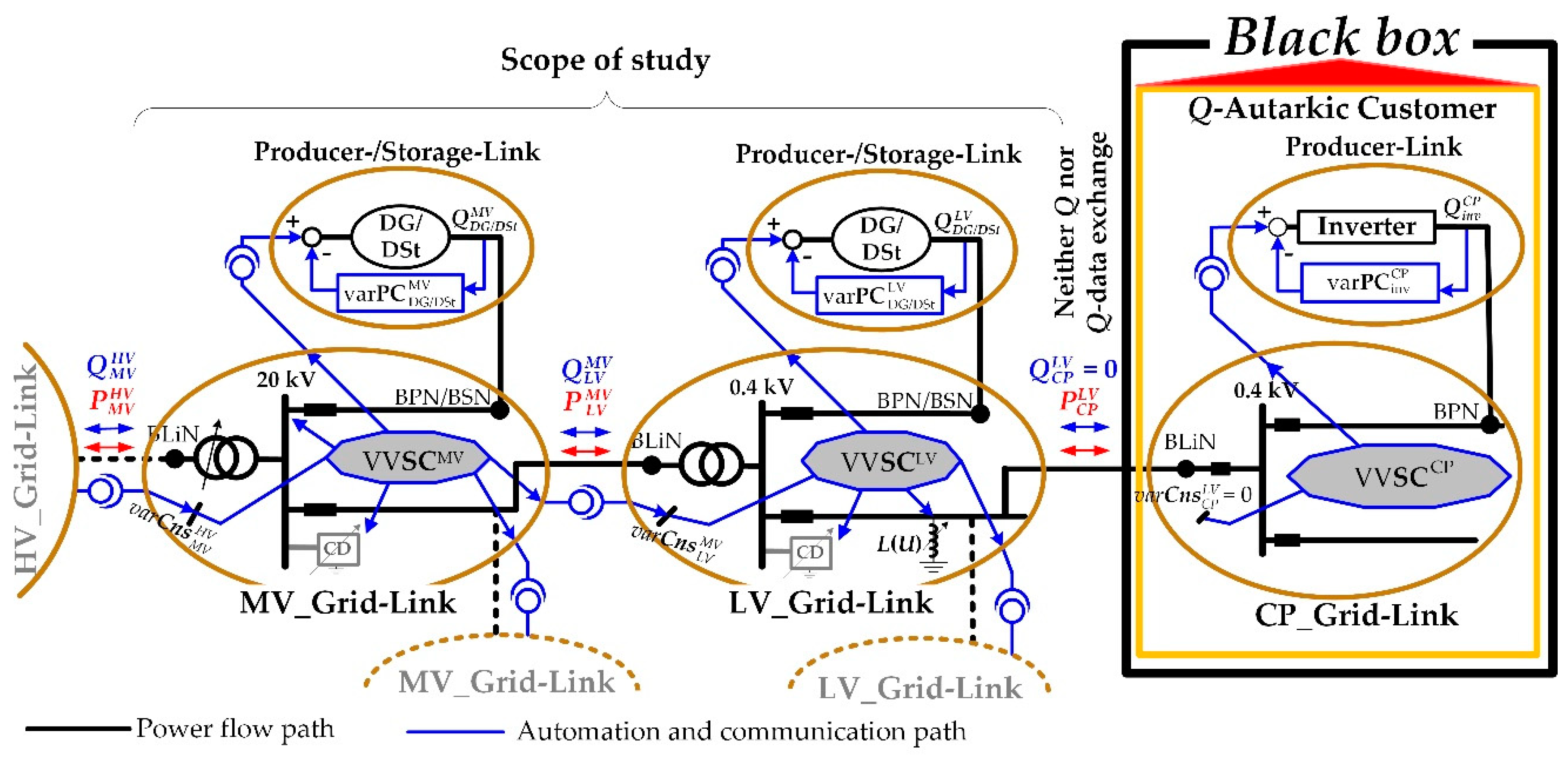
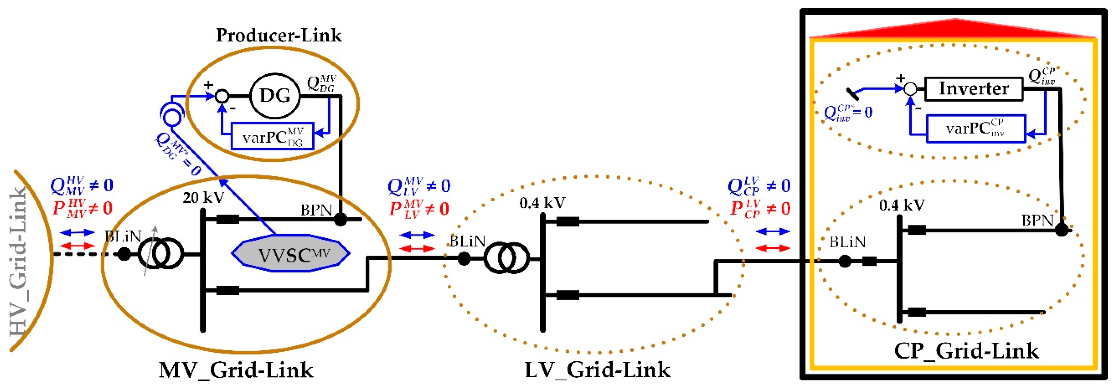
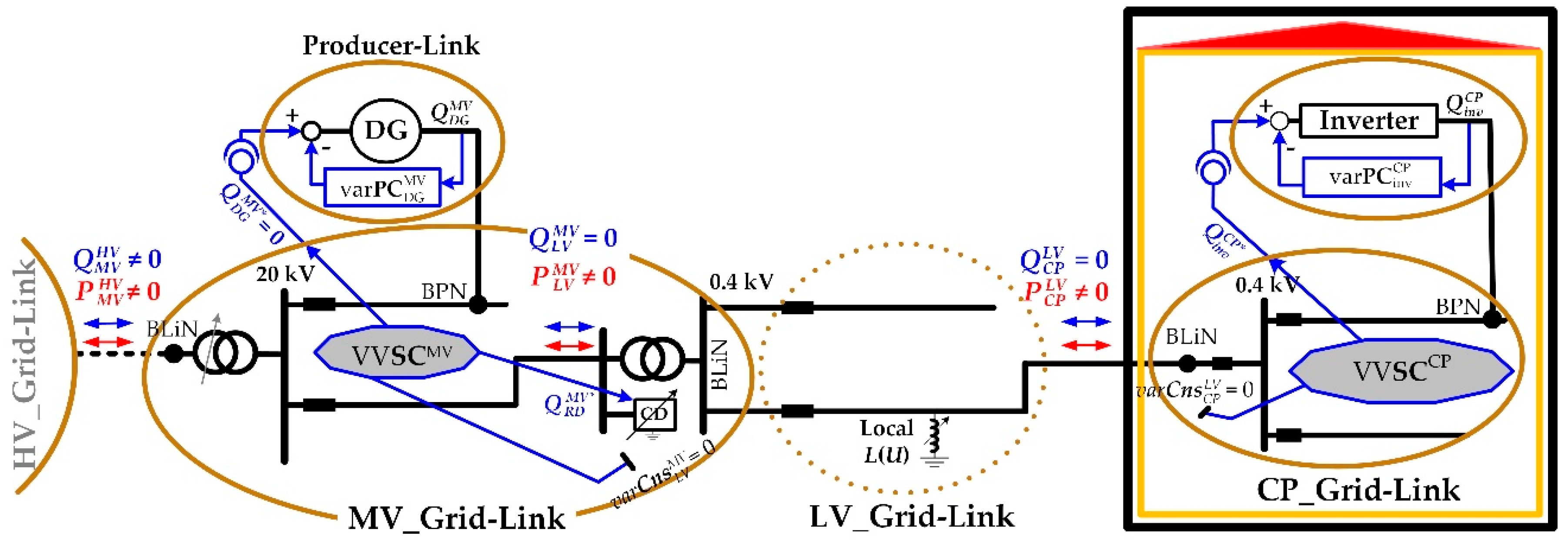
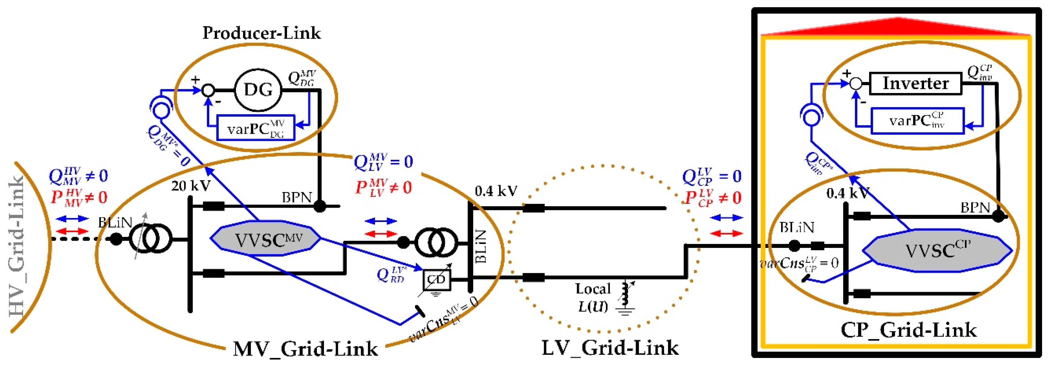
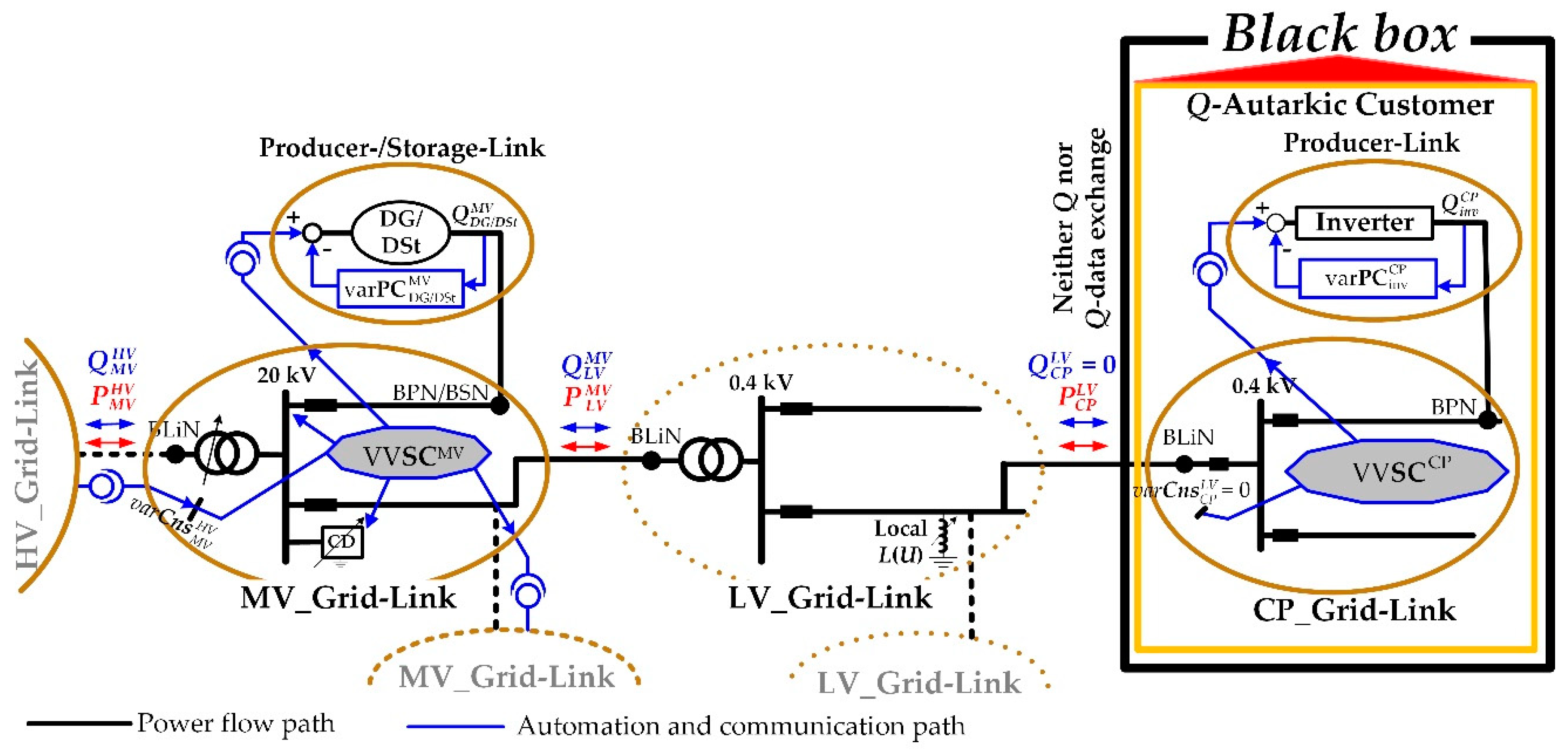
SC is the base instrument to realize the volt/var control chain strategy. It is one of the fundamental components of each grid-link [17]. It refers to control actions that are calculated based on the grid-link control area. It fulfils a predefined objective function by respecting the dynamic grid constraints on the grid-link boundaries and the static constraints of electrical appliances (PQ-diagrams of generators, transformer rating, etc.). Dynamic grid constraints are the reactive and active power exchange at the grid-link boundaries that are agreed from the corresponding grid-link operators. The grid-link contains SC-loops for both major entities of power systems—frequency and voltage. This paper deals with the volt/var secondary control (VVSC) schemas. The generalized form of volt/var control chain strategy [16] in the Y-axis of the holistic model “The energy supply chain net” that implies the L(U)+Q-autarky control ensemble [18] is shown in Figure 1. All relevant links are drawn in gold-coloured solid lines, while the neighbour grid-links are indicated by gold-dashed lines. Grid-links are set upon three classical levels: CP, LV and MV level. The automation and communication path is blue, while the power flow path is black.

RDs are used in power systems for two purposes: for voltage control (voltage control reactive device—VCRD) or reactive power compensation (compensation device—CD). The corresponding varPCs receive the set-points U* and Q* as in

Table 1. Devices considered for voltage-control and var-compensation.

Device		Purpose	Set-Point for varPC
RD	VCRD	Voltage control	U*
	CD	Var compensation	Q*

.

The main reason to introduce inductive devices on the low voltage grid is to keep the voltage within the limits over the all-time horizon. L(U)s are VCRD, e.g., coils, connected at the end of LV feeders, which may violate the upper voltage limit. The positioning of L(U)s at the LV feeder end shows high effectiveness due to the prevalent high voltage sensitivity ($\partial \mathrm{U}/\partial \mathrm{Q}$) [23]. Q-autarky is a special mode of operation of the volt/var secondary control set up in the CP level (${\mathrm{VV}\mathbf{SC}}^{\mathrm{CP}}$). Neither Q ($Q_{CP}^{LV}=0$) nor Q-data exchange with the LV grid is required when operating the distribution grid with high PV-share. CPs are Q-self-sufficient.

The following generalized equation is introduced for the first time to compactly represent the VVC chain in the Y-axis:

$$\begin{array}{c}{\mathrm{VVC}}^{\mathrm{Y}-\mathrm{axis}}{=\{\mathrm{VV}\mathbf{SC}}^{\mathrm{MV}}\left({\mathrm{volt}\mathbf{PC}}_{\mathrm{OLTC}}^{\mathrm{MV}}{,\mathrm{var}\mathbf{PC}}_{\mathrm{RD}}^{\mathrm{MV}}{,\mathrm{var}\mathbf{PC}}_{\mathrm{DG}/\mathrm{DSt}}^{\mathrm{MV}}{,\mathrm{VV}\mathbf{SC}}_{\mathrm{ngb}}^{\mathrm{MV},\mathrm{LV}}{,\mathrm{var}\mathbf{Cns}}_{\mathrm{MV}}^{\mathrm{HV}}\right),\hfill \\ {\mathrm{VV}\mathbf{SC}}^{\mathrm{LV}}\left({\mathrm{var}\mathbf{PC}}_{\mathrm{RD}}^{\mathrm{LV}}{,\mathrm{var}\mathbf{PC}}_{\mathrm{DG}/\mathrm{DSt}}^{\mathrm{LV}}{,\mathrm{VV}\mathbf{SC}}_{\mathrm{ngb}}^{\mathrm{LV},\mathrm{CP}}{,\mathrm{var}\mathbf{Cns}}_{\mathrm{LV}}^{\mathrm{MV}}\right){,\mathrm{VV}\mathbf{SC}}^{\mathrm{CP}}\left({\mathrm{var}\mathbf{PC}}_{\mathrm{inv}}^{\mathrm{CP}}{,\mathrm{var}\mathbf{Cns}}_{\mathrm{CP}}^{\mathrm{LV}}=0\right)\}\hfill \end{array}$$

(1)

where ${\mathrm{VV}\mathbf{SC}}^{\mathrm{MV}}$ calculates in real time

(a)

the voltage set-point for the primary control ${\mathrm{volt}\mathbf{PC}}_{\mathrm{OLTC}}^{\mathrm{MV}}$ of the supplying transformer and other transformers included in the MV_link-grid (e.g., 34.5 kV/11 kV, etc.) that have On-Load-Tap-Changer (OLTC);

(b)

the var set-points for the primary controls ${\mathrm{var}\mathbf{PC}}_{\mathrm{RD}}^{\mathrm{MV}}$ of all RDs included in the MV_link-grid;

(c)

the var set-points for the primary controls ${\mathrm{var}\mathbf{PC}}_{\mathrm{DG}/\mathrm{DSt}}^{\mathrm{MV}}$ of all DGs and Distributed Storages (DSt) connected to the MV_link-grid;

(d)

the var set-points for the Volt/var secondary controls ${\mathrm{VV}\mathbf{SC}}_{\mathrm{ngb}}^{\mathrm{MV},\mathrm{LV}}$ of all neighbour MV_ or LV_grid-links, while respecting the var constraint ${\mathrm{var}\mathbf{Cns}}_{\mathrm{MV}}^{\mathrm{HV}}$ at the border to the HV_link-grid.

${\mathrm{VV}\mathbf{SC}}^{\mathrm{LV}}$ calculates in real time:

(a)

the voltage and var set-points for the primary controls ${\mathrm{var}\mathbf{PC}}_{\mathrm{RD}}^{\mathrm{LV}}$ of all RDs included in the LV_link-grid;

(b)

the var set-points for the primary controls ${\mathrm{var}\mathbf{PC}}_{\mathrm{DG}/\mathrm{DSt}}^{\mathrm{LV}}$ of all DGs and DSts connected to the LV_link-grid;

(c)

the var set-points for the Volt/var secondary controls ${\mathrm{VV}\mathbf{SC}}_{\mathrm{ngb}}^{\mathrm{LV},\mathrm{CP}}$ of all neighbour LV_ or CP_grid-links, while respecting the var constraint ${\mathrm{var}\mathbf{Cns}}_{\mathrm{LV}}^{\mathrm{MV}}$ at the border to the MV_link-grid.

(d)

${\mathrm{VV}\mathbf{SC}}^{\mathrm{CP}}$ calculates in real time

(e)

the var set-point for the primary control ${\mathrm{var}\mathbf{PC}}_{\mathrm{inv}}^{\mathrm{CP}}$ of the PV-inverter connected to CP_link-grid; while respecting the var constraint ${\mathrm{var}\mathbf{Cns}}_{\mathrm{CP}}^{\mathrm{LV}}$ at the border to the LV_link-grid.

In the generalized form of the VVC chain discussed above, grid-links are set up based on the classical splitting method of the power system structure into HV, MV and LV levels. But, by definition (the link-grid size is variable and is defined from the area, where the secondary-control is set up), the link-grid size is variable. It may apply not only to the classical grid parts but also to a part of the grid, which may include one or more voltage levels together, e.g., MV and LV level [17].

In the following is analysed the effect of the CDs on the distribution grid behaviour, when the Volt/var control chain strategy that implies the L(U)+Q-autarky control ensemble is used to control the voltage and the reactive power flow in distribution grids. It is supposed that the distribution grid is operated by one DSO. The optimal link-grid size for these specific conditions is investigated. The basic principle is keeping the number of secondary and primary control units as low as possible to avoid complex automation schemes.

2.2. Model Description

The customer plant model and the distribution grid model comprising MV_ and LV_link-grids that are used to analyse the behaviour of distribution grids with different control setups are presented below.

2.2.1. Customer Plant Model

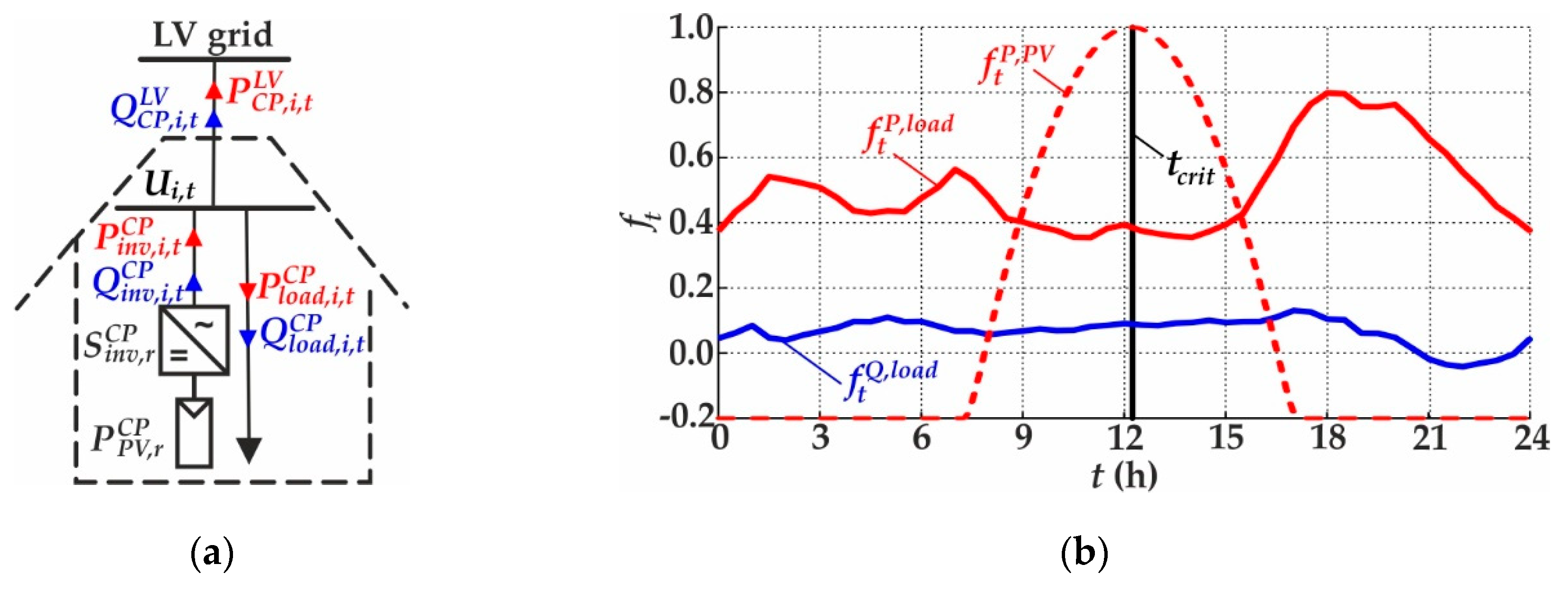
Figure 2a shows the used customer plant structure. It has two components: the load or power consumption and the electricity production. For each customer plant i and time-point t, it is characterized by the active and reactive power consumption and production of the internal loads ($P_{load,i,t}^{CP}$ and $Q_{load,i,t}^{CP}$) and the PV-system ( $P_{inv,i,t}^{CP}$ and $Q_{inv,i,t}^{CP}$), respectively. The active $P_{CP,i,t}^{LV}$ and reactive power $Q_{CP,i,t}^{LV}$ flows from the CP i to LV_link-grid at time-point t are given by:

$$P_{CP,i,t}^{LV}=P_{inv,i,t}^{CP}-P_{load,i,t}^{CP},$$

(2a)

$$Q_{CP,i,t}^{LV}=Q_{inv,i,t}^{CP}-Q_{load,i,t}^{CP}$$

(2b)

Each CP is connected to a boundary link node (BLiN) of the corresponding LV_link-grid with the actual $U_{i,t}$ and nominal voltage $U_{nom}^{LV}$, and includes a PV-system with a module-rating of $P_{PV,r}^{CP}=5$ kW [24] and an inverter-rating of $S_{inv,r}^{CP}=P_{PV,r}^{CP}/0.9$ [25].

Figure 2b shows the load and production profiles represented by solid and dashed lines, respectively. Active and reactive power are coloured red and blue, respectively. The critical time-point $t_{\mathit{crit}}$, where the maximal PV production occurs, is marked as a black vertical line. The profiles determine the active and reactive power consumption of loads for nominal grid voltage ($P_{nom,t}^{load}$ and $Q_{nom,t}^{load}$) and the active power production of the PV-system, as in:

$$P_{nom,t}^{load}=f_t^{P,load}·P_{peak}^{load},$$

(3a)

$$Q_{nom,t}^{load}=f_t^{Q,load}·P_{peak}^{load}$$

(3b)

$$P_{inv,i,t}^{CP}=f_t^{P,PV}·P_{PV,r}^{CP}$$

(3c)

where $f_t^{P,load}$ and $f_t^{Q,load}$ are the active and reactive power load profile factors at time-point t; $f_t^{P,PV}$ is the active power production profile factor at time-point t; and $P_{peak}^{load}=1.368$ kW is the peak active power demand (the value of $P_{peak}^{load}$ is calculated based on the maximum 15-minutes mean value of the active power flow measured throughout 2016 at the secondary side of the DTR of the real LV_link-grid described in Section 2.2.2 [24]) of each CP’s load. The reactive power contribution of PV-systems is determined by the applied control strategy as described in Section 2.3. It is interesting to note that nowadays the load has changed the behaviour in terms of reactive power. The load behaves capacitive in the evening because the residential customers have mainly turned to LED lighting [26].

The load voltage dependency is modelled with a ZIP model according to:

$$P_{load,i,t}^{CP}=P_{nom,t}^{load}·\left(C_t^{P,Z}·{\left(U_{i,t}/U_{nom}^{LV}\right)}^2+C_t^{P,I}·\left(U_{i,t}/U_{nom}^{LV}\right)+C_t^{P,P}\right)$$

(4a)

$$Q_{load,i,t}^{CP}=Q_{nom,t}^{load}·\left(C_t^{Q,Z}·{\left(U_{i,t}/U_{nom}^{LV}\right)}^2+C_t^{Q,I}·\left(U_{i,t}/U_{nom}^{LV}\right)+C_t^{Q,P}\right)$$

(4b)

where $C_t^{P,Z}$, $C_t^{P,I}$, $C_t^{P,P}$ and $C_t^{Q,Z}$, $C_t^{Q,I}$, $C_t^{Q,P}$ are the active and reactive power ZIP coefficients at time-point t. ZIP coefficients and load profiles are given for the considered 24 h time horizon in [26,27]. The load and production profiles shown in Figure 2b are sampled into $\Delta t=15\min$ time-steps, resulting in $N=24\mathrm{h}/\Delta t=96$ load-flow simulations per scenario.

2.2.2. Distribution Grid Models

MV and LV levels are modelled and simulated in a common model. For the sake of simplicity, they are described separately below.

(A) Low Voltage Grid

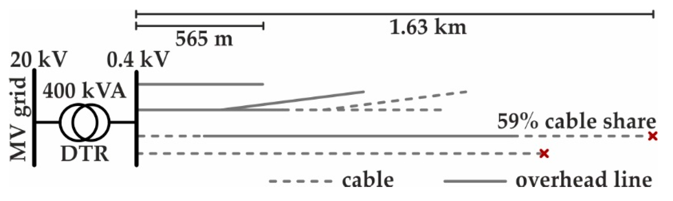
Figure 3 shows a simplified one-line diagram of the used LV_link-grid model.

It is a real rural grid with four feeders with a minimum and maximum length of 565 m and 1.63 km, respectively. In this link-grid with a cable share of about 59% and a nominal voltage of $U_{nom}^{LV}=0.4\mathrm{kV}$ are connected 61 residential customers. It is connected to the MV_link-grid through a 21 kV/0.42 kV, 400 kVA DTR with its tap changer fixed in mid-position. The detailed LV_link-grid model data (instead of the 160 kVA DTR given in the mentioned reference, a 400 kVA one with a rated primary and secondary voltage of 21 kV and 0.42 kV, respectively, and a short circuit voltage of 3.7% with a resistive part of 1% is used, because of the high PV share. The tap changer is fixed in its mid-position) is given in [28]. Figure 3 shows with red crosses the connection points of the L(U)s.

(B) Medium Voltage Grid

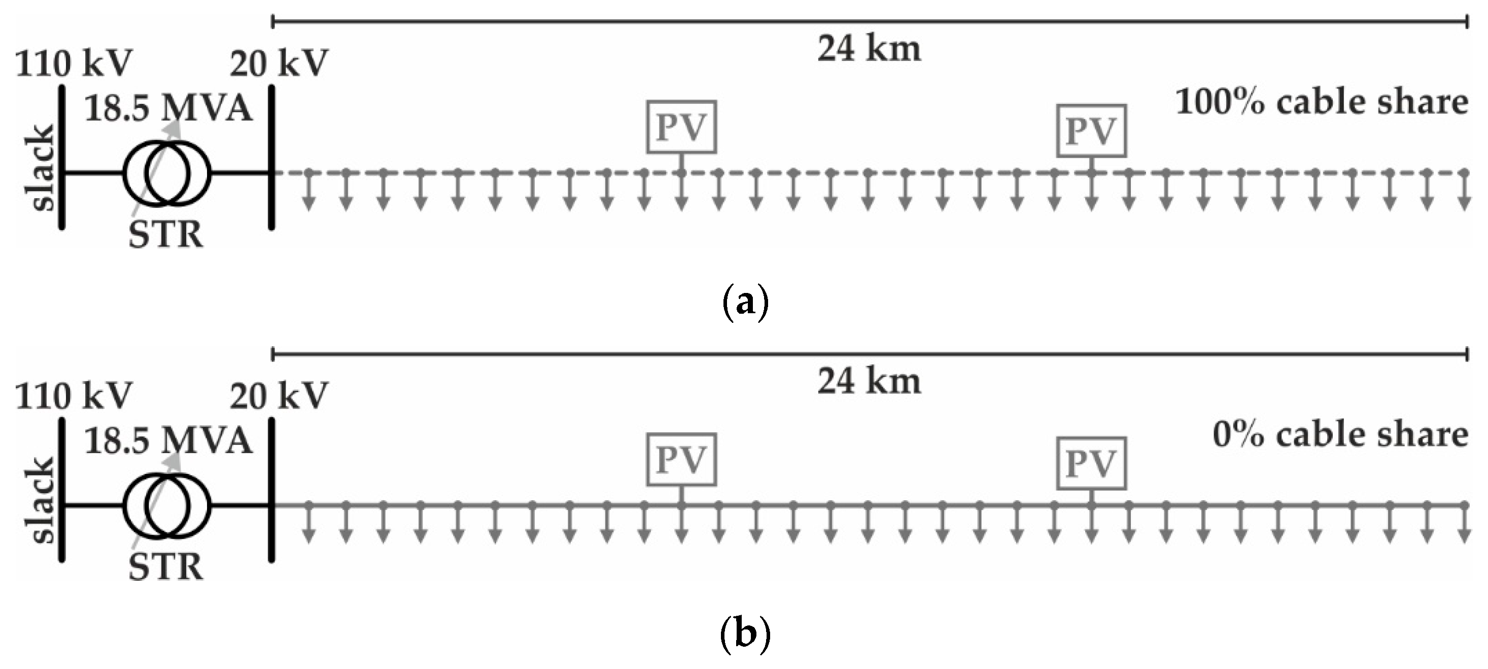
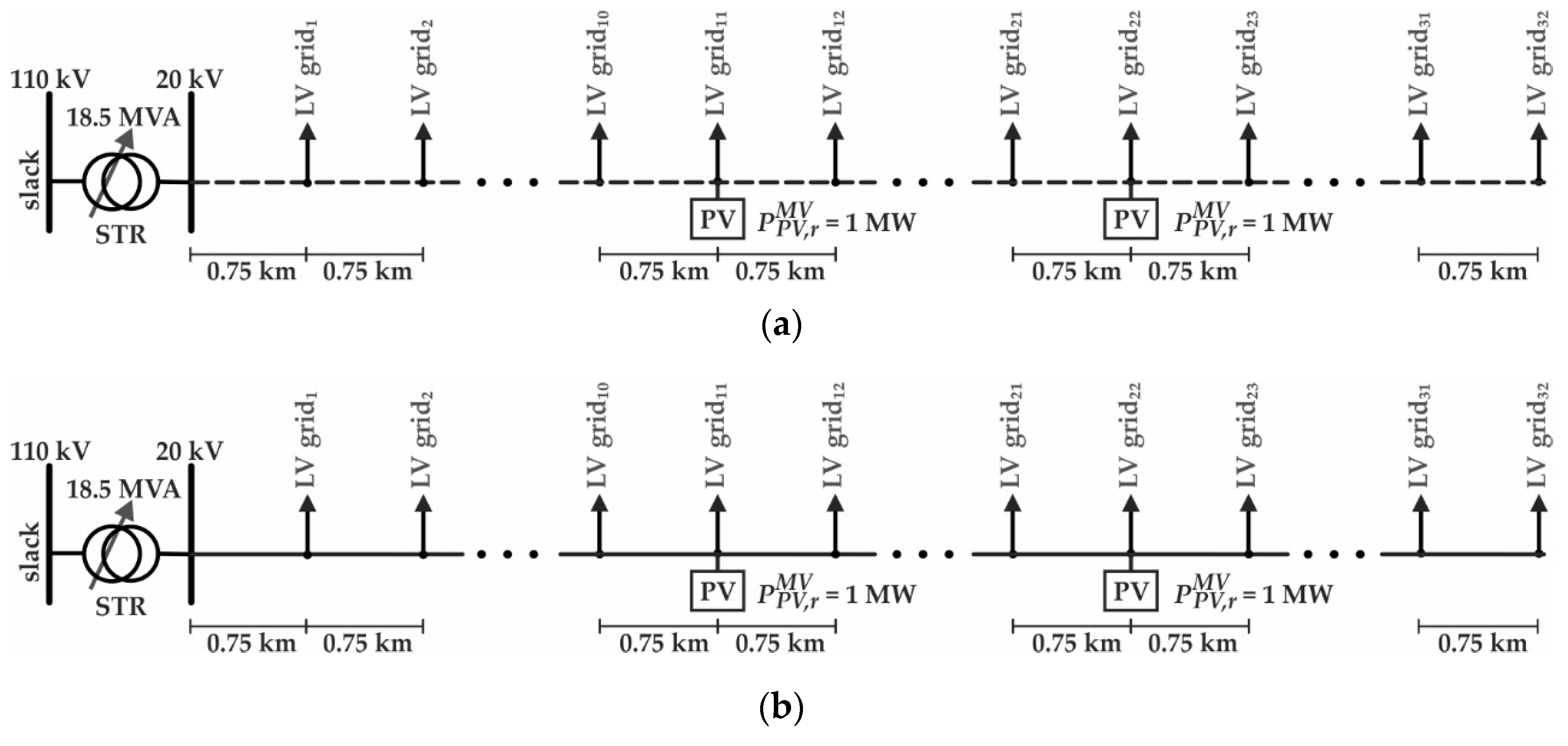
Figure 4 shows a simplified one-line diagrams of the used MV_link-grids. Both MV_link-grids are identical, except for the conductor type: Figure 4a,b represent the cases with cable and overhead conductors in MV level, respectively. To each MV_link-grid are connected 32 LV_link-grids and two PV-systems, each with a module and inverter rating of $P_{\mathit{PV},r}^{\mathrm{MV}}=1$ MW and $S_{\mathit{inv},r}^{\mathit{MV}}=1$ MVA, respectively. The active power production $P_{inv,t}^{MV}$ of each PV-system connected to the MV_link-grid at time-point t is determined by:

$$P_{inv,t}^{MV}=f_t^{P,PV}·P_{PV,r}^{MV}$$

(5)

while the reactive power contribution is determined by the applied control strategy as described in Section 2.3. The MV feeder length is 24 km and slack voltage is set to the nominal value of 110 kV. The detailed data of the MV_link-grid models is given in Appendix A.

2.3. Simulated Control Setups

The use of the reactive power to control the voltage in LV grids leads to an uncontrolled reactive power flow up to the HV grid, reducing its RPM. This uncontrolled reactive power flow can be practically compensated by CDs connected at different points of the grid. Therefore, a series of simulations is performed to investigate the grid behaviour for various placements of CDs when the VVC chain strategy is used. The grid-link setups are set assuming that the same DSO owns and operates the MV and LV grids. They are derived from the generalized VVC chain strategy shown in Figure 1. The five identified cases are depicted in Figure 5, Figure 6, Figure 7, Figure 8 and Figure 9. For each case is derived a specific equation from the generalized form presented in Equation (1) that describes all elements involved in the VVC chain, Equations (6)–(10). It is supposed that neither DSts nor DGs are connected to the LV_link-grids. One of the basic principles in setting up the grid-links is the minimization of the number of secondary and primary control units to keep the CapEx and OpEx as low as possible. Therefore, no VVSC is provided for the LV_grid-link, since only L(U) local controls (${\mathrm{var}\mathbf{LC}}_{\mathrm{L}\left(\mathrm{U}\right)}^{\mathrm{LV}})$ are connected at the end of some laterals: coordination is not relevant. The LV_grid-link is shown in gold-coloured dotted lines because its existence must be discussed also in terms of load-generation balancing. The latter is not within the scope of this paper. A grid-link is set up in the MV level. Here, the VVSC is important to coordinate the Q-contribution of DGs, RDs and the neighbour grid-links with the voltage at the secondary side or OLTC position of the supplying transformer (STR) while respecting all constraints and optimizing the network performance at the same time.

All simulations are performed using both distribution grid models. The STR tap is fixed in its mid-position so that the impact of CD placement on distribution grid behaviour can be clearly analysed.

1. Control setup: Without any var control (no control)

Figure 5 shows the simplified form of the VVC chain strategy representing the setup without any var control. In this form, the VVC chain in the Y-axis is presented by the following generalized equation:

$${\mathrm{VVC}}^{\mathrm{Y}-\mathrm{axis}}{=\{\mathrm{VV}\mathbf{SC}}^{\mathrm{MV}}\left({\mathrm{var}\mathbf{PC}}_{\mathrm{DG}}^{\mathrm{MV}}\right)\}$$

(6)

Usually, ${\mathrm{VV}\mathbf{SC}}^{\mathrm{MV}}$ sends the var set-points ${\mathrm{Q}}_{\mathit{DG}}^{\mathit{MV}*}$ to all DGs connected to the MV_link-grid. In our simulations, all DGs, i.e., PV-systems, inject into the grid with a power factor of one, ${\mathrm{Q}}_{\mathit{DG}}^{\mathit{MV}*}=0$. PV-systems in CP level inject with a power factor of one as well. Therefore, the LV grids supply reactive power to the loads connected at the CP level.

In this control setup, reactive power is exchanged between all three levels: between HV_ and MV_link-grid, MV_ and LV_link-grids, and LV_link-grids and CPs.

2. Control setup: L(U)-control and CP_Q-autarky (no CDs)

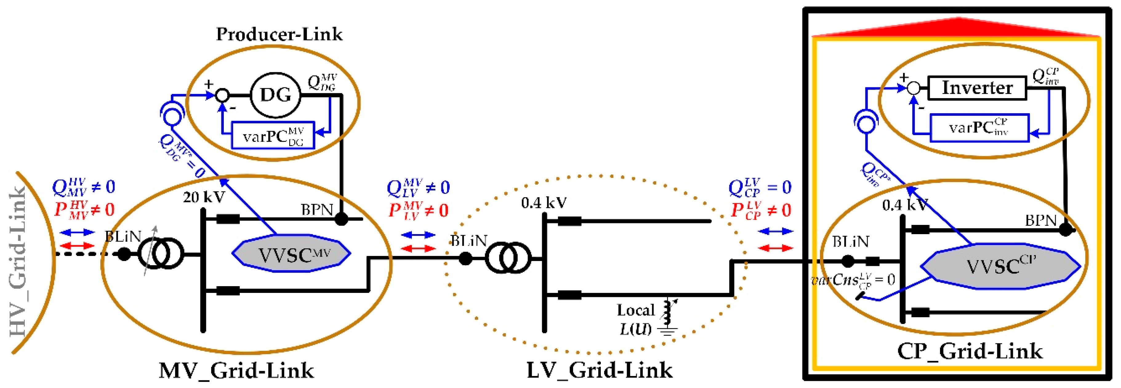
Figure 6 depicts the simplified form of the VVC chain strategy representing the setup with L(U)-control and CP_Q-autarky. In this form, the VVC chain in the Y-axis is presented by the following equation:

$${\mathrm{VVC}}^{Y-\mathrm{axis}}{=\{\mathrm{VVSC}}^{\mathrm{MV}}\left({\mathrm{var}\mathbf{PC}}_{\mathrm{DG}}^{\mathrm{MV}}\right){,\mathrm{var}\mathbf{LC}}_{\mathrm{L}\left(\mathrm{U}\right)}^{\mathrm{LV}}{,\mathrm{VV}\mathbf{SC}}^{\mathrm{CP}}\left({\mathrm{var}\mathbf{PC}}_{\mathrm{inv}}^{\mathrm{CP}}{,\mathrm{var}\mathbf{Cns}}_{\mathrm{CP}}^{\mathrm{LV}}=0\right)\}$$

(7)

The ${\mathrm{VV}\mathbf{SC}}^{\mathrm{MV}}$ sends the var set-points ${\mathrm{Q}}_{\mathit{DG}}^{\mathit{MV}*}=0$ to all PV-systems connected to the MV_link-grid. To alleviate upper voltage limit violations, ${\mathrm{var}\mathbf{LC}}_{\mathrm{L}\left(\mathrm{U}\right)}^{\mathrm{LV}}$ are set at the ends of the violated LV feeders (see Figure 3). Each ${\mathrm{VV}\mathbf{SC}}^{\mathrm{CP}}$ sends the required var set-point ${\mathrm{Q}}_{\mathit{inv}}^{\mathit{CP}*}$ to the corresponding PV-system to achieve Q-autarky, i.e., full reactive power compensation in CP level, satisfying the var constraint ${\mathrm{var}\mathbf{Cns}}_{\mathrm{CP}}^{\mathrm{LV}}=0$ at all times [18].

In this control setup, reactive power is exchanged between two levels: between HV_ and MV_link-grid and between MV_ and LV_link-grids.

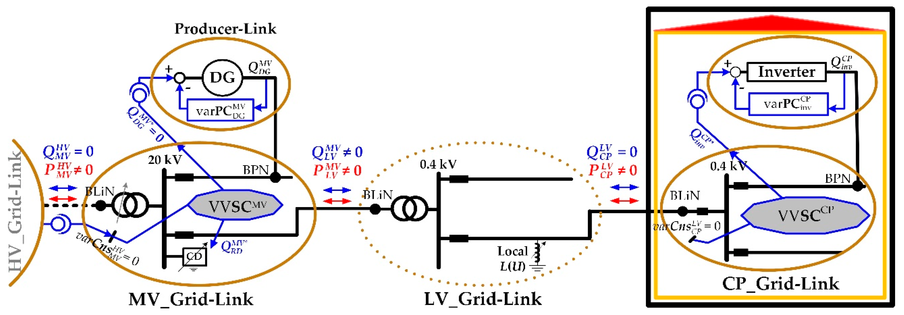
3. Control setup: L(U)-control, CP_Q-Autarky and CD at the STR MV-busbar (${\mathit{CD}}_{\mathit{MV}}^{\mathit{STR}}$)

This control setup is derived from the second one and supplemented with a CD connected to the STR MV-bus bar, Figure 7. The VVC chain in the Y-axis is presented as follows:

$${\mathrm{VVC}}^{\mathrm{Y}-\mathrm{axis}}{=\{\mathrm{VV}\mathbf{SC}}^{\mathrm{MV}}\left({\mathrm{var}\mathbf{PC}}_{\mathrm{CD}}^{\mathrm{MV}}{,\mathrm{var}\mathbf{PC}}_{\mathrm{DG}}^{\mathrm{MV}}{,\mathrm{var}\mathbf{Cns}}_{\mathrm{MV}}^{\mathrm{HV}}=0\right){,\mathrm{var}\mathbf{LC}}_{\mathrm{L}\left(\mathrm{U}\right)}^{\mathrm{LV}}{,\mathrm{VV}\mathbf{SC}}^{\mathrm{CP}}\left({\mathrm{var}\mathbf{PC}}_{\mathrm{inv}}^{\mathrm{CP}}{,\mathrm{var}\mathbf{Cns}}_{\mathrm{CP}}^{\mathrm{LV}}=0\right)\}$$

(8)

For the simulations, the CD is parametrized to respect the constraint ${\mathrm{var}\mathbf{Cns}}_{\mathrm{MV}}^{\mathrm{HV}}=0$. Therefore, the reactive power is exchanged only between MV_ and LV_link-grids.

4. Control setup: L(U)-control, CP_Q-Autarky and CD at the DTRs’ MV-busbars (${\mathit{CD}}_{\mathit{MV}}^{\mathit{DTR}}$)

In this case, CD positioning is moved from the MV-bus bar of the STR to the MV-bus bars of the DTRs, compensating the reactive power required by LV_link-grids, Figure 8. The VVC chain in the Y-axis is presented by the following equation:

$${\mathrm{VVC}}^{\mathrm{Y}-\mathrm{axis}}{=\{\mathrm{VV}\mathbf{SC}}^{\mathrm{MV}}\left({\mathrm{var}\mathbf{PC}}_{\mathrm{DG}}^{\mathrm{MV}},{\mathrm{var}\mathbf{PC}}_{\mathrm{CD}}^{\mathrm{MV}},{\mathrm{var}\mathbf{Cns}}_{\mathrm{LV}}^{\mathrm{MV}}=0\right){,\mathrm{var}\mathbf{LC}}_{\mathrm{L}\left(\mathrm{U}\right)}^{\mathrm{LV}}{,\mathrm{VV}\mathbf{SC}}^{\mathrm{CP}}\left({\mathrm{var}\mathbf{PC}}_{\mathrm{inv}}^{\mathrm{CP}}{,\mathrm{var}\mathbf{Cns}}_{\mathrm{CP}}^{\mathrm{LV}}=0\right)\}$$

(9)

Therefore, the reactive power is exchanged only between HV_ and MV_link-grid.

5. Control setup: L(U)-control, CP_Q-Autarky and CDs at the DTRs’ LV-busbars (${\mathit{CD}}_{\mathit{LV}}^{\mathit{DTR}}$)

Here, CD positioning is moved from the MV- to the LV-bus bars of DTRs, compensating the reactive power required by LV_link-grid, Figure 9. The VVC chain in the Y-axis is presented by:

$${\mathrm{VVC}}^{\mathrm{Y}-\mathrm{axis}}{=\{\mathrm{VV}\mathbf{SC}}^{\mathrm{MV}}\left({\mathrm{var}\mathbf{PC}}_{\mathrm{DG}}^{\mathrm{MV}},{\mathrm{var}\mathbf{PC}}_{\mathrm{CD}}^{\mathrm{LV}},{\mathrm{var}\mathbf{Cns}}_{\mathrm{LV}}^{\mathrm{MV}}=0\right){,\mathrm{var}\mathbf{PC}}_{\mathrm{L}\left(\mathrm{U}\right)}^{\mathrm{LV}}{,\mathrm{VV}\mathbf{SC}}^{\mathrm{CP}}\left({\mathrm{var}\mathbf{PC}}_{\mathrm{inv}}^{\mathrm{CP}}{,\mathrm{var}\mathbf{Cns}}_{\mathrm{CP}}^{\mathrm{LV}}=0\right)\}$$

(10)

Also in this case, the reactive power is exchanged only between HV_ and MV_link-grid.

3. Results and Discussion

The behaviour of both distribution grids is described below for the simulated control setups; thereby, the effect of CD placement is analysed in detail. Based on these results, the optimal setup of the volt/var control chain is discussed.

3.1. Behaviour of Distribution Grids

As explained in Section 2.2.2, all simulations are performed in the common model of MV and LV levels. Simulation results over the 24 h time horizon are shown graphically in Figures 10 and 12 for the cable and overhead line structure, respectively. Whereas in

Table 2. Behaviour of the distribution grid with cable conductors in MV level at $t_{\mathit{crit}}$ for different control setups.

Control Setup	${\mathit{Q}}_{\mathit{t}\mathit{o}\mathit{t},{\mathit{t}}_{\mathit{c}\mathit{r}\mathit{i}\mathit{t}}}^{\mathit{L}\left(\mathit{U}\right)}$ (Mvar)	${\mathit{Q}}_{\mathit{t}\mathit{o}\mathit{t},{\mathit{t}}_{\mathit{c}\mathit{r}\mathit{i}\mathit{t}}}^{\mathit{C}\mathit{D}}$ (Mvar)	${\mathit{Q}}_{\mathit{M}\mathit{V},{\mathit{t}}_{\mathit{c}\mathit{r}\mathit{i}\mathit{t}}}^{\mathit{H}\mathit{V}}$ (Mvar)	${\mathit{P}}_{{\mathit{t}}_{\mathit{c}\mathit{r}\mathit{i}\mathit{t}}}^{\mathit{l}\mathit{o}\mathit{s}\mathit{s}}$ (MW)	$\mathit{L}\mathit{o}\mathit{a}\mathit{d}\mathit{i}\mathit{n}{\mathit{g}}_{{\mathit{t}}_{\mathit{c}\mathit{r}\mathit{i}\mathit{t}}}^{\mathit{S}\mathit{T}\mathit{R}}$ (%)	$\mathit{L}\mathit{o}\mathit{a}\mathit{d}\mathit{i}\mathit{n}{\mathit{g}}_{{\mathit{t}}_{\mathit{c}\mathit{r}\mathit{i}\mathit{t}}}^{\overline{\mathit{D}\mathit{T}\mathit{R}\mathit{s}}}$ (%)
No control	0.00	0.00	−0.70	0.94	52.44	64.40
No CDs	2.07	0.00	−2.65	1.17	53.28	67.47
${\mathbf{CD}}_{\mathbf{MV}}^{\mathbf{STR}}$	2.63	−3.17	0.00	1.23	50.95	67.74
${\mathbf{CD}}_{\mathbf{MV}}^{\mathbf{DTR}}$	3.03	−3.67	0.11	1.25	50.81	68.11
${\mathbf{CD}}_{\mathbf{LV}}^{\mathbf{DTR}}$	3.60	−4.24	0.11	1.33	50.35	60.74

and

Table 3. Behaviour of the distribution grid with overhead conductors in MV level at $t_{\mathit{crit}}$ for different control setups.

Control Setup	${\mathit{Q}}_{\mathit{t}\mathit{o}\mathit{t},{\mathit{t}}_{\mathit{c}\mathit{r}\mathit{i}\mathit{t}}}^{\mathbf{L}\left(\mathbf{U}\right)}$ (Mvar)	${\mathit{Q}}_{\mathit{t}\mathit{o}\mathit{t},{\mathit{t}}_{\mathit{c}\mathit{r}\mathit{i}\mathit{t}}}^{\mathit{C}\mathit{D}}$ (Mvar)	${\mathit{Q}}_{\mathit{M}\mathit{V},{\mathit{t}}_{\mathit{c}\mathit{r}\mathit{i}\mathit{t}}}^{\mathit{H}\mathit{V}}$ (Mvar)	${\mathit{P}}_{{\mathit{t}}_{\mathit{c}\mathit{r}\mathit{i}\mathit{t}}}^{\mathit{l}\mathit{o}\mathit{s}\mathit{s}}$ (MW)	$\mathit{L}\mathit{o}\mathit{a}\mathit{d}\mathit{i}\mathit{n}{\mathit{g}}_{{\mathit{t}}_{\mathit{c}\mathit{r}\mathit{i}\mathit{t}}}^{\mathit{S}\mathit{T}\mathit{R}}$ (%)	$\mathit{L}\mathit{o}\mathit{a}\mathit{d}\mathit{i}\mathit{n}{\mathit{g}}_{{\mathit{t}}_{\mathit{c}\mathit{r}\mathit{i}\mathit{t}}}^{\overline{\mathit{D}\mathit{T}\mathit{R}\mathit{s}}}$ (%)
No control	0.00	0.00	−1.97	1.22	51.85	63.53
No CDs	2.11	0.00	−4.04	1.52	54.03	67.61
${\mathbf{CD}}_{\mathbf{MV}}^{\mathbf{STR}}$	2.79	−4.66	0.00	1.60	48.93	67.90
${\mathbf{CD}}_{\mathbf{MV}}^{\mathbf{DTR}}$	3.80	−4.52	−1.08	1.63	49.04	69.42
${\mathbf{CD}}_{\mathbf{LV}}^{\mathbf{DTR}}$	4.40	−5.11	−1.06	1.72	48.50	58.49

results at t_crit are listed. Simulations are made for different control setups; results are drown in different colours as follows: “no control“ in dashed blackline; “no CDs” in purple; “${\mathrm{CD}}_{\mathrm{MV}}^{\mathrm{STR}}$” in green; “${\mathrm{CD}}_{\mathrm{MV}}^{\mathrm{DTR}}$” in ocra yellow and “${\mathrm{CD}}_{\mathrm{LV}}^{\mathrm{DTR}}$” in red solid line. The behaviour of distribution grids is analysed using various parameters as:

(a)

the total reactive power consumption of all L(U)s included in the LV_link-grids, $Q_{\mathit{tot}\mathbf{,}\mathit{t}}^{\mathit{L}\mathbf{\left(}\mathit{U}\mathbf{\right)}}$;

(b)

the total reactive power contribution of all CDs included in MV_ or LV_link-grids, ${\mathit{Q}}_{\mathit{tot}\mathbf{,}\mathit{t}}^{\mathit{CD}}$;

(c)

the reactive power exchange between HV_ and MV_link-grid, ${\mathit{Q}}_{\mathit{MV},\mathit{t}}^{\mathit{HV}}$, at the STR primary side;

(d)

the active power losses of the distribution grid, ${\mathit{P}}_{\mathit{t}}^{\mathit{loss}}$, including losses of transformers, cables and overhead lines;

(e)

the STR loading, ${\mathit{Loading}}_t^{\mathit{STR}}$;

(f)

the mean loading of all DTRs, ${\mathit{Loading}}_t^{\overline{\mathit{DTRs}}}$, which is calculated as in

$${\mathit{Loading}}_t^{\overline{\mathit{DTRs}}}=\frac{{\sum }_{\mathrm{k}=1}^{32}{\mathit{Loading}}_{k,t}^{\mathit{DTR}}}{32}$$

(11)

where ${\mathit{Loading}}_{k,t}^{\mathit{DTR}}$ is the loading of the DTR k at time-point t, and 32 is the number of DTRs;

(g)

the voltage limit violation index, ${\mathit{VI}}_{\mathit{t}}$, which is calculated as in

$${\mathit{VI}}_t=\frac{{\sum }_{j=1}^{m_t}\left(U_{u,t}^{\mathit{upper}}{-U}_{\mathit{lim}}^{\mathit{upper}}\right)}{U_{\mathit{nom}}^{\mathit{LV}}}+\frac{{\sum }_{j=1}^{n_t}\left(U_{\mathit{lim}}^{\mathit{lower}}{-U}_{v,t}^{\mathit{lower}}\right)}{U_{\mathit{nom}}^{\mathit{LV}}}$$

(12)

where $m_t$ is the number of LV_link-grid nodes that violate the upper voltage limit at time-point t; $n_t$ is the number of LV_link-grid nodes that violate the lower voltage limit at time-point t; $U_{u,t}^{\mathit{upper}}$ is the voltage of the LV_link-grid node u with upper voltage limit violation at time-point t; $U_{v,t}^{\mathit{lower}}$ is the voltage of the LV_link-grid node v with lower voltage limit violation at time-point t; $U_{\mathit{lim}}^{\mathit{upper}}=1.1·U_{\mathit{nom}}^{\mathit{LV}}=0.44\mathrm{kV}$ is the upper voltage limit; and $U_{\mathit{lim}}^{\mathit{lower}}=0.9·U_{\mathit{nom}}^{\mathit{LV}}=0.36\mathrm{kV}$ is the lower voltage limit. Only LV_link-grid nodes are considered because the simulations show that no voltage limit violations appear in the MV_link-grid.

Simulations show that the currents through the transformers, cables and overhead lines never exceed their thermal ratings. The behaviour of distribution grids strongly depends on the PV injections and the placement of CDs.

3.1.1. Distribution Grid with Cable Conductors in MV Level

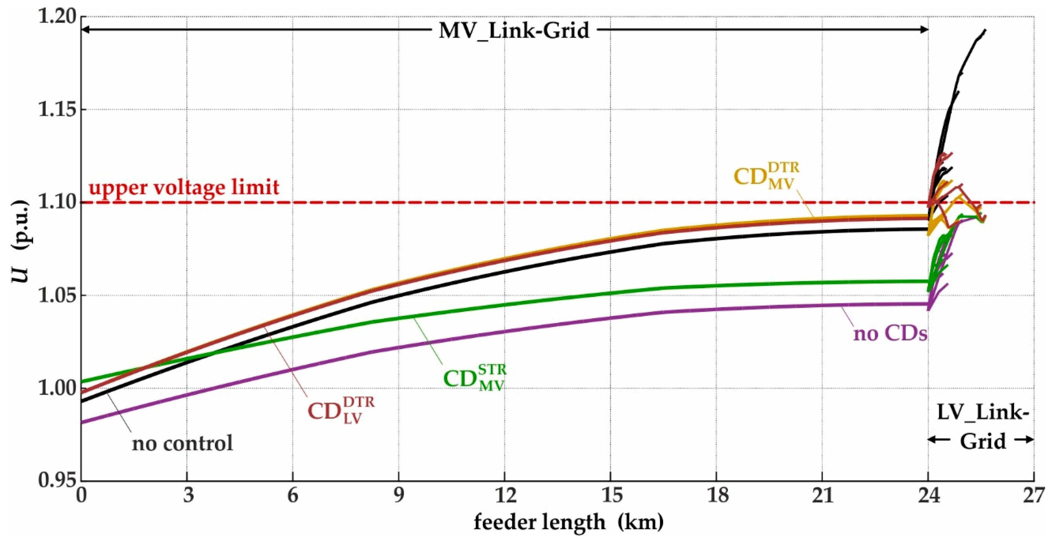
Figure 10 shows the voltage profiles of the MV_link-grid with cable conductors and the backmost LV_link-grid for the critical time-point $t_{\mathit{crit}}$.

Without any var control, the upper voltage limit is violated with a voltage limit violation index of 35.51. In the case of “no CDs”, “${\mathrm{CD}}_{\mathrm{MV}}^{\mathrm{STR}}$” and “${\mathrm{CD}}_{\mathrm{MV}}^{\mathrm{DTR}}$”, no voltage limit violations appear, but if CDs are installed at the DTRs’ LV-busbars, the upper voltage limit is violated with a voltage limit violation index of 0.04.

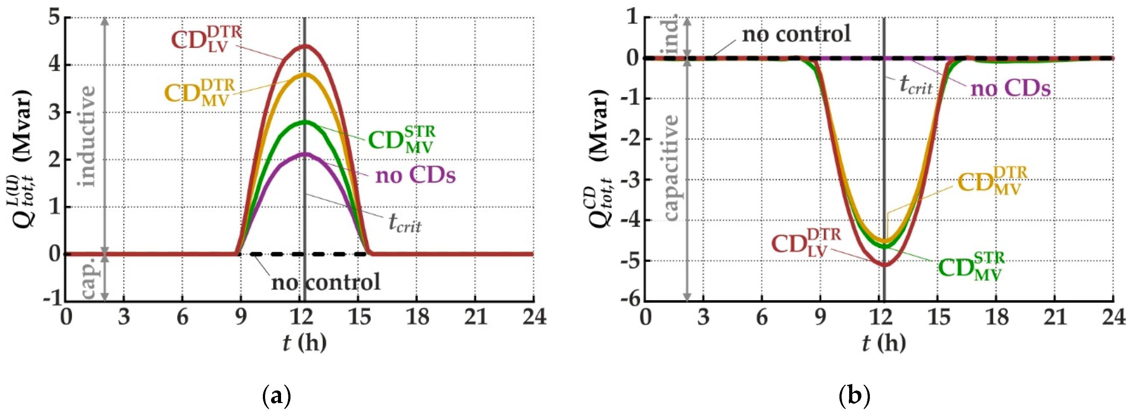
Figure 11 shows the behaviour of the distribution grid with cable conductors in MV level over the 24 h time horizon for all control setups. Figure 11a shows the total reactive power consumption of all L(U)s connected at the distribution grid. When “no control” is applied, no L(U)s are installed and as a result, there is no Q-consumption. The maximum total Q-consumption of L(U)s is reached at t_crit for all cases. The lowest value of 2.07 Mvar is achieved when no CDs are applied, while the highest one of 3.60 Mvar is reached when CDs are installed at the secondary sides of DTRs.

Figure 11b shows the reactive power contribution of the CDs. In the cases of “no control” and “no CDs”, no CDs are installed, thus no Q-contribution is expected. In the other cases, the maximum Q-contribution of CDs appears at $t_{\mathit{crit}}$. The ${\mathrm{CD}}_{\mathrm{MV}}^{\mathrm{STR}}$ behaves inductive in time periods 0:00 to 9:20 a.m. and 03:00 to 12:00 p.m. to compensate the capacitive power produced by the cable. As the PV injection increases from 9:00 a.m., the L(U)s included in LV_link-grid begin to consume inductive power to eliminate the upper voltage limit violations. To compensate the additionally required inductive power, the reactive power production of ${\mathrm{CD}}_{\mathrm{MV}}^{\mathrm{STR}}$ changes from inductive to capacitive, reaching the maximum Q-injection of 3.17 Mvar. When CDs are installed in distribution substation, they behave purely capacitive with a maximum Q-injection of 3.67 and 4.24 Mvar for the cases “${\mathrm{CD}}_{\mathrm{MV}}^{\mathrm{DTR}}$” and “${\mathrm{CD}}_{\mathrm{LV}}^{\mathrm{DTR}}$”, respectively.

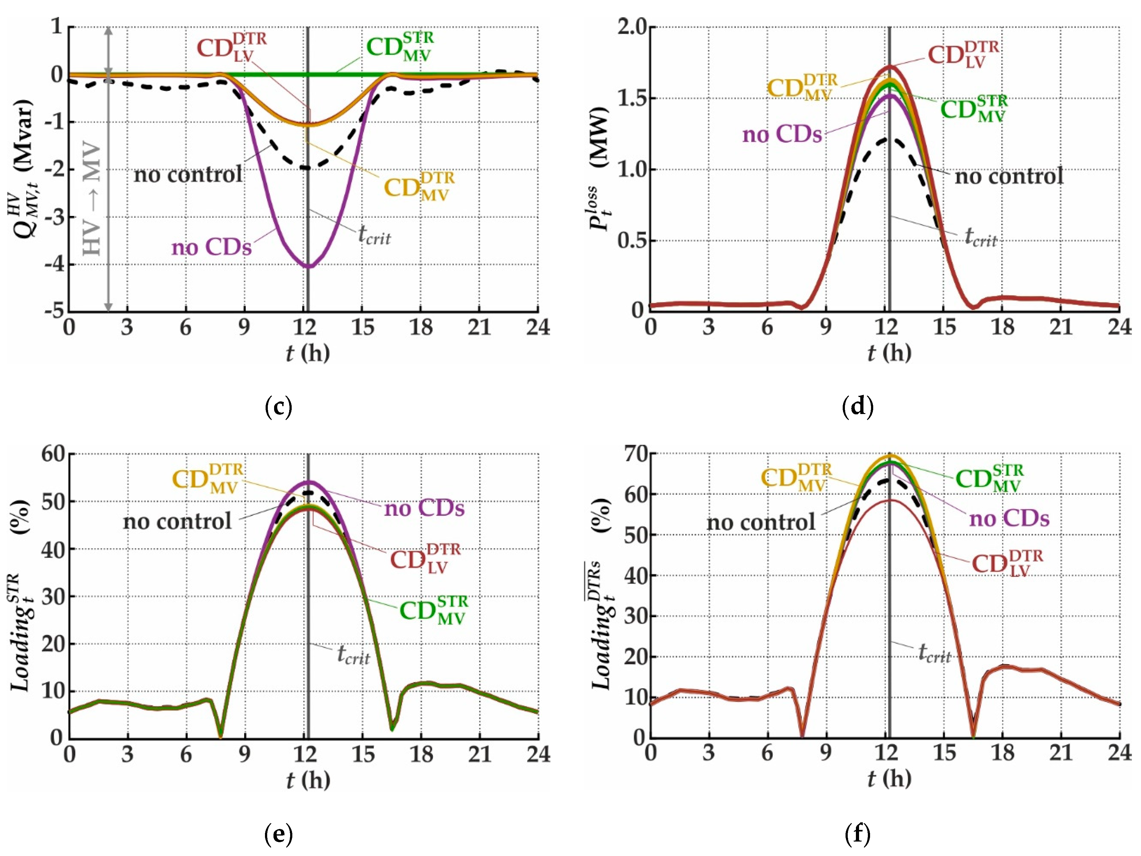
Figure 11c shows the reactive power exchange between HV_ and MV_link-grid. In the control setups “no control” and “no CDs”, the MV_link-grid draws reactive power from the HV_link-grid between approx. 9:30 a.m. and 3:00 p.m. In the remaining time horizon, the MV_link-grid injects reactive power into the HV_link-grid. In the case “no control”, two peaks of $Q_{MV,t}^{HV}$ are identified: one at $t_{\mathit{crit}},$ where the MV_link-grid draws 0.70 Mvar from the HV_link-grid; and the other at 10 p.m., where the MV_link-grid injects 0.80 Mvar into the HV_link-grid. This behaviour is caused by the capacitive nature of the load in the evening and the cable structure of the MV_link-grid. In the case of “no CDs”, the MV_link-grid draws the maximum reactive power of 2.65 Mvar from the HV_link-grid at $t_{\mathit{crit}}.$ If the CD is installed at the STR MV-busbar, no reactive power is exchanged between HV_ and MV_link-grid over the all-time horizon. In the control setups “${\mathrm{CD}}_{\mathrm{MV}}^{\mathrm{DTR}}$” and “${\mathrm{CD}}_{\mathrm{LV}}^{\mathrm{DTR}}$”, the MV_link-grid injects reactive power into HV_link-grid over the all-time horizon, showing their minimum Q-injection of 0.11 Mvar at $t_{\mathit{crit}}$.

Figure 11d shows the active power losses of the distribution grid. In all cases, losses increase drastically between approx. 8:00 a.m. and 4:30 p.m. due to the PV injection. The maximum values appear at $t_{\mathit{crit}}$, where the control setup “${\mathrm{CD}}_{\mathrm{LV}}^{\mathrm{DTR}}$” provokes the highest grid losses of 1.33 MW.

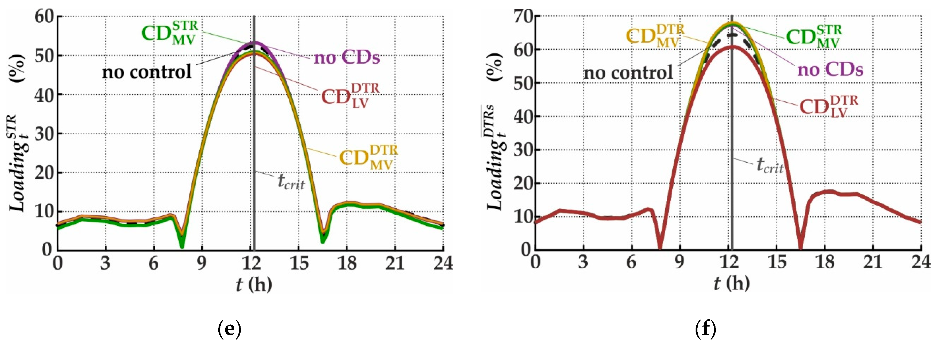
Figure 11e,f show the STR and mean DTR loading, respectively. In all cases, STR and mean DTR loading increase drastically between approx. 8:00 a.m. and 4:30 p.m. due to PV injections, reaching their maximum values at $t_{\mathit{crit}}$. For the STR loading, the highest value of 53.28% is reached for the control setup “no CDs”; while the lowest one of 50.35% is reached for the “${\mathrm{CD}}_{\mathrm{LV}}^{\mathrm{DTR}}$” case. For the mean DTR loading, the highest value of 68.11% is reached for the control setup “${\mathrm{CD}}_{\mathrm{MV}}^{\mathrm{DTR}}$”; while the lowest one of 60.74% is reached for the “${\mathrm{CD}}_{\mathrm{LV}}^{\mathrm{DTR}}$” case.

3.1.2. Distribution Grid with Overhead Conductors in MV Level

Figure 12 shows the voltage profiles of the MV_link-grid with overhead line conductors and the backmost LV_link-grid for the critical time-point $t_{\mathit{crit}}.$

Without any var control, the upper voltage limit is violated with a voltage limit violation index of 58.38. In the case of “no CDs” and “${\mathrm{CD}}_{\mathrm{MV}}^{\mathrm{STR}}$”, no voltage limit violations appear, but if CDs are installed at distribution substation, the upper voltage limit is violated with a voltage limit violation index of 1.79 and 7.73, respectively, for the cases “${\mathrm{CD}}_{\mathrm{MV}}^{\mathrm{DTR}}$” and “${\mathrm{CD}}_{\mathrm{LV}}^{\mathrm{DTR}}$”.

Figure 13 shows the behaviour of the distribution grid with overhead line conductors in MV level over the 24 h time horizon for all control setups. Figure 13a shows the total reactive power consumption of all L(U)s connected at the distribution grid. When “no control” is applied, no L(U)s are installed and as a result, there is no Q-consumption. The maximum total Q-consumption of L(U)s is reached at t_crit for all cases. The lowest value of 2.11 Mvar is achieved when no CDs are applied, while the highest one of 4.40 Mvar is reached when CDs are installed at the secondary sides of DTRs.

Figure 13b shows the reactive power contribution of the CDs. In the cases of “no control” and “no CDs”, no CDs are installed, thus no Q-contribution is expected. If CDs are installed, they behave purely capacitive, reaching their maximum Q-contribution at $t_{\mathit{crit}}$. The lowest value of 4.52 Mvar is achieved when CDs are installed at the DTRs’ primary sides, while the highest one of 5.11 Mvar is reached when they are installed at the DTRs’ secondary sides.

Figure 13c shows the reactive power exchange between HV_ and MV_link-grid. In the control setup “no control”, the MV_link-grid injects reactive power into the HV_link-grid between approx. 9:00 p.m. and 11:15 p.m. In the remaining time horizon, the MV_link-grid draws reactive power from the HV_link-grid; two peaks of $Q_{MV,t}^{HV}$ are identified: one at $t_{\mathit{crit}}$, where the MV_link-grid draws 1.97 Mvar from the HV_link-grid; and the other at 10 p.m., where the MV_link-grid injects 66 kvar into the HV_link-grid. This behaviour is caused by the capacitive nature of the load in the evening. If the CD is installed at the STR MV-busbar, no reactive power is exchanged between HV_ and MV_link-grid over the all-time horizon. In all other cases, the MV_link-grid draws reactive power from the HV_link-grid over the all-time horizon, with the maximum Q-exchange appearing at $t_{\mathit{crit}}$. In the case of “no CDs”, the MV_link-grid draws the maximum reactive power of 4.04 Mvar from the HV_link-grid.

Figure 13d shows the active power losses of the distribution grid. In all cases, losses increase drastically between approx. 8:00 a.m. and 4:30 p.m. due to the PV injection. The maximum values appear at $t_{\mathit{crit}}$, where the control setup “${\mathrm{CD}}_{\mathrm{LV}}^{\mathrm{DTR}}$” provokes the highest grid losses of 1.72 MW.

Figure 13e,f show the STR and mean DTR loading, respectively. In all cases, STR and mean DTR loading increase drastically between approx. 8:00 a.m. and 4:30 p.m. due to PV injections, reaching their maximum values at $t_{\mathit{crit}}$. For the STR loading, the highest value of 54.03% is reached for the control setup “no CDs”; while the lowest one of 48.50% is reached for the “${\mathrm{CD}}_{\mathrm{LV}}^{\mathrm{DTR}}$” case. For the mean DTR loading, the highest value of 69.42% is reached for the control setup “${\mathrm{CD}}_{\mathrm{MV}}^{\mathrm{DTR}}$”; while the lowest one of 58.49% is reached for the “${\mathrm{CD}}_{\mathrm{LV}}^{\mathrm{DTR}}$” case.

3.1.3. Effect of CD Placement

Table 4. Criteria used for the evaluation of different CD locations within the distribution grid with cable or overhead conductors in MV level.

Conductor Type in MV Level	Control Setup	${\mathit{VI}}_{\mathit{avg}}$ (-)	${\mathit{E}}^{\mathit{loss}}$ (MWh)	${\mathit{E}}_{\mathit{MV}}^{\mathit{HV}}$ (MWh)	${\mathit{Loading}}_{\mathit{avg}}^{\mathit{STR}}$ (%)	${\mathit{Loading}}_{\mathit{avg}}^{\overline{\mathit{DTRs}}}$ (%)	No. of CDs (-)
Cable	${\mathbf{CD}}_{\mathbf{MV}}^{\mathbf{STR}}$	0.0000	6.5051	34.4286	17.9049	23.9071	1
	${\mathbf{CD}}_{\mathbf{MV}}^{\mathbf{DTR}}$	0.0000	6.6000	34.0946	18.5570	23.9116	32
	${\mathbf{CD}}_{\mathbf{LV}}^{\mathbf{DTR}}$	0.0016	7.2863	33.8003	19.0885	23.5122	32
Overhead	${\mathbf{CD}}_{\mathbf{MV}}^{\mathbf{STR}}$	0.0000	8.3320	32.5502	17.4605	23.9019	1
	${\mathbf{CD}}_{\mathbf{MV}}^{\mathbf{DTR}}$	0.1484	8.4739	32.3078	17.4682	24.1743	32
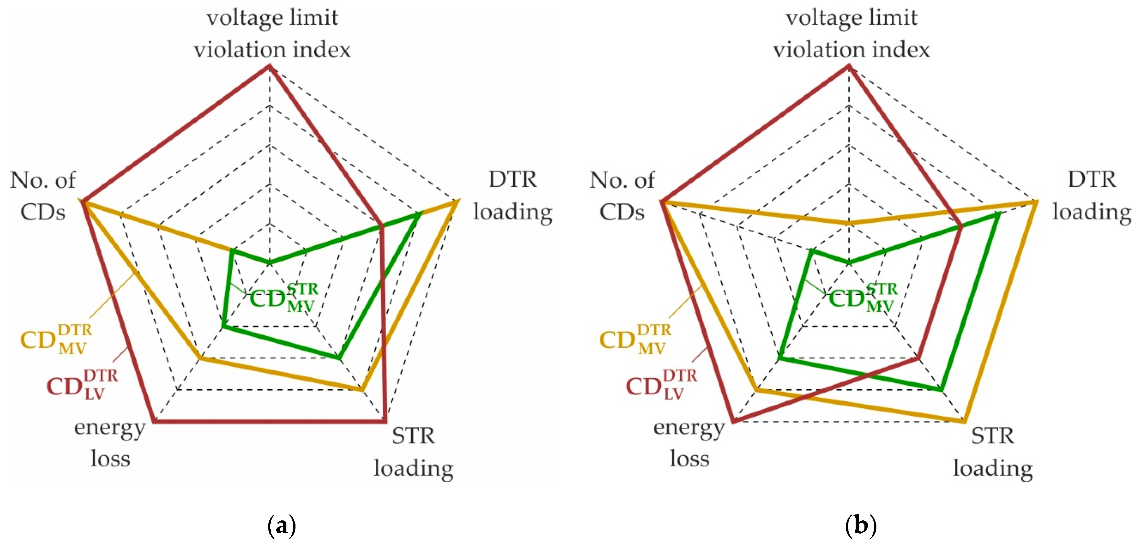
	${\mathbf{CD}}_{\mathbf{LV}}^{\mathbf{DTR}}$	0.8307	8.8536	31.9763	17.3888	22.3732	32

shows the relevant criteria used for the evaluation of different CD locations within the distribution grid with cable or overhead conductors in MV level. The energy loss, the average STR and DTR loadings, the average voltage limit violation index, and the energy exchange between MV_ and HV_link-grid are calculated according to Equations (A1)–(A5), Appendix B. Furthermore, one of the criteria applies to the number of compensation devices to be installed in each case.

The CD placement at the STR MV-bus bar supports the elimination of voltage limit violations in all cases, while the contrary is noticed when the CDs are placed on the DTR level. The placement of CDs on the MV side of DTRs provokes violations of the upper voltage limit in the case of overhead conductor type, ${\mathit{VI}}_{\mathit{avg}}=0.1484$. Meanwhile, when CDs are installed at the LV side of DTRs, limit violations appear in both cases, cable and overhead, with a ${\mathit{VI}}_{\mathit{avg}}$ of 0.0016 and 0.8307, respectively.

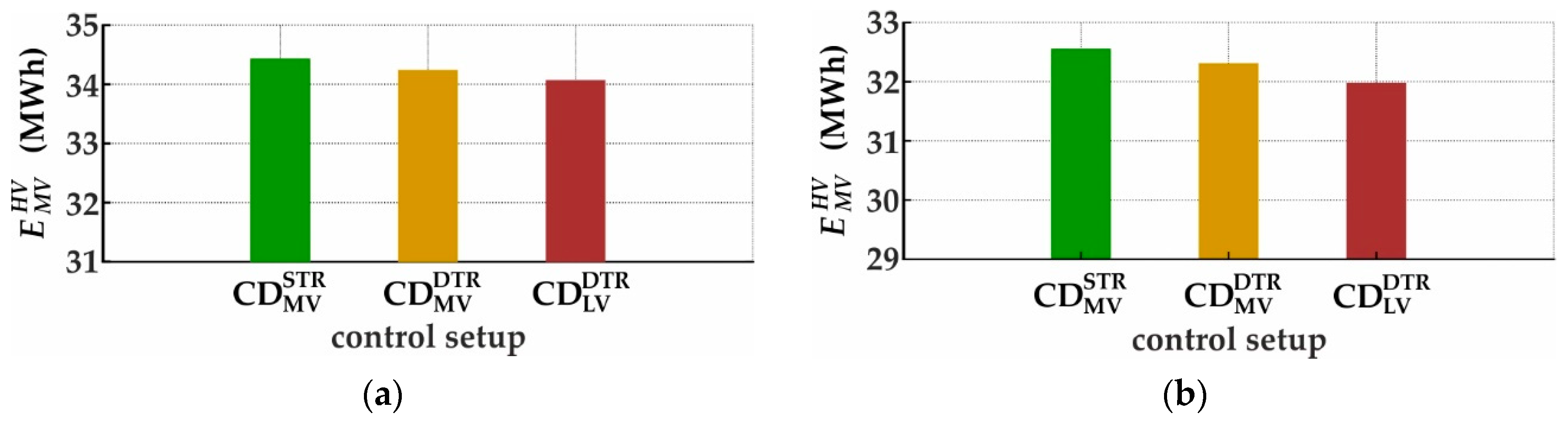
Regarding the active power loss over the all-time horizon, i.e., the active energy loss, a clear trend is observed for both conductor types in MV level: while the CD placement at the STR MV-bus bar causes the lowest energy losses of 6.5051 and 8.3320 MWh for cable and overhead conductors in MV level, respectively, the CD placement at DTRs’ LV-bus bars causes the highest ones of 7.2863 and 8.8536 MWh.

These results show that the compensation of the reactive power in distribution substation significantly deteriorates the effectiveness of L(U)-control, leading to very high losses and voltage limit violations in LV level.

The amount of active power flowing from MV_ to HV_link-grid over the all-time horizon, i.e., active energy exchange, depends on the placement of the CDs, Figure 14. Their placement in the supplying substation supports the maximum active energy exchange in all cases.

The STR and DTR loading depends on the active and reactive power flows. In our simulations the CD set on the MV-bus bar of the supplying substation completely compensates the reactive power exchange at all times. Thus, the average STR loading is exclusively provoked by the active power flow, achieving the minimum value of 17.9049% for the grid with cable conductors in MV level. In the case of overhead conductor type, the lowest value of 17.3888% is reached when the CDs are placed at the LV side of the DTRs. In this case, active and reactive energy flow through the STR, because the CDs compensate the reactive power in DTR level.

Anyhow, due to the reduced active energy exchange, Figure 14, the lowest STR loading value results for this control setup. The highest average STR loading of 19.0885% for the grid with cable conductors in MV level appears when CDs are installed at the DTRs’ LV-bus bars. In the case of overhead conductor type, the highest value of 17.4682% is reached when CDs are installed at MV-bus bars of the DTRs.

The number of CDs to install is very different. When placed at the STR MV-side, one CD per bus bar is required (or two CDs in double bus bar configurations), while the placement in the distribution substations normally requires as many CD devices as there are DTRs in place; which are in our case 32 CDs.

Figure 15 depicts a qualitative representation of the results given in Table 4.

The effectiveness of the solution depends on the size of the surface of the pentagon. The smaller the surface of the latter, the more effective is the solution. Results show that the distribution grid performs best when CDs are placed at the MV-bus bar of the STR.

3.2. Discussion

Results have shown that the VVC chain strategy supports the integration of rooftop PVs on a large scale. Figure 16 shows the most suitable setup of the VVC chain for a distribution grid with the highest PV share operated by one DSO. The VVC chain is designed with a minimum number of secondary and primary control units to reduce the associated investments and operating costs. Derived from Equation (1), the VVC chain in the Y-axis is presented by:

$$\begin{array}{c}{\mathrm{VVC}}^{\mathrm{Y}-\mathrm{axis}}{=\{\mathrm{VV}\mathbf{SC}}^{\mathrm{MV}}\left({\mathrm{volt}\mathbf{PC}}_{\mathrm{OLTC}}^{\mathrm{MV}}{,\mathrm{var}\mathbf{PC}}_{\mathrm{RD}}^{\mathrm{MV}}{,\mathrm{var}\mathbf{PC}}_{\mathrm{DG}}^{\mathrm{MV}}{,\mathrm{VV}\mathbf{SC}}_{\mathrm{ngb}}^{\mathrm{MV}}{,\mathrm{var}\mathbf{Cns}}_{\mathrm{MV}}^{\mathrm{HV}}\right){,\mathrm{var}\mathbf{LC}}_{\mathrm{L}\left(\mathrm{U}\right)}^{\mathrm{LV}},\hfill \\ {\mathrm{VV}\mathbf{SC}}^{\mathrm{CP}}\left({\mathrm{var}\mathbf{PC}}_{\mathrm{inv}}^{\mathrm{CP}}{,\mathrm{var}\mathbf{Cns}}_{\mathrm{CP}}^{\mathrm{LV}}=0\right)\}.\hfill \end{array}$$

(13)

Two grid-link types, i.e., MV_ and CP_grid-link, are designed in this case. For the LV level, no grid-link is designed for four reasons:

(a)

MV_ and LV_link-grids have the same operator and as a result they do not have external interfaces between each other [16];

(b)

No reactive power is exchanged between LV_link-grids and CPs because of the Q-autarky of the latter;

(c)

No distributed energy resources are foreseen to deliver reactive power to the LV_link-grids;

(d)

At each LV feeder with voltage limit violation potential is installed one locally controlled L(U).

The MV_grid-link includes a VVSC^MV that coordinates the Q-contribution of DGs, RDs and the neighbour grid-links with the voltage at the secondary side or OLTC position of the STR while respecting the reactive power constraints, ${\mathrm{var}\mathbf{Cns}}_{\mathrm{MV}}^{\mathrm{HV}}$, on the HV-MV intersection points and optimizing the network performance at the same time. The HV-MV intersection points correspond in many cases with TSO-DSO intersection points. ${\mathrm{var}\mathbf{Cns}}_{\mathrm{MV}}^{\mathrm{HV}}$ is dynamic and therefore needs to be discussed and defined through real-time TSO and DSO cooperation in order to achieve an optimal solution, in both, transmission and distribution grids.

Simulation results have shown that the uncontrolled reactive power flow provoked by the locally controlled units, ${\mathrm{var}\mathbf{LC}}_{\mathrm{L}\left(\mathrm{U}\right)}^{\mathrm{LV}}$, included in LV_link-grid is best compensated by the CD installed at the MV-bus bar of the STR. ${\mathrm{var}\mathbf{LC}}_{\mathrm{L}\left(\mathrm{U}\right)}^{\mathrm{LV}}$s, installed at the end of each LV lateral with voltage limit violation potential, keep the voltage below the upper limit during the PV production period.

The CP_grid-links have a ${\mathrm{VV}\mathbf{SC}}^{\mathrm{CP}}\left({\mathrm{var}\mathbf{PC}}_{\mathrm{inv}}^{\mathrm{CP}}{,\mathrm{var}\mathbf{Cns}}_{\mathrm{CP}}^{\mathrm{LV}}=0\right)$ that takes care to fully compensate the reactive power of the customer plant at all times. The interaction between the LV_link-grid and CPs in terms of reactive power is not existing and therefore no exchange of information between the DSO and the customers is required. Thus, the ICT challenge for the volt/var control is resolved at the LV level. The CPs inject or obtain exclusively active power into or from the LV_link-grid.

The VVSC^MV is practically realized in real time in the frame of the industrial project Central Volt/var control in Presence of Distributed Generation (ZUQDE, Salzburg, Austria) [29,30]. The distribution state estimator was realized in a MV grid of European type with a symmetrical balanced behaviour. The ${\mathrm{VV}\mathbf{SC}}^{\mathrm{MV}}\left({\mathrm{volt}\mathbf{PC}}_{\mathrm{OLTC}}^{\mathrm{MV}}{,\mathrm{var}\mathbf{PC}}_{\mathrm{DG}}^{\mathrm{MV}},\cos \mathsf{\phi }{\mathbf{Cns}}_{\mathrm{MV}}^{\mathrm{HV}}\right)$ was successfully realized in closed loop. This project has indicated that the implementation of the proposed VVC chain strategy has great potential to be realized on an industrial scale.

4. Conclusions

Due to the current trends in distribution grids, i.e., implementation of distributed generation with local volt/var control, the local voltage increases, the process of reactive power management throughout the power grid becomes very difficult and the information and communications technology (ICT) related challenge follows up. Therefore, solving the problem of voltage control and reactive power management is of utmost importance to utilities, as they may favor the large scale integration of distributed generation.

Results of this investigation have shown that the VVC chain strategy, which roots on LINK-based holistic architecture, supports the integration of rooftop PVs on a large scale. The inclusion of the L(U)+CP_Q-autarky control ensemble in the control chain eliminates the violation of the upper voltage limit at low voltage level, as well as the ICT challenges and social problems. The VVC chain is designed with a minimum number of secondary and primary control units to reduce the associated investments and operating costs. It consists of two volt/var secondary controls; one at medium voltage level (which also controls the TSO-DSO reactive power exchange), the other at the customer plant level. MV and LV grids have the best performance in terms of losses, loading of distribution and supplying transformers, number of installed compensation devices and active power production, when the compensation device is placed at the MV bus bar of supplying transformer.

One part of the VVC chain, VVSC^MV, is industrially realized in real time in another project. Nevertheless, the industrial implementation of the entire VVC chain is the next step to prove the practical relevance of the results of this study.

References

- Guterres, A. Secretary-General’s Remarks at High-Level Meeting on Climate and Sustainable Development, 28 March 2019; United Nations: New York, NY, USA, 2019; Available online: https://www.un.org/sg/en/content/sg/statement/2019-03-28/secretary-generals-remarks-high-level-meeting-climate-and-sustainable-development-delivered (accessed on 4 October 2019).
- Environmental Protection Agency. Distributed Generation of Electricity and Its Environmental Impacts. Available online: https://www.epa.gov/energy/distributed-generation-electricity-and-its-environmental-impacts (accessed on 4 October 2019).
- Eurelectric. Power Distribution in Europe: Facts and Figures. 2013. Available online: https://www3.eurelectric.org/media/113155/dso_report-web_final-2013-030-0764-01-e.pdf (accessed on 4 October 2019).
- Bollen, M.H.J.; Sannino, A. Voltage control with inverter-based distributed generation. IEEE Trans. Power Deliv. 2005, 20, 519–520. [Google Scholar]
- Demirok, E.; González, P.C.; Frederiksen, K.H.B.; Sera, D.; Rodriguez, P.; Teodorescu, R. Local reactive power control methods for overvoltage prevention of distributed solar inverters in low-voltage grids. IEEE J. Photovolt. 2011, 1, 174–182. [Google Scholar] [CrossRef]
- Caldon, R.; Coppo, M.; Turri, R. Distributed voltage control strategy for LV networks with inverter-interfaced generators. Electr. Power Syst. Res. 2014, 107, 85–92. [Google Scholar] [CrossRef]
- Bae, Y.; Vu, T.; Kim, R. Implemental Control Strategy for Grid Stabilization of Grid-Connected PV System Based on German Grid Code in Symmetrical Low-to-Medium Voltage Network. IEEE Trans. Energy Convers. 2013, 28, 619–631. [Google Scholar] [CrossRef]
- Esslinger, P.; Witzmann, R. Improving grid transmission capacity and voltage equality in low-voltage grids with a high proportion of distributed power plants. In Proceedings of the International Conference Smart Grid Clean Energy Technologies, Chengdu, China, 27–30 September 2011. [Google Scholar]
- Malekpour, A.R.; Pahwa, A. Reactive power and voltage control in distribution systems with photovoltaic generation. In Proceedings of the North American Power Symposium (NAPS), Champaign, IL, USA, 9–11 September 2012. [Google Scholar]
- Ciocia, A.; Boicea, V.A.; Chicco, G.; Leo, P.D.; Mazza, A.; Pons, E.; Spertino, F.; Hadj-Said, N. Voltage Control in Low-Voltage Grids Using Distributed Photovoltaic Converters and Centralized Devices. IEEE Trans. Ind. Appl. 2019, 55, 225–237. [Google Scholar] [CrossRef]
- NERC. Reliability Guideline: Reactive Power Planning. December 2016. Available online: https://www.nerc.com/comm/PC_Reliability_Guidelines_DL/Reliability%20Guideline%20-%20Reactive%20Power%20Planning.pdf (accessed on 4 October 2019).
- Chiang, H.D.; Wang, J.C.; Tong, J.; Darling, G. Optimal capacitor placement, replacement and control in large-scale unbalanced distribution systems: Modeling and a new formulation. IEEE Trans. Power Syst. 1995, 10, 356–362. [Google Scholar] [CrossRef]
- Lund, P. The Danish cell project—Part 1: Background and general approach. In Proceedings of the IEEE Power Engineering Society General Meeting, Tampa, Fl, USA, 24–28 June 2007. [Google Scholar]
- ETIP SNET. Holistic Architectures for Future Power Systems. 8 March 2019. Available online: https://www.etip-snet.eu/white-paper-holistic-architectures-future-power-systems/ (accessed on 4 October 2019).
- Ilo, A. The Energy Supply Chain Net. Energy Power Eng. 2013, 5, 384–390. [Google Scholar] [CrossRef] [Green Version]
- Ilo, A. Effects of the Reactive Power Injection on the Grid—The Rise of the Volt/var Interaction Chain. Smart Grid Renew. Energy 2016, 7, 217–232. [Google Scholar] [CrossRef]
- Ilo, A. Link—The Smart Grid Paradigm for a Secure Decentralized Operation Architecture. Electr. Power Syst. Res. 2016, 131, 116–125. [Google Scholar] [CrossRef]
- Ilo, A.; Schultis, D.-L. Low-voltage grid behaviour in the presence of concentrated var-sinks and var-compensated customers. Electr. Power Syst. Res. 2019, 171, 54–65. [Google Scholar] [CrossRef]
- Schultis, D.-L.; Ilo, A. A new Volt/var local control strategy in low-voltage grids in the context of the LINK-based holistic architecture. In Proceedings of the IEWT, Vienna, Austria, 13–15 February 2019. [Google Scholar]
- Schultis, D.-L.; Ilo, A.; Schirmer, C. Overall performance evaluation of reactive power control strategies in low voltage grids with high prosumer share. Electr. Power Syst. Res. 2019, 168, 336–349. [Google Scholar] [CrossRef]
- Schultis, D.-L. Comparison of Local Volt/var Control Strategies for PV Hosting Capacity Enhancement of Low Voltage Feeders. Energies 2019, 12, 1560. [Google Scholar] [CrossRef]
- Schirmer, C.; Ilo, A. The impact of the uncoordinated local control of decentralized generation on the reactive power margin. In System Operation and Control, Proceedings of the CIGRE Session 47, Paris, France, 26–31 August 2018; Cigre: Paris, France, 2018. [Google Scholar]
- Ilo, A.; Schultis, D.-L.; Schirmer, C. Effectiveness of Distributed vs. Concentrated Volt/Var Local Control Strategies in Low-Voltage Grids. Appl. Sci. 2018, 8, 1382. [Google Scholar] [CrossRef]
- Schultis, D.-L. Volt/Var Behaviour of Low Voltage Grid-Link in European Grid Type. Master’s Thesis, TU Wien, Viena, Austria, November 2017. [Google Scholar]
- E-Control, Technische und organisatorische Regeln für Betreiber und Benutzer von Netzen. TOR Erzeuger: Anschluss und Parallelbetrieb von Stromerzeugungsanlagen des Typs A und von Kleinsterzeugungsanlagen. Version 1.0. 2019. Available online: https://www.e-control.at/documents/1785851/1811582/TOR+Erzeuger+Typ+A+V1.0.pdf/6342d021-a5ce-3809-2ae5-28b78e26f04d?t=1562757767659 (accessed on 4 October 2019).
- Schultis, D.-L.; Ilo, A. Adaption of the Current Load Model to Consider Residential Customers Having Turned to LED Lighting. In Proceedings of the IEEE APPEEC, Macao, China, 1–4 December 2019. Accepted for Publication. [Google Scholar]
- Schultis, D.-L. Daily Load Profiles and ZIP Models of Current and New Residential Customers; Mendeley Data; Elsevier: Amsterdam, The Netherlands, 2019; Volume 1. [Google Scholar] [CrossRef]
- Schultis, D.-L.; Ilo, A. TUWien_LV_TestGrids; Mendeley Data; Elsevier: Amsterdam, The Netherlands, 2018; Volume 1. [Google Scholar] [CrossRef]
- ZUQDE-Project, Final Report. 2012. Available online: https://www.energieforschung.at/assets/project/final-report/ZUQDE.pdf (accessed on 4 October 2019).
- Ilo, A.; Schaffer, W.; Rieder, T.; Dzafic, I. Dynamische Optimierung der Verteilnetze—Closed loop Betriebergebnisse. In Proceedings of the VDE Kongress, Stuttgart, Germany, 5–6 November 2012. [Google Scholar]
Figure 1.
The generalized form of the volt/var control chain strategy implying the L(U)+Q-autarky control ensemble.
Figure 2.
Customer plant model: (a) structure; (b) load and production profiles.
Figure 3.
Simplified one-line diagram of the LV_link-grid model.
Figure 4.
Simplified one-line diagrams of the MV_link-grid models with different conductor types: (a) cable; (b) overhead line.
Figure 5.
Simplified form of the VVC chain strategy representing the setup without any var control.
Figure 6.
Simplified form of the VVC chain strategy representing the setup with L(U)-control and CP_Q-autarky.
Figure 7.
Simplified form of the VVC chain strategy representing the setup with L(U)-control, CP_Q-autarky and a CD at the STR MV-busbar.
Figure 8.
Simplified form of the VVC chain strategy representing the setup with L(U)-control, CP_Q-autarky and CDs at the DTRs’ MV-busbars.
Figure 9.
Simplified form of the VVC chain strategy representing the setup with L(U)-control, CP_Q-autarky and CDs at the DTRs’ LV-busbars.
Figure 10.
Voltage profile of the MV_link-grid with cable conductors and the backmost LV_link-grid at
Figure 11.
Behaviour of the distribution grid with cable conductors in MV level for a 24 h time horizon and different control strategies: (a) Q-consumption of L(U)s; (b) Q-contribution of CDs; (c) Q-exchange between HV_ and MV_link-grid; (d) active power losses; (e) STR loading; (f) mean DTR loading.
Figure 12.
Voltage profile of the MV_link-grid with overhead line conductors and the backmost LV_link-grid at .
Figure 13.
Behaviour of the distribution grid with overhead line conductors in MV level for a 24 h time horizon and different control strategies: (a) Q-consumption of L(U)s; (b) Q-contribution of CDs; (c) Q-exchange between HV_ and MV_link-grid; (d) active power losses; (e) STR loading; (f) mean DTR loading.
Figure 14.
Active energy exchange between MV_and HV_link-grid for different conductor types in MV level: (a) cable; (b) overhead line.
Figure 15.
Qualitative representation of the criteria used for the evaluation of various CD placements on a distribution grid with different conductor types in MV level: (a) cable; (b) overhead line.
Figure 16.
The most suitable setup of the VVC chain for a distribution grid with the highest PV share operated by one DSO.