Article

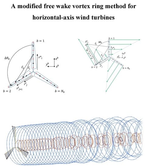
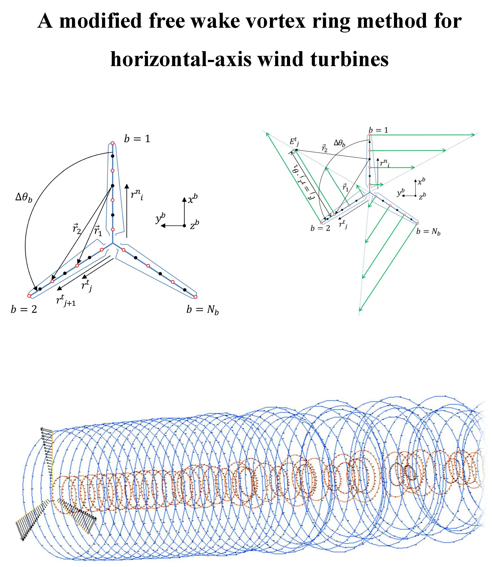
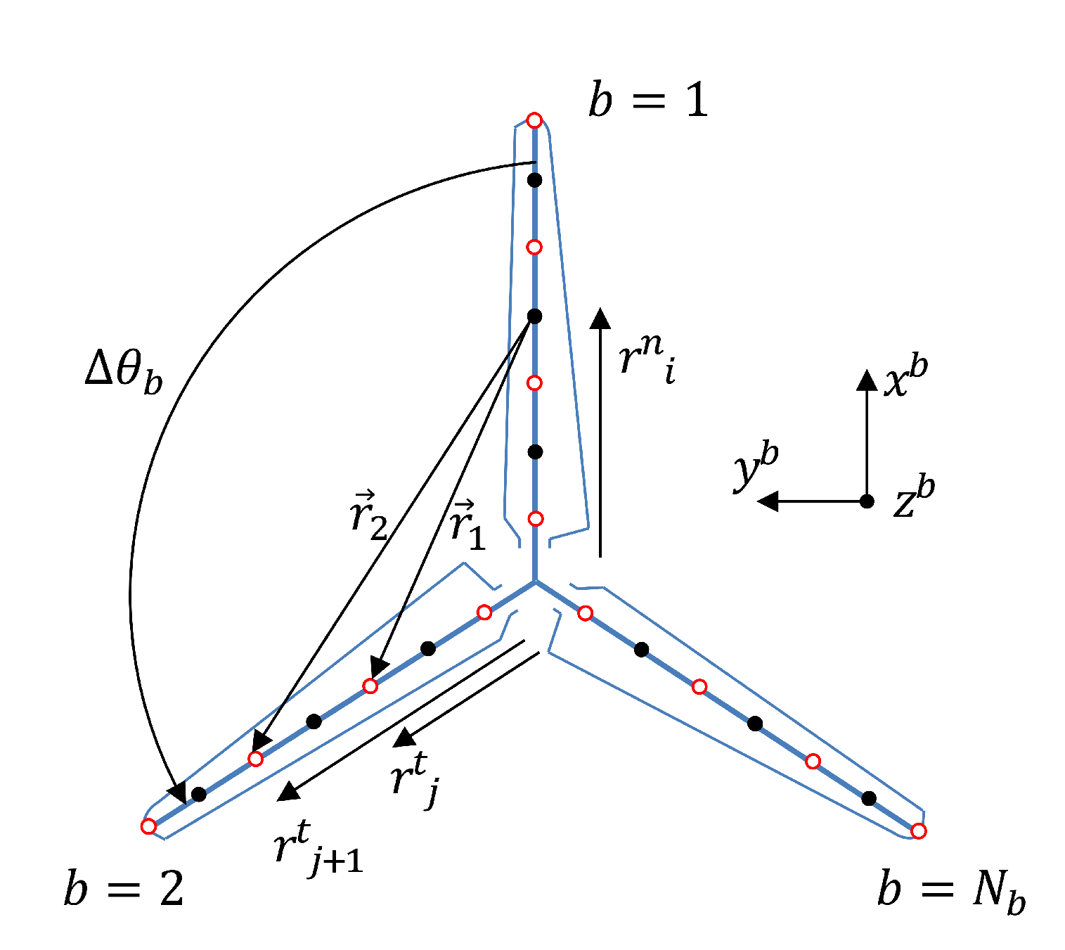
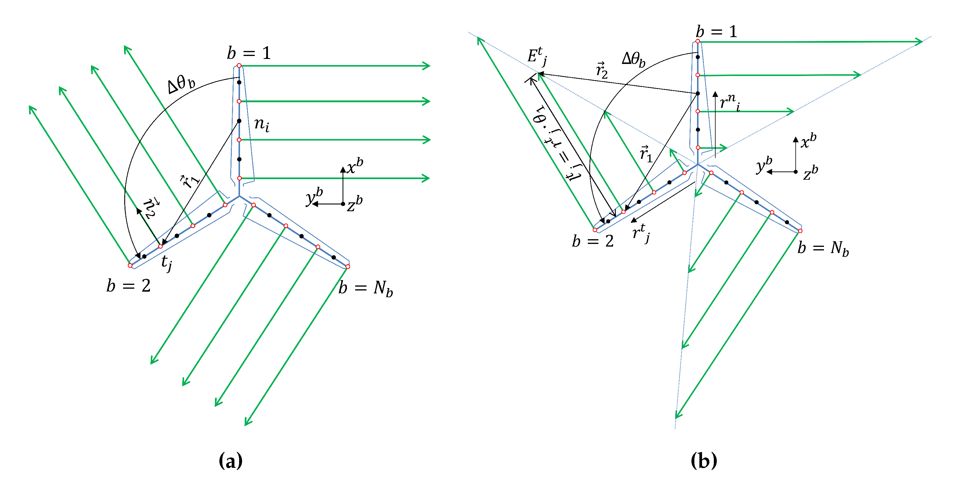
A Modified Free Wake Vortex Ring Method for Horizontal-Axis Wind Turbines

1
Faculty of Aerospace Engineering, Delft University of Technology, Kluyverweg 1, 2629 HS Delft, The Netherlands
2
Wind Energy Group, Shanghai Electric Group Company Limited, Shanghai 200233, China
*
Author to whom correspondence should be addressed.
Energies 2019, 12(20), 3900; https://doi.org/10.3390/en12203900
Submission received: 5 August 2019 / Revised: 7 October 2019 / Accepted: 10 October 2019 / Published: 15 October 2019
(This article belongs to the Special Issue Recent Advances in Aerodynamics of Wind Turbines)

Abstract

:
A modified free-wake vortex ring model is proposed to compute the dynamics of a floating horizontal-axis wind turbine, which is divided into two parts. The near wake model uses a blade bound vortex model and trailed vortex model, which is developed based on vortex filament method with straight lifting lines assumption. By contrast, the far wake model is based on the vortex ring method. The proposed model is a good compromise between accuracy and computational cost, for example when compared with more complex vortex methods. The present model is used to assess the influence of floating platform motions on the performance of a horizontal-axis wind turbine rotor. The results are validated on the 5 MW NREL rotor and compared with other aerodynamic models for the same rotor subjected to different platform motions. The results show that the proposed method is reliable. In addition, the proposed method is less time consuming and has similar accuracy when comparing with more advanced vortex based methods.

Graphical Abstract

1. Introduction

The unsteady aerodynamic loads experienced by floating offshore wind turbines (FOWTs) can be significantly different from those of bottom-fixed wind turbines [1]. Simulation tools that can accurately evaluate the relationship between the aerodynamic loads on the rotor and the platform motion are required especially for off-design conditions or novel concepts. Thus far, the available aero-hydro coupled analysis tools are almost exclusively based on the blade element momentum (BEM) theory, which describes the steady state behavior of a wind turbine but is unsuitable when the rotor interacts with its own wake, as is the case for FOWTs. An alternative is to use computational fluid dynamics (CFD) models that describe the flow physics around the rotor with higher fidelity. However, they are computationally expensive when dealing with the fully-coupled dynamics of FOWTs. Another approach, which is more accurate than momentum theory and less costly than CFD, is the so-called vortex methods. Vorticity-based methods have a number of different formulations, ranging from simple analytical models to more advanced numerical methods [2]. In addition, the computational cost of vortex models depends on the number of vortex elements and the interaction between them, ranging from relatively computationally less expensive models to more expensive ones [3,4]. Since the rotating wind turbines generate bounded circulations on the blades and release vorticity into the wake, the vortex based methods are naturally suitable for the simulation of wind turbine aerodynamics. The blade vorticity is assumed to be concentrated on lifting lines, with distributed vortex strengths representing the bound circulation, which convect to the wake as shed and trailed vorticity. The shed vorticity is the vorticity emitted in the wake due to time change of the bound circulation, while the trailed vorticity results from the spanwise change of bound circulation [2]. Within the scope of simplified vorticity models for rotors, the wake flow can be represented by vortex filaments such as the free wake vortex filament (FWVF) method of [5], vortex particles such as the nonlinear vortex lattice method (NVLM) method of [6], or a vortex ring model. As for the vortex ring methods, the wake is modeled with vortex rings with constant circulations determined by the aerodynamic loads on the rotor. Each vortex ring induces velocity on both the rotor and the other rings in the wake. The radius and spacing of the rings are time-varying, which is the so-called free wake vortex ring method. In this method, the analytical solution of the induced velocity of an axisymmetric vortex ring derived from Biot–Savart law [7,8] is used to calculate the induced velocities in the wake as well as on the rotor, which reduces computation cost while retaining the basic physical properties in the wake.
The simplest vortex ring methods available in the literature represent the rotor with an actuator disc, while the wake is modeled as vortex rings released at the tip of the rotor [9,10,11]. These models were used to calculate unsteady aerodynamic loads on both fixed and moving rotors. However, some aerodynamic features such as angle of attack, and lift and drag forces on the rotor could not be accurately reproduced due to the limitations associated with the actuator disc concept. A modeling method that represents the rotor blades with lifting lines, the near wake as a series of straight vortex lines and the far wake by vortex rings was initially suggested by Miller [12], relating the blade bound vortex strength with the vortex ring strength in the wake. In that case, the rotor loads were also dependent on the induced velocities from the vortex rings. Afjeh [13] and de Vaal [14,15] adapted and improved this method to the modeling of wind turbines, and good agreement was achieved when comparing the numerical results with measurement data.
The proposed free wake vortex ring method (FWVR) is based on the work of de Vaal [15] which is an aerodynamic model of a horizontal-axis wind turbine. It combines the Kutta–Joukowski lift theorem with the blade element theory, which can accurately and effectively predict the blade load using the time-evolution of the induced velocities. It splits the wake into near wake and far wake, leading to more realistic velocities on the blade and in the far-field. However, the application of de Vaal’s original method [15] can be challenging for some working states, for example the case of small or negative angles of attack at low wind speeds, or blade pitching motions at high wind speeds. In this paper, we present a few modifications of the original method to overcome these challenges. First, the propagation process of the vortex rings is modified and different nonlinear iteration methods are tested to solve the blade bound vortex strengths. Second, the near-wake trailed vortex model uses finite length of vortex segments instead of semi-infinite vortex lines, which is physically more realistic.
The proposed free wake vortex model was validated by analyzing the aerodynamic parameters on the NREL 5 MW wind turbine with both fixed-bottom and different types of platforms foundations, i.e., ITI barge, OC3-Hywind spar-buoy (OHS), and tension leg platform (TLP). The results were compared with those obtained from BEM theory, RANS method of [16] and two vortex based aerodynamic models—the FWVF method of [5] and the NVLM method of [6].
The paper is organized as follows. The theory of the modified free wake vortex ring method is described in Section 2. The numerical modeling method is described and validated in Section 3. The computational time evaluation is shown in Section 4. The wind turbine aerodynamic analysis is shown in Section 5. Finally, conclusions are drawn in Section 6.

2. Vortex Ring Theory

The proposed free wake vortex ring method consists of two parts: the near wake model and the far wake model. The induced velocities of the near wake model are calculated based on Biot–Savart law, as described in Section 2.1. To keep a low computational cost, the far wake model is represented by the axisymmetric vortex rings, as introduced in Section 2.2.

2.1. Velocity Induced by a Vortex Filament

The velocity V P induced by a vortex filament with a constant strength Γ in the field at a point P can be expressed by Biot–Savart law as [17]
V P = Γ 4 π C ( q ) r P r q | r P r q | 3 × r q q d q ,
where C ( q ) is the parametric curve which describes the path of the vortex filament, r P is the position vector of the point P, r q is the position vector of a point Q on the filament, r = r P r q is the vector pointing from point Q to point P, and r q q is the partial derivative of r q with respect to the filament parameter. In Equation (1), the kernel of Biot–Savart operator is identified as
K ( r ) = 1 4 π r | r | 3 ,
which singular when the point P is on the vortex filament C ( q ) . To avoid the singularity, a smoothing method proposed by Hoydonck et al. [18] is used, which replaces K ( r ) with K σ ( r ) , defined as
K σ ( r ) = g ( σ ) | r | 3 r ,
where σ is the non-dimensionalized length between the point P and a point on the filament, and g ( σ ) is a three-dimensional velocity smoothing function [18]. Here, the Rosenhead–Moore velocity smoothing function is used, i.e.,
g ( σ ) = σ 3 4 π ( σ 2 + 1 ) 3 2 .
This leads to the following induction velocity,
V P = Γ C ( q ) K σ ( r ) × r q q d q .
Considering a straight line vortex filament, the parametric curve of the filament is given by C ( q ) = x 1 + q ( x 2 x 1 ) , with 0 q 1 . Thus, the desingularized kernel K σ ( r ) can be expressed as
K σ ( r ) = x P C ( q ) 4 π ( | x P C ( q ) | 2 + r c 2 ) 3 2 = x P ( 1 q ) x 1 + q x 2 4 π ( | x P ( 1 q ) x 1 + q x 2 | 2 + r c 2 ) 3 2 ,
where r c is the vortex core radius. Accordingly, the induced velocity V P can be expressed as
V P = Γ 0 1 x P ( 1 q ) x 1 + q x 2 4 π ( | x P ( 1 q ) x 1 + q x 2 | 2 + r c 2 ) 3 2 × ( x 2 x 1 ) d q .
When the point x 2 extends to infinity, the straight line vortex filament becomes a semi-infinite line. In this case, the upper limit of q = q ˜ extends to infinity, and the induced velocity V P becomes
V P = Γ lim q ˜ f ( q ) ,
f ( q ) = 0 q ˜ x P ( 1 q ) x 1 + q x 2 4 π ( | x P ( 1 q ) x 1 + q x 2 | 2 + r c 2 ) 3 2 × ( x 2 x 1 ) d q .

2.2. Velocity Induced by an Axis-Symmetric Vortex Ring

Considering an ideal vortex ring with radius R, as shown in Figure 1, its parametric curve C ( χ ) with the angle χ as the parameterization parameter can be expressed as
C ( χ ) = R ( cos χ , sin χ , 0 ) , χ [ 0 , 2 π ] .
In the local vortex ring coordinate frame x y z of an axis-symmetric vortex ring, the coordinates of P are ( x P , 0 , z P ) and C ( χ ) is located in the x y -plane, which centered at the origin of the z -axis. Thus, Taking the notation x P = η R and z P = ζ R , we have
r ( χ ) = R ( cos χ , sin χ , 0 ) ,
r P = R ( η , 0 , ζ ) , η ( 0 , + ) , ζ ( , + ) .
The displacement vector r is thus given by
r = r P r ( χ ) = R ( η cos χ , sin χ , ζ ) .
The vortex ring induced velocity at P is obtained by substituting the above equations into Equation (5), which yields:
V = Γ 4 π R 0 2 π ( ζ cos χ , ζ sin χ , 1 η cos χ ) ( 1 + η 2 + ζ 2 + σ c 2 2 η cos χ ) 3 2 d χ ,
where σ c = r c / R is the non-dimensional vortex core radius; a constant value of 0.0116 is taken where the self induced velocity agree with ring-center velocity [15]. An analytical result of this integral has been derived as [7,8]
V x = Γ 2 π R C 0 K ( m ) + 1 + η 2 + ζ 2 C 1 2 E ( m ) ζ η ,
V z = Γ 2 π R C 0 K ( m ) + 1 η 2 ζ 2 C 1 2 E ( m ) ,
with
C 0 2 = 1 + 2 η + η 2 + ζ 2 + σ c 2 ,
C 1 2 = 1 2 η + η 2 + ζ 2 + σ c 2 ,
and the functions K ( m ) and E ( m ) being the first and second types of complete elliptic integrals, respectively, with m defined as:
m = 4 η C 0 2 .

3. Numerical Model

As explained in Section 2, the present free wake vortex ring model consists of two parts: the near wake model and the far wake model. The near wake model includes the blade bound vortex model and the trailed vortex model, which are both represented by vortex line segments. The velocities induced by these vortex lines are calculated based on Biot–Savart law, as described in Section 2.1. By contrast, the velocity induced by the far wake model is given by Equations (15) and (16). Section 3.1 gives more insights into the discretization of blades using vortex elements, while Section 3.2 discusses how the far wake model is implemented and how vortex rings propagate in the wake.

3.1. Near Wake Models

3.1.1. Blade Bound Vortex Model

Figure 2 illustrates the blade bound vortex model for a rotor of N b = 3 blades with straight lifting lines assumption. Each blade is discretized with a series of vortex line segments. The radial endpoints on the vortex segments are denoted by r j t , while the control points are denoted by r i n , where r i n = ( r j t + r j + 1 t ) / 2 ( i = 1 , , N and j = 1 , , N + 1 ), N being the number of vortex segments. A local blade coordinate system x b y b z b is defined as right-handed and centered at the rotor root. The x b -axis is along the pitch axis and pointing towards the tip of the blade; the y b -axis points to the trailing edge of blade and is parallel to the chord line at the zero-twist blade section; and the z b -axis is orthogonal to both x b and y b . In the local blade coordinate system of a blade b, the rotor lies in the x b y b -plane, as shown in Figure 2. The coordinates of a control point n i and an endpoint t j are then expressed as
n i = 0 r i n 0 , t j = cos Δ θ b sin Δ θ b 0 sin Δ θ b cos Δ θ b 0 0 0 1 0 r j t 0 ,
where Δ θ b = ( b i b ) 2 π / N b is the angle between blade b i and blade b. Assuming x P = n i , x 1 = t 1 and x 2 = t 2 , and substituting Equation (20) into Equation (7), it can be found that the velocity induced by the segment x 1 x 2 at the control point n i equals zero in both the x b -direction and the y b -direction, and in the z b -direction is equal to
V i j z b = Γ j b r i n sin Δ θ b r 2 ( r j t r i n cos Δ θ b ) r 1 ( r j + 1 t r i n cos Δ θ b ) 4 π r 1 r 2 r c 2 + r i n 2 ( r i n cos Δ θ b ) 2 = A i j b Γ j b ,
where A i j b is the influence coefficient which only depends on the geometry and discretization of the rotor, and r 1 and r 2 are the lengths of the vectors x 1 x P and x 2 x P , respectively, i.e.,
r 1 = r c 2 + r i n 2 + r j t 2 2 r i n cos Δ θ b ,
r 2 = r c 2 + r i n 2 + r j + 1 t 2 2 r i n cos Δ θ b .
The total induced velocity at a control point n i is the sum of the influences of all the bound vortex segments on all N b blades, which can be expressed as
V i z b = b = 1 N b j = 1 N V i j z b = b = 1 N b j = 1 N A i j b Γ j b .
Considering that the rotor is axis-symmetric and that all the blades’ geometry and discretization are identical, the total induced velocity at all N control points on a blade b can be simplified as
V z b = b = 1 N b A b Γ b ,
where A b is the matrix of influence coefficients of the blade bound vortex model.

3.1.2. Trailed Vortex Model

In this section, a finite length vortex line model is introduced as opposed to the semi-infinite vortex line model proposed by de Vaal [14], as shown in Figure 3a. A local blade coordinate system x b y b z b is used, where the rotor lies in the x b y b -plane and the blade b lies along the x b -axis. In the present model, the trailed vortex line begins from an endpoint r j t on a blade and extends to a finite length l j t as defined in Equation (26) in the direction normal to the blade in the x b y b -plane.
l j t = r j t θ t ,
which equals to the arc length of r j t times the angle θ t swept, where θ t is an input parameter.
The induced velocity at the control point n i on blade b can be determined using Equation (7). The coordinates of x P and x 1 are both given by Equation (20), while the coordinates of x 2 can be written as
x 2 = cos Δ θ b sin Δ θ b 0 sin Δ θ b cos Δ θ b 0 0 0 1 r j t θ 1 r j t 0 .
Substituting Equations (20) and (27) into Equation (7), evaluating the integral and simplifying, the velocity induced by x 1 x 2 at n i is derived as
V i j z t = Δ Γ j t ( r j t r i n cos Δ θ b ) r 2 r i n sin Δ θ b r 1 ( r j t r i n sin Δ θ b ) 4 π r 1 r 2 r c 2 + r j t 2 2 r i n r j t cos Δ θ b ( r i n cos Δ θ b ) 2 = A i j t Δ Γ j t ,
where r 1 and r 2 are the lengths of the vectors x 1 x P and x 2 x P , respectively, where r 1 is given in Equation (22) and r 2 can be defined as
r 2 = r c 2 + r i n 2 + r j t 2 ( 1 + θ 1 2 ) 2 r i n r j t ( cos Δ θ b + θ 1 sin Δ θ b ) .
The total trailed model induced velocity at a control point n i is the sum of the induce of all the N + 1 trailing vortex segments on all N b blades, which can be expressed as
V i z t = b = 1 N b j = 1 N + 1 V i j z t = b = 1 N b j = 1 N + 1 A i j t Δ Γ j t ,
which can be rewritten as
V z t = b = 1 N b A t Δ Γ t ,
where A t is the matrix of influence coefficients of the trailed vortex model.

3.1.3. Total Induced Velocity of the Near Wake
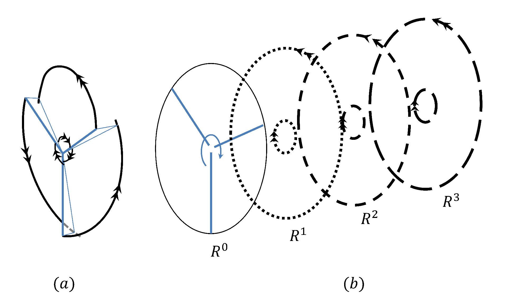
The total near wake induced velocity V n w is the sum up of the components of the blade bound vortex model in Equation (25) and the trailed vortex model in Equation (31). With non-zero values only in the z b -direction, V n w is given in Equation (32), which only depends on the rotor geometry.
V n w = b = 1 N b A b Γ b + A t Δ Γ t .

3.2. Far Wake Model

The far wake model is formulated based on the assumption that the spiral vortices in the wake can be represented by a series of vortex rings, as illustrated in Figure 4. When all the blades together sweep a full revolution, a pair of new vortex rings R 1 is shed into the wake, the outer ring being shed from the outboard of the rotor and the inner ring being shed from the inboard of the rotor disc. The computation of the far wake induced velocity V P f w at a point P with N R pairs of vortex rings is given in Equation (33), with the theory as described in Section 2.2.
V P f w = k = 1 N R V i n , k + k = 1 N R V o u t , k ,
where V i n , k is the induced by the kth inner ring and V o u t , k is induced by the outer ring.

The Propagation of Vortex Ring

The far wake model is time-dependent, where two time scales are considered: (i) the time step for the vortex shedding is Δ T = T P / N b , where T P is the period of the rotor rotation; and (ii) the time step used to compute the vortex rings propagation is defined as Δ t = Δ T / n c s t , where n c s t is a constant integer. The calculation of the propagation is a cyclic process which involves three steps per Δ t at a time t:
  • Identify the control points on the vortex rings and calculate the velocities (induced velocity and free stream velocity) on all the control points.
  • Calculate the position of the control points both on the rotor and in the wake. The control points in the wake is given by Euler’s equation assuming an incompressible and inviscid fluid, as
    S ( t + Δ t ) = S ( t ) + V Δ t ,
    where V is the speed of a control point in the global coordinate system.
  • Update the position of the vortex rings based on the control points determined in step 2.
The geometry parameters that describe a vortex ring k are collected into the variable S k , as
S k = x O , k y O , k z O , k R k χ k β k γ k k = 1 , , N R ,
where O k is the vortex ring center, R k is the ring radius, and γ k , χ k and β k are, respectively, roll, pitch and yaw angles, all of which being functions of time. Here, we consider a local inertial coordinate system x ^ y ^ z ^ by translating the origin of the global coordinate coincide with that of a vortex ring k. At the upright position, when the ring lies in the x ^ y ^ -plane, χ k and β k are both zero, and when it rotates anti-clockwise around the corresponding axis according to the right-hand law, the value of the angle is defined as positive. Due to the rotational invariance property of the ring, the roll angle γ k around the z ^ -axis has no influence on the position of the ring itself but represents the azimuthal angle between the ring and the control point. In the following, the method to determine these parameters is introduced.
Let us define a local vortex ring coordinate system x y z by giving the local inertial coordinate system x ^ y ^ z ^ a pitch angle of χ k and then a yaw angle of β k , so that the vortex ring lies in the x y -plane. A vortex ring in the wake is represented by a series of control points distributed on the ring with the azimuthal angle Δ θ . With N c control points on a vortex ring, Δ θ = 2 π / N c . Thus, the coordinate X i , k = ( x i , k , y i , k , z i , k ) of a control point i on a ring k in the local vortex ring coordinate system is given as
x i , k = R k sin [ Δ θ ( i 1 ) ] y i , k = R k cos [ Δ θ ( i 1 ) ] z i , k = 0 i = 1 , , N c , k = 1 , , N R .
which need to be expressed in the global coordinate frame denoted by X i , k ( t Δ t ) . At a time step t, the position of the control point denoted by X i , k ( t ) is determined by Equation (34) as:
X i , k ( t ) = X i , k ( t Δ t ) + V i , k Δ t .
Since the control points move independently, the new positions of the control points may no longer form an exact circle. This discrepancy is however very small if the time step Δ t is small enough. Nevertheless, a new vortex ring with the geometry parameters as shown in Equation (35) needs to be determined by the updated position of the azimuthal control points. Firstly, the vortex ring origin coordinate O k can be expressed by taking the average of the coordinates of all the control points as
O k = 1 N c i = 1 N c X i , k = 1 N c i = 1 N c ( x i , k , y i , k , z i , k ) .
Next, the vortex ring radius R k are determined by taking the average length of the segments s i , O from each control point i to the center of the ring O k as
R k = 1 N c i = 1 N c ( x i , k x O , k ) 2 + ( y i , k y O , k ) 2 + ( z i , k z O , k ) 2 .

3.3. Characteristics of the First Rings Shed in the Wake

After a certain distance behind the rotor, the trailed vortex segments of the near wake roll up into two concentrated vortex rings in the far wake. The initial size and vortex strength of the vortex rings are defined in this section. The algorithms of the roll-up process is based on the momentum conservation theory [14,19]. The location of the maximum blade bound vortex strength Γ m a x is used to define the inner and outer rings. In particular, the near wake trailing vortices from Γ m a x to the tip of the blade are roll up into an outer ring and from Γ m a x to the root of the blade roll up into an inner ring. The vortex strength of the roll up vortex ring equals to the summation of the vortex strengths of the trailing vortices from which it is formed. The vortex ring strengths Γ ¯ i n b and Γ ¯ o u t b as well as the vortex ring radii r ¯ i n b and r ¯ o u t b on blade b can be expressed as
Γ ¯ i n b = r 1 r 2 d Γ b d r d r = n = 1 n m a x Δ Γ n t ,
r ¯ i n b = 1 Γ ¯ i n b r 1 r 2 r d Γ b d r d r = 1 Γ ¯ i n b n = 1 n m a x r n Δ Γ n t ,
Γ ¯ o u t b = r 1 r 2 d Γ b d r d r = n = n m a x + 1 N + 1 Δ Γ n t ,
r ¯ o u t b = 1 Γ ¯ o u t b r 1 r 2 r d Γ b d r d r = 1 Γ ¯ o u t b n = n m a x + 1 N + 1 r n Δ Γ n t .
The concentrated vortex strength and radius of the inner and outer ring are defined as an average of the vortex strengths and radii calculated from each blade, that is
Γ ¯ o u t = 1 N b b = 1 N b r ¯ o u t b , Γ ¯ i n = 1 N b b = 1 N b r ¯ i n b ,
r ¯ o u t = 1 N b b = 1 N b r ¯ o u t b , r ¯ i n = 1 N b b = 1 N b r ¯ i n b .

3.4. Strength of the Blade Bound Vortex

Based on the discussion above, it can be seen that both the trailing vortex strengths and the far wake vortex ring strengths are determined by the distribution of blade bound vortex strengths. Once the blade bound vortex strengths are known, the near wake induced velocity at any point of the rotor can be determined by Equation (32) and the far wake vortex ring strengths are determined at the roll-up processes and with no change during their convection in the wake. Thus, the blade bound vortex strengths need to be determined as a prerequisite. A method to calculate the blade bound vortex strengths based on the Kutta–Joukowski lift theorem and the blade element theory is discussed below.

3.4.1. Kutta–Joukowski Lift Theorem

The Kutta–Joukowski lift theorem as introduced by Phillips [20] is adopted to solve the blade bound vortex strength. Based on this theory, the lift force d F l acting on a vortex segment d l can be calculated by the product of the air density ρ , the bound vortex strength Γ b on the segment, and the relative wind velocity V , as
d F l = ρ Γ b V × d l ,
where V includes the contribution from the free stream V , the rotor rotation V Ω , the near wake induced velocity V n w , and the far wake induced velocity V f w , as well as the motion of the platform V p in the case of a floating offshore wind turbine. V has three components in the blade coordinate system as V x b in the x b -direction, which is along the pitch axis towards the tip of the blade, and V y b and V z b lie in the blade section and normal to the blade pitch axis, which can be written as
V = V + V Ω + V n w + V f w + V p = V x b V y b V z b ,
Substituting Equation (47) into Equation (46), and given that the x b -axis is parallel to d l , it is found that only the V y b and V z b components contribute to the lifting force acting on the blade. Thus, Equation (46) can be rewritten as
d F l = ρ Γ b V n × d l ,
where V n is the velocity vector that has only the V y b and V z b components, i.e.,
V n = 0 V y b V z b .

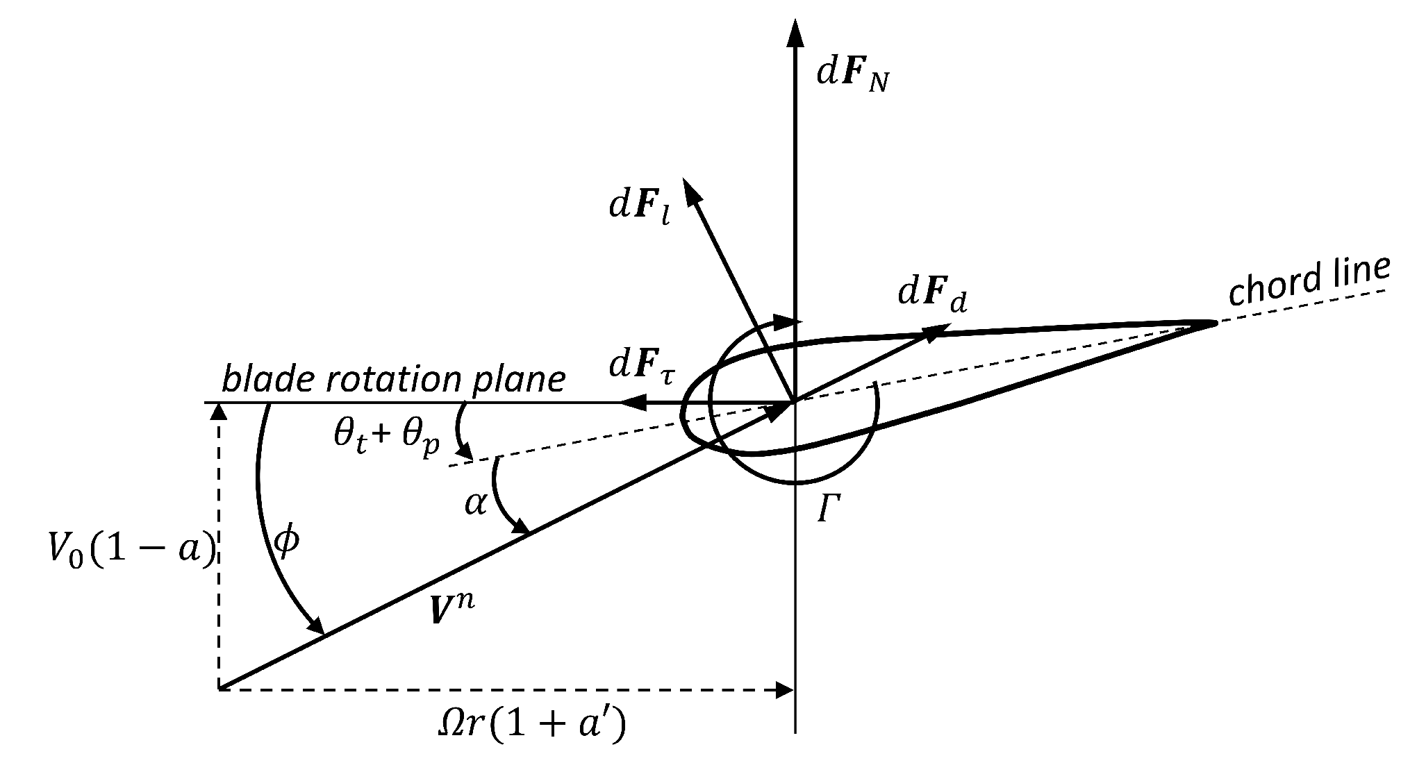
3.4.2. Blade Element Force

The lift force on a blade segment can also be calculated from the airfoil properties of the segment, as indicated in Figure 5. The lift force can be expressed as
d F l = 1 2 ρ V n 2 C l c d l ,
where V n is defined in Equation (49), c is the chord length, and C l is the lift coefficient obtained by means of tabulated aerodynamic parameters (the tabulated data are taken from the NREL certification cases of FAST: https://nwtc.nrel.gov/FAST8) of the airfoil with a given α , which is calculated as
α = ϕ ( θ t + θ p ) ,
where θ t is the twist angle, θ p is the collective pitch angle, and the angle of relative wind ϕ is the angle between the wind velocity V n and the plane of the rotor disc, which can be expressed as
ϕ = t a n 1 V 0 ( 1 a ) Ω r ( 1 + a ) .
In Equation (52), Ω is the rotor angular speed, a is the axial induction factor and a is the angular induction factor. Similar to the lift force, the drag force d F d is calculated from the tabulated C d and α , leading to
d F d = 1 2 ρ V n 2 C d c d l .
Based on the discussion above, it is found that both Equations (48) and (50) express the lift force of the blade segment. Thus, by equating them for a blade section i, the following relation is obtained
Γ i b | V i n ( Γ j ) × d l i | 1 2 | V i n ( Γ j ) | 2 C l ( α i ) c i d l i = 0 .
For each blade section i = 1 , , N b · N , an equation similar to Equation (54) can be set up, where j is the number of the vortex ring. For all N b · N blade sections, a system of N b · N non-linear equations are obtained and solved for N b · N unknown values of the bound vortex strength Γ i b . Different methods can be used to solve the resulting set of non-linear equations. The trust-region methods are used here, which proved to be more stable and converge more rapidly than Newton–Raphson methods, especially for small and negative angles of attacks. Accordingly, the rotor thrust F T is expressed as
F T = b = 1 N b j = 1 N d F N = b = 1 N b j = 1 N d F l cos ϕ + d F d sin ϕ .

4. Simulation Description

This simplified free wake vortex model aims at finding a compromise between physical accuracy and low computational cost. In this section, we compare the computational cost of the present method with other methods available in the literature. Table 1 shows the methods under consideration with computational cost and modeling capability: blade element momentum theory (BEM), actuator disc with free wake vortex ring model (AFWRV) of [10,11], the present free wake vortex ring model (FWVR), and two more advanced vortex methods—the free wake vortex filament (FWVF) method of [5] and the nonlinear vortex lattice method (NVLM) method of [6].
In Table 1, N b is the number of rotor blades, N θ is the number of time steps per rotor rotation and N Ω is the number of rotor rotation to be simulated. N θ N Ω represents the total number of time steps. C b represents the time cost of evaluating the induced velocity at a point in the field with BEM, C a , C r , C f and C m represent the time cost of evaluating the induced velocity of a vortex element (vortex rings or vortex filaments) at a point in the field with AFWVR, FWVR, FWVF and NVLM, respectively. Whether the blades are modeled or not, all four methods are evaluated with the same number of control points on the rotor and with the same number of time steps.
For the BEM theory, the number of control points are constant and each point is considered independently. Thus, the computational time has a linear relationship with the number of time steps, which is the fastest method for aerodynamic simulations. C b involves the iterative solution of BEM equations and some analytical corrections, such as Prandtl tip-loss, Prandtl hub-loss, and Pitt and Peters skewed-wake corrections when needed.
By contrast, the solution of the other four vortex methods mainly includes two parts: the calculation of the vortex element strength and the calculation of the induced velocity including self-induced velocities and mutually induced velocities. The equations need to be solved increases with the increase of vortex elements (being vortex rings or vortex filaments) in the wake.
The vortex ring strength of AFWVR is directly determined from a prescribed thrust coefficient C t [10], where the computational time is negligible. By contrast, the FWVR and FWVF methods determine the blade bound vortex strength by iteratively solving the equations based on the 3D vortex lifting law and the blade element theory with tabulated data of lift coefficient C l , and then the vortex strengths are distributed to the new generated vortex rings or vortex filaments in the wake. The computational times to determine the vortex strengths for FWVR, FWVF and NVLM methods at each time step are identical and denoted by C Γ . Since C Γ and C b are both iterative processes with the same number of equations, they are the same order of magnitude.
The computational times for evaluating the induced velocities of FWVR and FWVF are given in [14,21]. Since the number of vortex filaments is N θ times the number of vortex rings, the number of induced velocities that need to be calculated at each time step for FWVR is also N θ times that of FWVF. Since AFWVR has the same number of control points and vortex rings as FWVR, the number of induced velocities that needs to be calculated is the same. C a involves the analytical solution of a vortex ring induced velocity, which includes the evaluation of the elliptic integrals of the first and second kind. C r involves the same calculation as C a as well as the analytical solutions of near wake induced velocities at the rotor points where the time cost is very small. Thus, C r is approximately equal to C a . C f involves the solving of the trigonometry functions based on Biot–Savart law, and C m involves the solving of Biot–Savart kernel functions. Thus, C f and C m are considered to be the same order of magnitude and slightly less expensive than C r [14].
As expected, the above analysis shows that more physically accurate models are also more computationally expensive. BEM is the fastest model among those considered here. AFWVR and FWVR differ in solving the blade bound vortex strength equations, which is approximately the computational time of BEM, while FWVR, FWVF and NVLM differ in a factor N θ for the computation of the induced velocities, which can be significant. Regarding the modeling capability, BEM evaluates the rotor aerodynamics without considering the wake aerodynamics. AFWVR evaluates both rotor and aerodynamics, but uses a prescribed thrust coefficient to determine the vortex strengths. This prevents further analysis on the influence of the wake on the rotor. FWVR, FWVF and NVLM evaluate the coupled rotor aerodynamics and the wake aerodynamics, thus presenting similar capabilities, despite the fact that FWVR discretizes the wake into vortex rings which partly loss the tangential induction. Thus, Table 1 shows that the present simplified numerical model has low computational cost and relatively high performance compared to other reference models.

5. Results

The results are shown for the NREL 5 MW reference turbine, with rotor blades and tower assumed to be rigid. The basic parameters of the turbine, the airfoils and aerodynamic properties, the rotor speed and blade pitch data corresponding to wind speeds from cut-in to cut-out and other information about NREL 5 MW reference turbine that are used in this model can be found in the NREL report [22]. In this section, the results are shown for three cases: bottom-mounted, floating restricted to one degree of freedom, and floating in three degrees of freedom.

5.1. Bottom-Mounted Wind Turbine

In this section, a bottom-mounted wind turbine with a constant free stream is used to validate the present model. The rotor thrusts F T for wind speeds varying from the cut-in value of 3 m/s to the cut-out value of 25 m/s are shown in Figure 6. It is compared to different results from the literature, including the results from NREL [22], the result calculated with FAST v8, the results from [16] where the Reynolds-averaged Navier–Stokes (RANS) method was used, and the results from [6] that uses a nonlinear vortex lattice method (NVLM).
Figure 6 shows good agreement of the thrusts with the literature. Form the cut-in wind speed to the rated wind speed, the thrusts from the NVLM model, RANS model and the present FWVR model are higher than the thrusts from FAST v8, while the thrusts at above-rated wind speeds from these three models are lower than the thrusts from FAST v8. However, it should be noted that the wind turbine used by the RANS model is not exactly NREL 5 MW reference turbine but a similar one, which can be a good reference. The thrusts of the NREL 5 MW reference turbine released by NREL [22] are found to be not pure aerodynamic thrusts, but also include the effects of gravity and inertial loads of the rotor (https://wind.nrel.gov/forum/wind/viewtopic.php?f=2&t=917), which are significantly higher than the pure aerodynamic thrusts.
The axial induced velocities of wind speeds 6 m/s, 11.4 m/s and 18 m/s of the bottom-mounted wind turbine are compared with the results from FAST v8 as shown in Figure 7. It can be seen that the two results from 20 m to 60 m along the blade match well with each other. Due to the tip- and root-corrections, the inductions from FAST v8 at the tip and root of the blade are both zero. The induction from the FWVR at the tip of the blade also show a drop for all the three wind speeds, which are mainly contributed by the near wake model and the outer ring of the far wake model. At the root of the blade, the inner ring of the far wake model mainly plays a role of weakening the inductions while the inductions from the near wake model are still strong. With the increase of the wind speed, the effect of the near wake model becomes stronger than the far wake model. Thus, it can be seen that at the wind speed 6 m/s the induction dropped at the root but for the other two wind speeds the inductions are even stronger. The axial induction factors weighted with the swept area of the three wind speeds are 0.300, 0.262 and 0.044 from FWVR and 0.305, 0.242 and 0.035 from FAST v8, respectively.

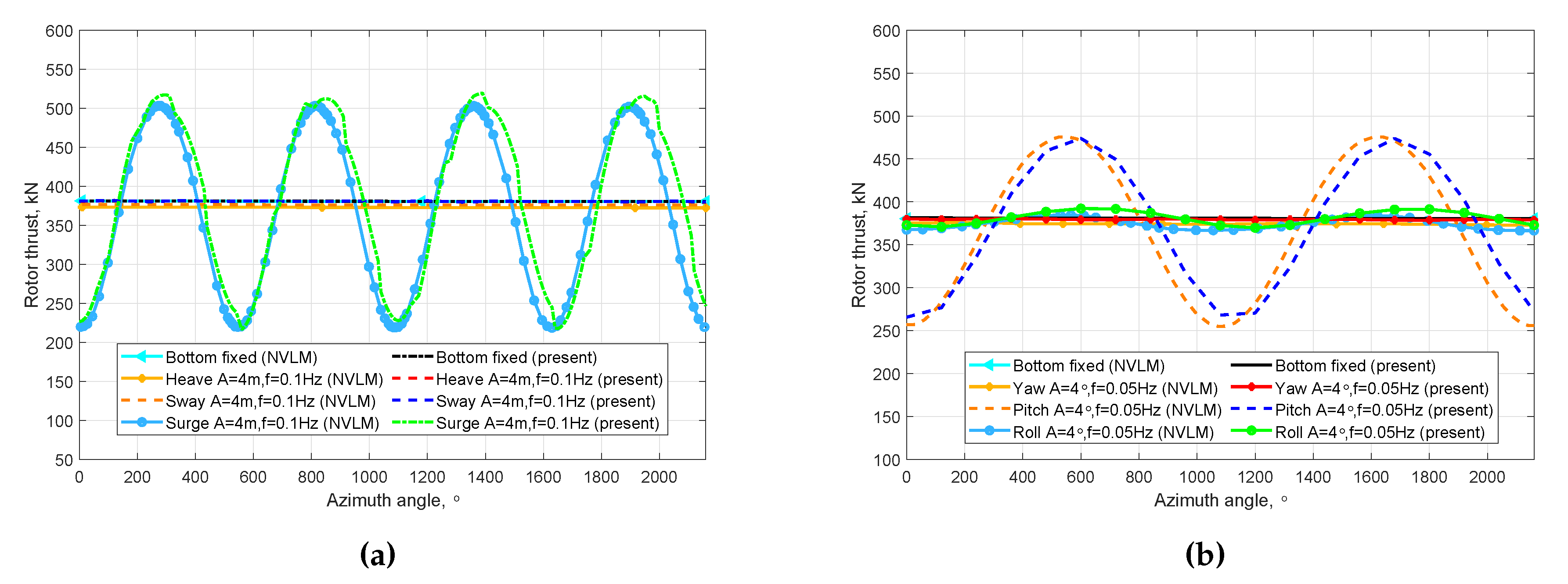
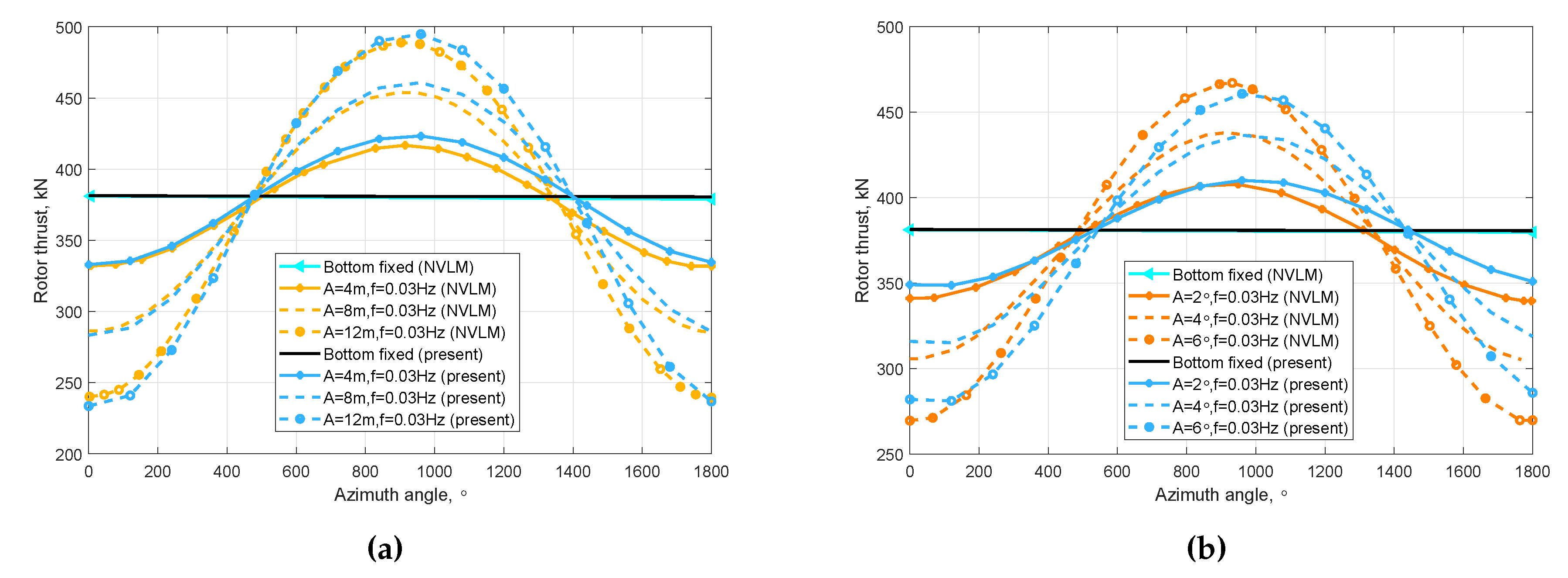
5.2. Floating Wind Turbine under Single-DoF Motion

Since the results from the present vortex ring method are shown to be reliable for a bottom-mounted wind turbine, the method is applied to a floating offshore wind turbine with a platform motion prescribed in one degree of freedom (DoF).

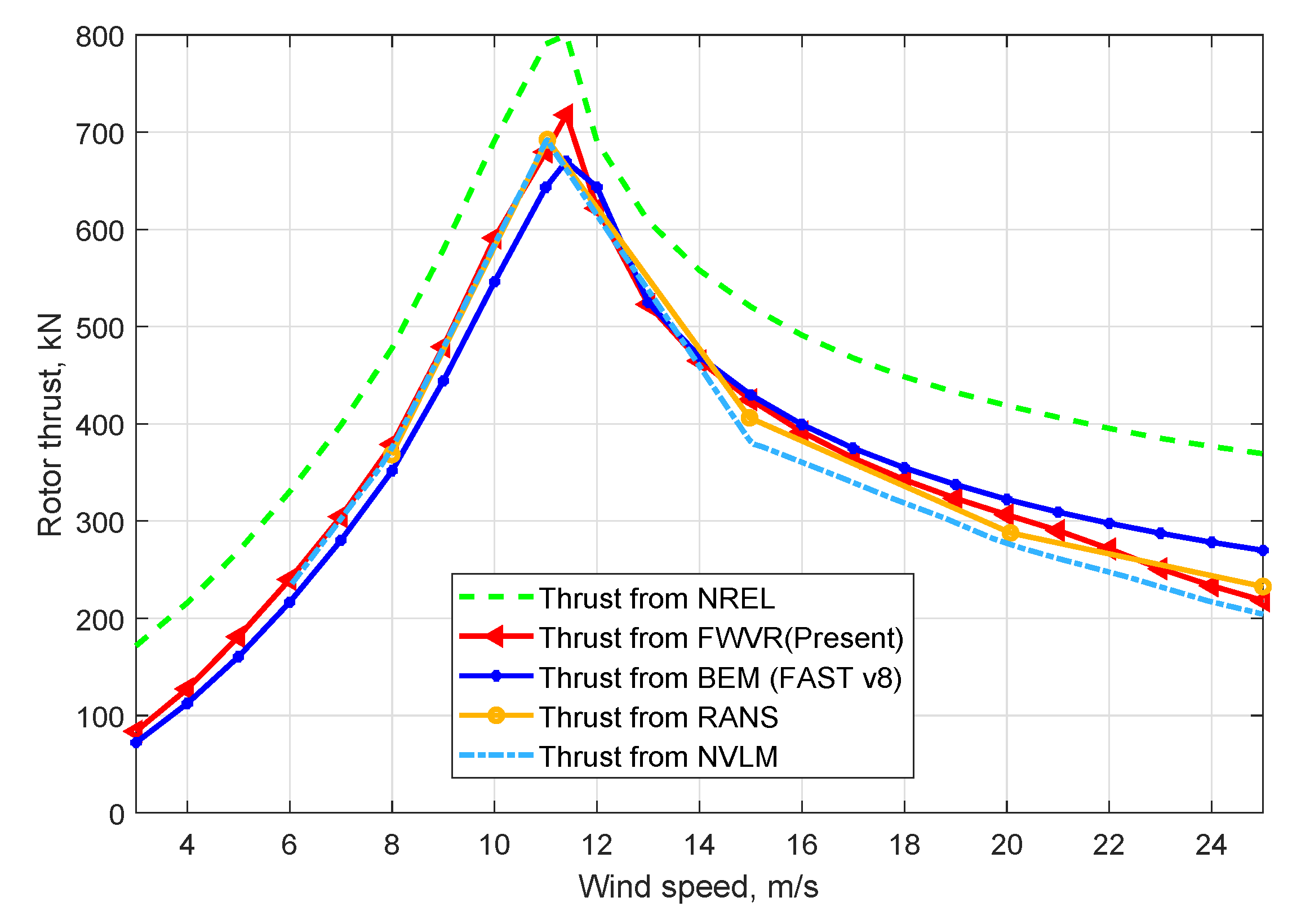
5.2.1. Thrusts Comparison with Lee

The thrusts are calculated with a wind speed of 8 m/s and a rotor speed of 9.16 rpm. The platform motions are defined as a sine function in Equation (56) with amplitude (A) and frequency (f) given in Table 2.
X ( t ) = A 1 sin ( 2 π f 1 t ) .
Figure 8 shows the results of thrusts with translational (surge, sway, and heave, in Figure 8a) and rotational (yaw, pitch, and roll, in Figure 8b) platform motions. The thrust for a fixed rotor is also provided for comparison. For a moving rotor, the thrust forces obtained from both methods have similar amplitude and frequency, which are both consistent with the thrusts shown in Figure 6. Figure 8 shows that the thrust under translational platform motions is most sensitive to surge, and the thrust under rotational platform motions is most sensitive to pitch, for the reason that these motions are in the wind direction, which can significantly influence the relative wind speed normal to the rotor disc. When the rotor has a leeward speed, the relative wind speeds are reduced on the blades and the angle of attacks are smaller, which leads to a lower thrust load than average. When the rotor has a windward speed, the situation is reverse and the thrust load is larger than average. It is also observed that the heave and sway motions of the same amplitude and frequency theoretically have equivalent influence to the rotor thrust. The heave and sway motions can change the relative tangential wind speed on the airfoils, which either increases or decreases the angle of attack according to the azimuthal angle of the blade, thus increasing or decreasing the thrust. However, this influence is relatively small as the change of tangential wind speed is much smaller than the tangential speed coming from the rotor rotation. Figure 8a shows that, with the present FWVR method, the thrust force under heave and sway motions almost overlap and slightly fluctuate around the thrust value of the bottom-mounted turbine, which is deemed to be reasonable.
The effect of the roll motion on the thrust is similar to that of the heave and sway motions, which mainly influence the relative tangential wind speed and the wake induced velocity on the rotor. The yaw motion can reduce the overall wind area of the rotor, hence reducing the thrust load compared to the bottom-mounted turbine, as obtained for both NVLM and FWVR.
The effect of the surge and pitch motions with different amplitudes are further analyzed and compared with the results of [6] in Figure 9. Figure 9a compares the thrust with surge motions with the amplitude of 4 m, 8 m, 12 m and the frequency of 0.03 Hz, while Figure 9b compares the thrust with pitch motions with the amplitude of 2°, 4°, 6° and the frequency of 0.03 Hz. Since the amplitudes of the platform motions are small and the frequency is relatively low, the thrusts change linearly with platform motions for both surge and pitch.

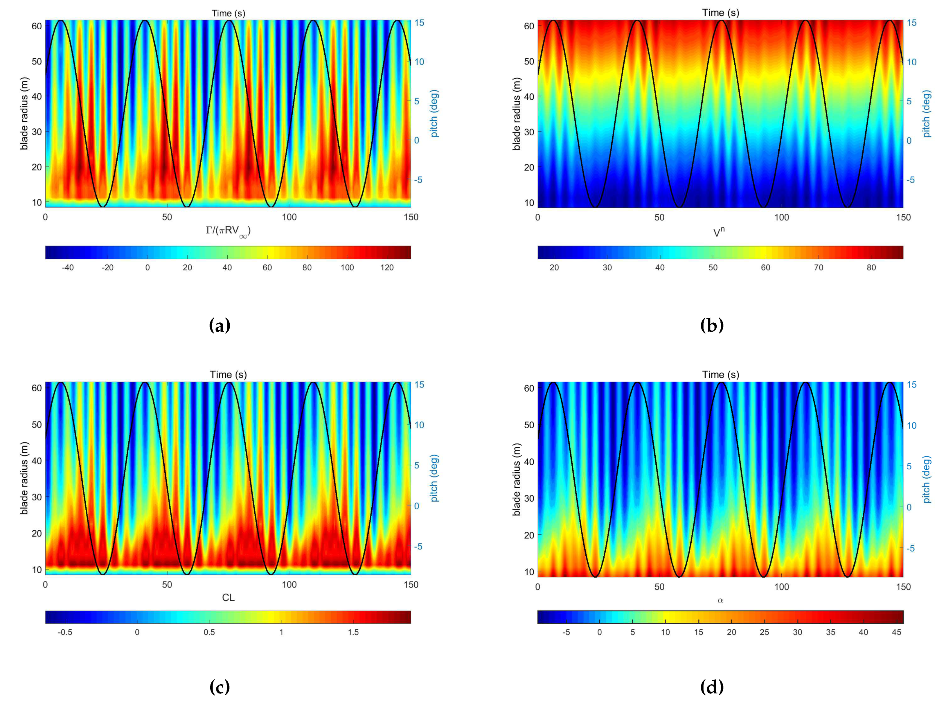
5.2.2. Angle of Attacks Comparison with Sebastian and de Vaal

Additional comparisons are made with the works of Sebastian [5] and de Vaal [14], for different floater types, under the following operating and environmental conditions:
  • below-rated: V = 6.0 m/s, λ = 9.63, H s = 1.83 m, T p = 12.72 s;
  • rated: V = 11.4 m/s, λ = 7.00, H s = 2.54 m, T p = 13.35 s; and
  • above-rated: V = 18.0 m/s, λ = 4.43, H s = 4.09 m, T p = 15.33 s, θ p = 15°
In these works, the platform motions in time domain are synthesised as sinusoidal series at the first two dominant frequencies asthe chord length
X ( t ) = X 0 + A 1 sin ( 2 π f 1 t + ϕ 1 ) + A 2 sin ( 2 π f 2 t + ϕ 2 ) ,
where the mean value X 0 , amplitudes A i , frequencies f i and phase angles ϕ i are given in Table 3.
The mean μ α and standard deviation σ α of the angle of attack α on the outboard 2/3 of the blade are compared in Table 4. The current numerical results are presented in the column entitled “FWVR2, tilt = 0°”, without shaft tilt angle. It is shown that μ α and σ α have the same trend than observed in the literature. In particular, μ α is rather independent of the platform motion, for a given wind speed. The bottom-mounted monopile presents the smallest value of σ α compared with floating support structures at the same wind speed. This can be explained by the fluctuations of the induced velocities caused by turbine-wake interactions in the floating case. The value of σ α increases with the increase of platform motion. In addition, the pitch motions of the platform tend to have more effect on the value of σ α than the surge motions, because the pitch motions generate shear wind velocities on the rotor. The values of μ α are lower than the reference results throughout and the difference are within 1°, which is considered to be acceptable. The column “FWVR2, tilt = 5°” shows the α performance in the design condition of NREL 5 MW with a nonzero tilt angle. It can be seen that the values of μ α are slightly lower than for zero tilt angle, which is mainly because the total wind area is smaller when the rotor is tilted. Moreover, σ α is significantly influenced by the tilt angle in all cases because the latter can generate fluctuating streams especially on the outboard of the blades.

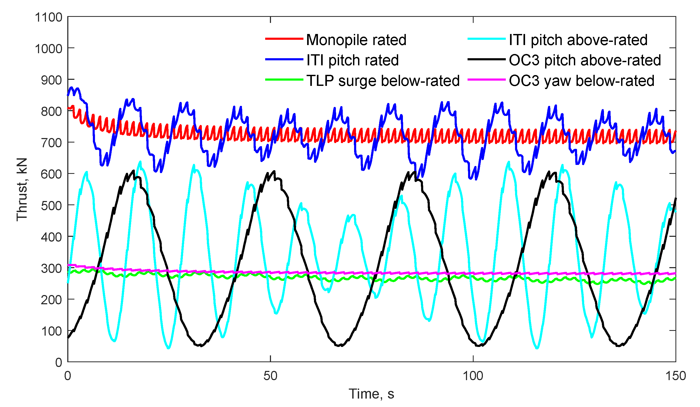
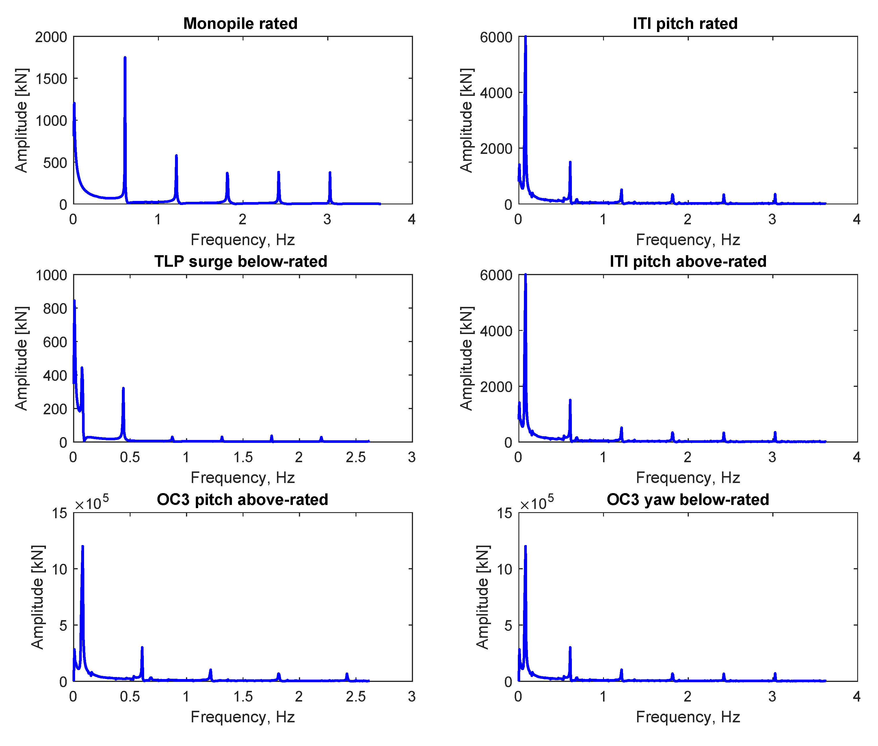
5.2.3. Thrust Analysis in Time Domain and Frequency Domain

The rotor thrust of monopile in rated condition and five floating support structures in below-rated, rated and above-rated conditions are evaluated in time domain (Figure 10) and frequency domain (Figure 11). Figure 10 shows that the thrust fluctuate around their mean values, after an initial transient. The latter is due to the fact that a certain time is needed for the far-wake vortex rings to develop. Thus, initially, only the near wake mostly contributes to the values of induced velocities. After about 50 s, a steady-state is reached and statistics can be taken. Figure 11 highlights the dominant frequencies in the rotor thrust. For a bottom-mounted turbine on a monopile in rated conditions, the first dominant frequency is at about 0.6 Hz, which corresponds to the vortex shedding frequency. Higher frequencies are multiples of the first one. This is due to a periodic process whereby the thrust force reaches a minimum value when the induced velocity reaches a peak value, and vice versa. For the FOWTs, without exception, the frequencies of the platform motions dominate in the frequency of the thrust force. This is because the velocities induced by the platform motions are larger than the induced velocities from the vortex rings.
Finally, we evaluate the blade bounded vortex strength Γ and its relationship with other parameters. As explained above, the value of Γ is obtained by equating the lift forces calculated from the 3D vortex lifting law and that from the blade element theory (see Equation (54)). This leads to:
Γ = c 2 C l ( α ) V n ,
where c is the chord length, C l is the lift coefficient and V n is the normal wind speed. The time evolutions of Γ , V n , C l and α are shown in Figure 12, for the OHS above-rated condition. In each figure, the continuous line represent the platform pitching motion. The non-dimensional Γ / ( π R V ) (Figure 12a) fluctuates with the platform pitch motion. In addition, the high-frequency oscillation with the period of about 4.96 s is due to the rotor tilt angle. On the outboard of the blade, there are negative values of Γ , which is consistent with the negative values of α and C l observed in the same conditions (Figure 12c,d). The normal relative wind speed V n is less influenced by the platform motion and the rotor tilt, its main fluctuations coming from the constant rotation of the rotor.

5.3. Floating Wind Turbine under Multiple-DoF Motion

To conclude this section, three multiple-DOF operating conditions are conducted, combining the properties listed in Table 3, namely:
  • Below-rated: The ITI Energy barge with platform surge, heave, and pitch.
  • Below-rated: The OC3-Hywind spar-buoy with platform pitch and yaw.
  • Above-rated: The OC3-Hywind spar-buoy with platform pitch and yaw.

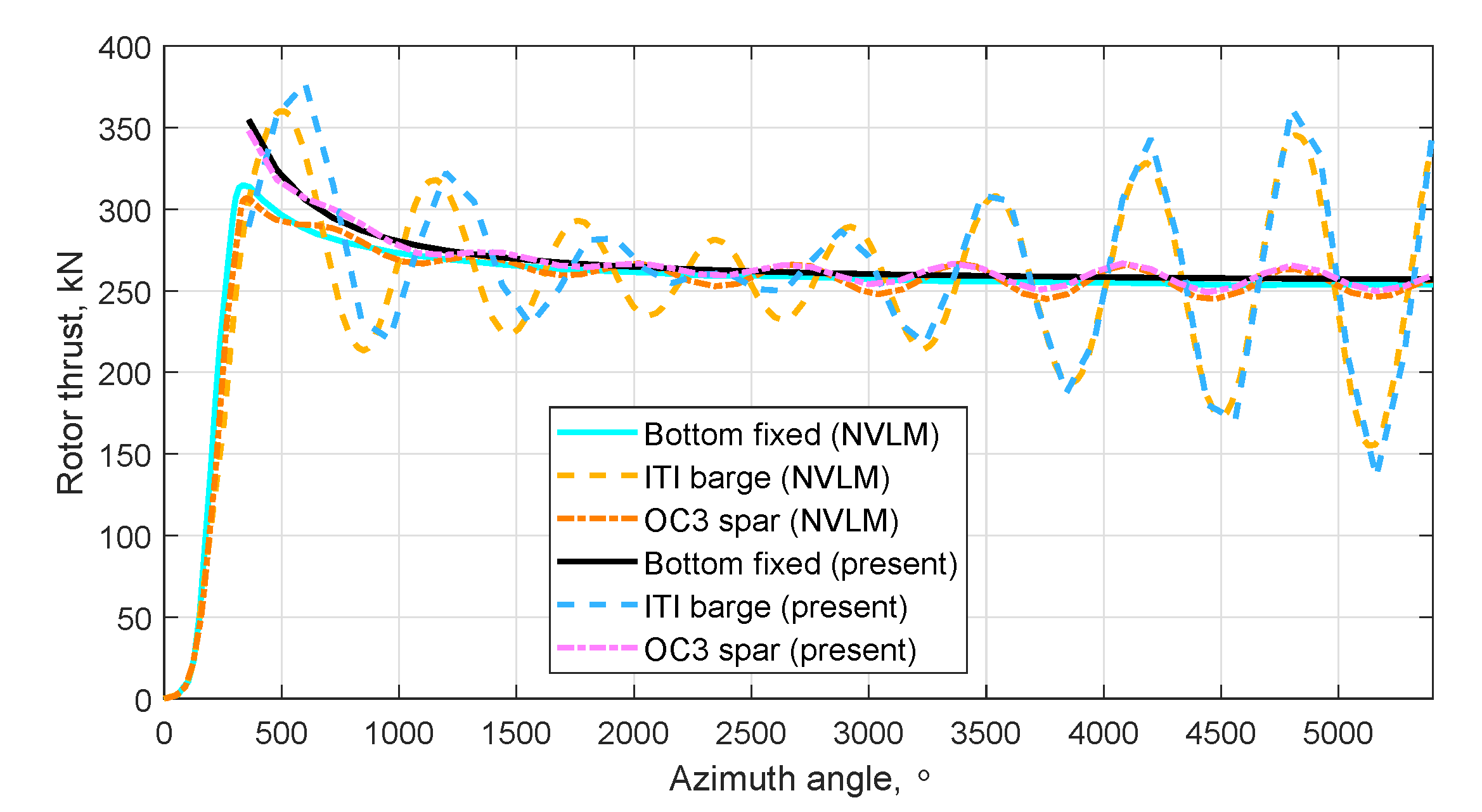
5.3.1. The Multiple-DoF Motion Thrusts Comparison with Lee

The multiple-DoF motion thrusts of ITI and OHS with the below-rated operating conditions as well as the fixed-rotor thrusts are compared with the results of [6] in Figure 13. It should be noted that, the platform motions start at a zero azimuth angle in the FWVR code while they start approximately after one rotation of the rotor in the NVLM code. Therefore, to facilitate the comparison, the thrusts from the present FWVR method is shifted with +360° along the azimuth angle-axis. It is found that the fixed-rotor thrust calculated with the present FWVR method is higher than that calculated with the NVLM method, which is consistent with the previous observation. Besides, the thrust amplitudes and frequencies of the two methods for the ITI and the OHS match well.

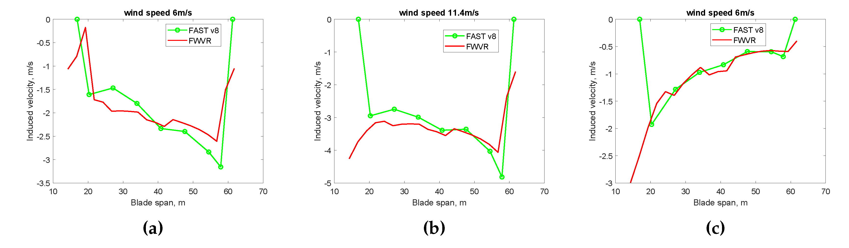
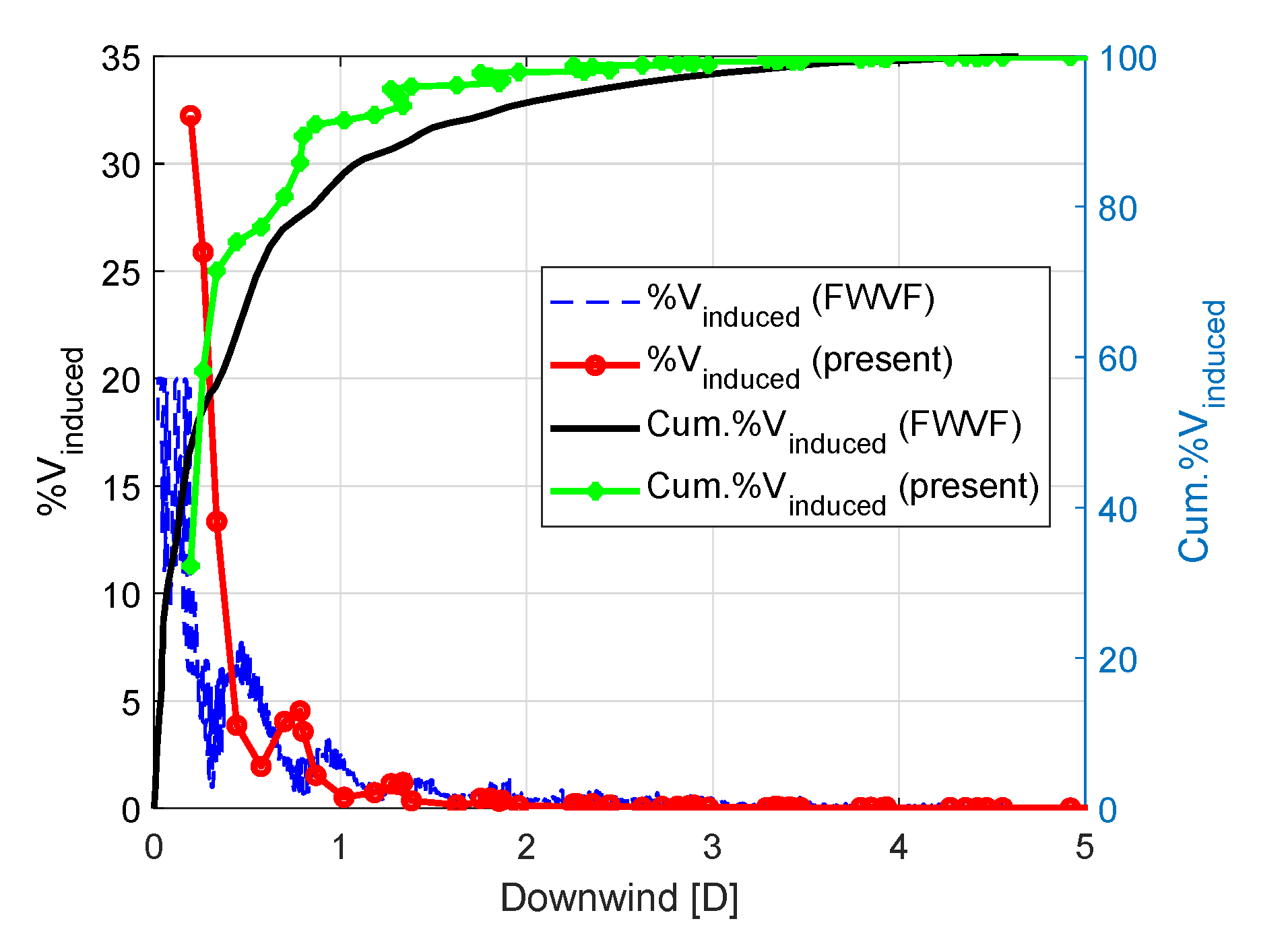
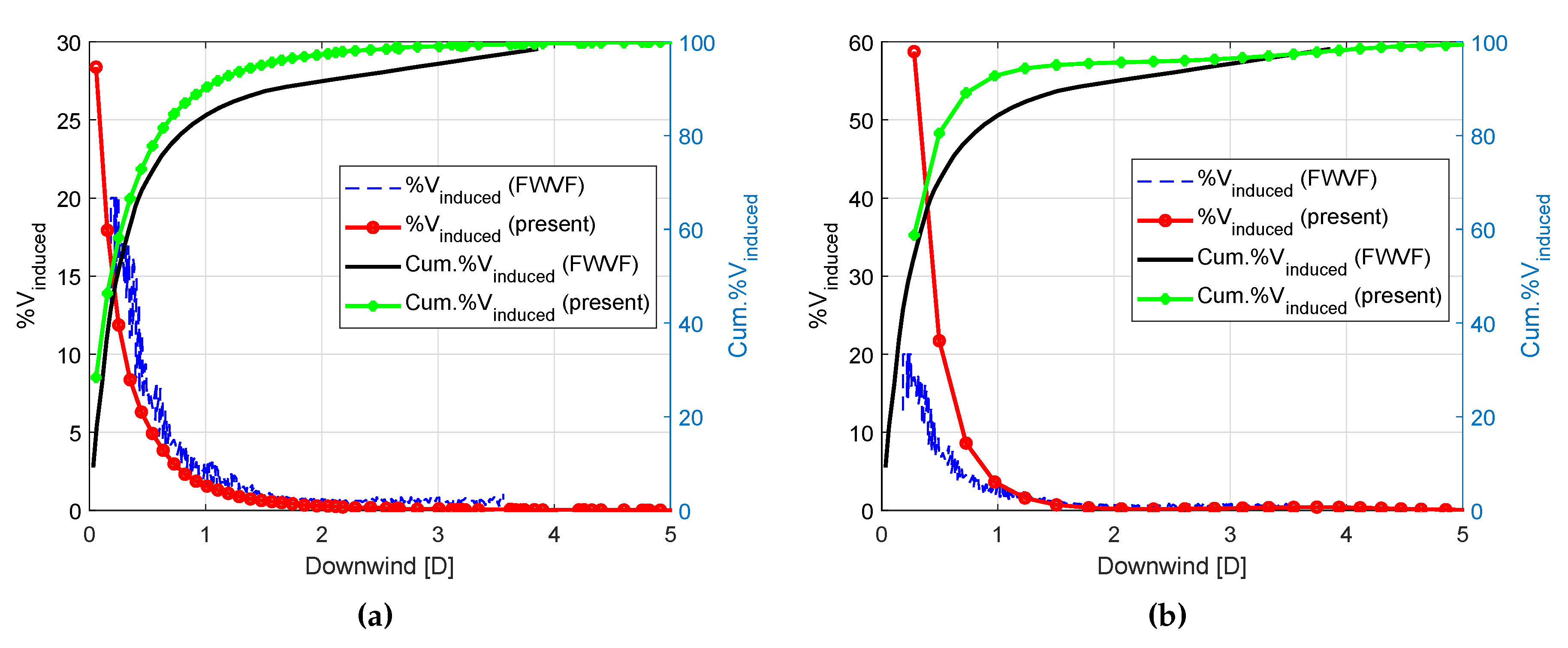
5.3.2. Induced Velocity Comparison with Sebastian

The wake induction at the rotor as a function of the downstream distance of the vortex rings are computed as the percentage of the total induced velocity at the rotor, and compared with [5] in Figure 14 for the ITI and in Figure 15 for the OHS with the NREL 5 MW wind turbine. The blue dashed lines represent the contribution of the induced velocities from each section along the wake as obtained with the FWVF method, while the red lines are the results of the present FWVR method. The red circles on the line highlight the position of the vortex rings. The black lines and the green dotted lines represent the accumulated percentage of the induced velocities along the wake from the FWVF method and FWVR method, respectively. The induced velocity data output from the present FWVR method was captured at the operating time of 150 s, when a stable condition was reached by the wind turbine. Since the convection of the vortex rings downstream is a dynamic process, the induced velocity captured at different time steps can be slightly different.
In general, the induced velocities are comparable between the two methods. As shown in Figure 14, the accumulated percentage of the induced velocity at distances 1D and 2D behind the rotor differ only by 2%, and this difference decreases to maximum 1.0% as the distance behind the rotor increases. Furthermore, the induced velocities from each section along the wake show similar trend with both methods, the big fluctuations being mainly influenced by the platform motions, particularly from the pitch. For the OHS below-rated condition (Figure 15a), a similar discrepancy is observed between the models, with differences of 2.4% and 2.1% at distances of 1D and 2D behind the rotor and 0.6% further downstream. In addition, the influence of the pitch and yaw platform motions on the induced velocity is relatively small. Above rated power (Figure 15b), slightly larger discrepancies are observed, with differences of 9.8% and 4.8% at distances of 1D and 2D behind the rotor and less than 1% further downstream. Additionally, the present FWVR method predicts significantly larger contribution of the induced velocity from the vortex rings within the 1D distance downstream. This is mainly because the vortex rings convect faster with the increase in wind speed, and the density of rings is sparser at higher wind speed. Because the induced velocity is very sensitive to the distance between the control points and the vortex ring (see Equation (21)) the contribution from the front rings is much more significant than that of the rings further away from the rotor. The small differences in the results can be explained from the differences in wake induction of these two methods. The first difference is that the induced velocities of the wake from the FWVF method are output for each vortex segment in the wake, while the induced velocities from the present FWVR method are output for each vortex ring. As explained in Section 4, there are fewer vortex rings than vortex segments in the wake, thus the induced velocities of the wake from the FWVF method are relatively constant compared to those from the FWVR method. The second difference is that, due to the different modeling properties, the induced velocities from the FWVF method start from a position very close to the rotor, while the induced velocities from the present FWVR method start from the position of the first vortex ring, and the induced velocity at the rotor from the near wake model is not accounted here.

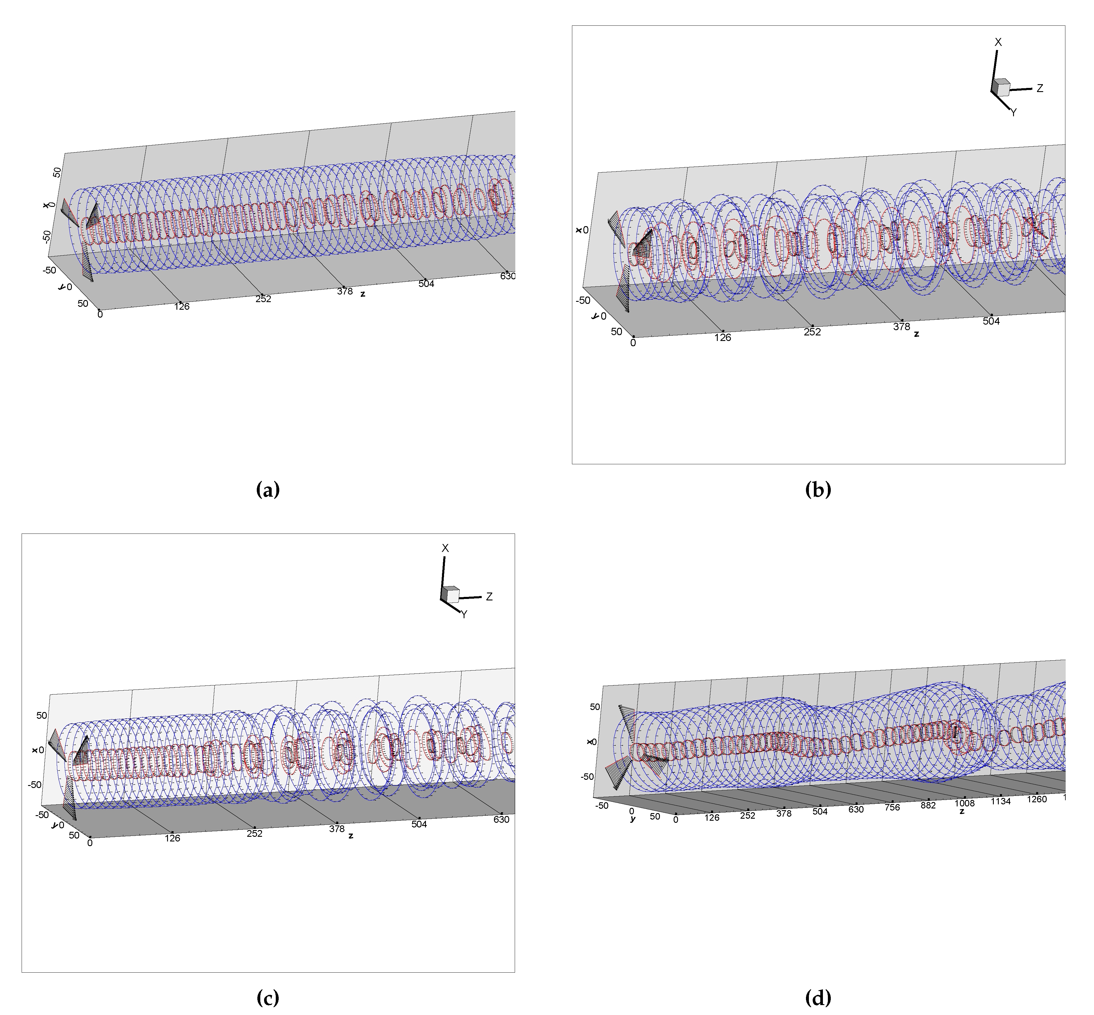
5.3.3. Wake structure discussion

The wake structures of the bottom-fixed wind turbine with the specified below-rated operating condition as well as the FOWTs with the three multiple-DoF platform motions at 150 s of the operating time are shown in Figure 16. The inner and outer rings are distinguished with red and blue colors, respectively, with the vectors indicating the directions where the control points are moving in the next time step. The wake structures of the below-rated operating conditions, as shown in Figure 16a–c, are found to be more compact than the above-rated operating conditions, as shown in Figure 16d, which is due to the different convecting speeds of the vortex rings in the wake in different free stream environments. The wake structure of the bottom-fixed wind turbine has homogeneous vortex ring radii since its blade bound vortex strengths are homogeneous. By contrast, the wake structures of the FOWTs have significant fluctuations because both the blade bound vortex strengths and the rotor position change with time, thus affecting the roll-up process of the wake model. Additionally, the vortex rings in the wake with uneven radii and vortex strengths interacting with each other can cause some fluctuations downstream in the wake, especially below-rated conditions for which the downstream vortex rings are relatively close to one another, which can be seen clearly in Figure 16b,c.

6. Conclusions

In this paper, a simplified free wake vortex ring method for horizontal-axis wind turbine is modified and assessed. A new trailed vortex model with finite length vortex lines is proposed. The NREL 5 MW wind turbine was used to validate the code extensively for the cases of monopile wind turbine, single-Dof platform motions and mutiple-Dof platform motions, respectively, where the thrusts, angle of attacks, and induced velocities are found to have good agreement with the literature. To conclude, the modified free wake vortex ring method proposed here is considered to be effective when solving the aerodynamic load around horizontal-axis wind turbines, on both fixed and floating support structures.

Author Contributions

Conceptualization, J.D. and A.V.; methodology, J.D.; software, J.D.; validation, J.D., A.V. and C.S.F.; formal analysis, J.D.; investigation, J.D.; resources, Z.L.; data curation, J.D.; writing—original draft preparation, J.D.; writing—review and editing, A.V. and C.S.F.; visualization, J.D. and Z.L.; supervision, A.V. and G.v.B.; project administration, A.V.; and funding acquisition, J.D., A.V. and G.v.B.

Funding

This research was funded by China Scholarship Council (CSC).

Acknowledgments

Dong would like to acknowledge support from China Scholarship Council (CSC). Viré acknowledges support from the Rijksdienst voor Ondernemend Nederland (RVO) through the TSE Hernieuwbare Energie funding scheme (ABIBA project). Many thanks are also extended to Jacobus B. de Vaal of the Institute for Energy Technology in Norway for his generous assistance in this work. Special thanks are also given to Jason Jonkman of NREL for his valuable guidance of using FAST.

Conflicts of Interest

The authors declare no conflict of interest. The funders had no role in the design of the study; in the collection, analyses, or interpretation of data; in the writing of the manuscript, or in the decision to publish the results.

Abbreviations

The following abbreviations are used in this manuscript:
FOWTFloating Offshore Wind Turbines
BEMBlade Element Momentum Theory
CFDComputational Fluid Dynamics
NRELNational Renewable Energy Laboratory
FWVFFree Wake Vortex Filament Method
NVLMNonlinear Vortex Lattice Method
FWVRFree Wake Vortex Ring Method
CO3Code Comparison Collaboration
OHSOC3-Hywind Spar-Buoy
TLPTension Leg Platform
RANSReynolds-averaged Navier–Stokes Method
AFWRVActuator Disc with Free Wake Vortex Ring Model

References

  1. Sebastian, T.; Lackner, M. Characterization of the unsteady aerodynamics of offshore floating wind turbines. Wind Energy 2013, 16, 339–352. [Google Scholar] [CrossRef]
  2. Emmanuel, B. Wind Turbine Aerodynamics and Vorticity-Based Methods, Fundamentals and Recent Applications; Springer: Berlin/Heidelberg, Germany, 2017. [Google Scholar]
  3. Bhagwat, M.; Leishman, J. Transient Rotor Inflow Using a Time-Accurate Free-Vortex Wake Model. In Proceedings of the AIAA, Aerospace Sciences Meeting and Exhibit, Reno, NV, USA, 8–11 January 2001. [Google Scholar] [CrossRef]
  4. Gohard, J.C. Free Wake Analysis of Wind Turbine Aerodynamics; Technical Report; MIT: Cambridge, MA, USA, 1978. [Google Scholar]
  5. Sebastian, T.; Lackner, M. Analysis of the Induction and Wake Evolution of an Offshore Floating Wind Turbine. Energies 2012, 5, 968–1000. [Google Scholar] [CrossRef] [Green Version]
  6. Lee, H.; Lee, D.J. Effects of platform motions on aerodynamic performance and unsteady wake evolution of a floating offshore wind turbine. Renew. Energy 2019, 143, 9–23. [Google Scholar] [CrossRef]
  7. Newman, S. The Induced Velocity of a Vortex Ring Filament; AFM Technical Reports 11/03; University of Southampton, School of Engineering Sciences: Southampton, UK, 2011. [Google Scholar]
  8. Yoon, S.; Heister, S. Analytical formulas for the velocity field induced by an infinitely thin vortex ring. Int. J. Numer. Methods Fluids 2004, 44, 665–672. [Google Scholar] [CrossRef]
  9. Øye, S. A simple vortex model. In Proceedings of the Third IEA Symposium on the Aerodynamics of Wind Turbines, ETSU, Harwell, UK, 16–17 November 1989. [Google Scholar]
  10. De Vaal, J.; Hansen, M.; Moan, T. Validation of a vortex ring wake model suited for aeroelastic simulations of floating wind turbines. J. Phys. Conf. Ser. 2014, 555, 012025. [Google Scholar] [CrossRef]
  11. Yu, W.; Ferreira, C.S.; van Kuik, G.; Baldacchino, D. Verifying the Blade Element Momentum Method in unsteady, radially varied, axisymmetric loading using a vortex ring model. Wind Energy 2017, 20, 269–288. [Google Scholar] [CrossRef]
  12. Miller, R. Simplified Free Wake Analysis for Rotors; Technical Report; Aeronautical Research Inst.: Stockholm, Sweden; National Aeronautics and Space Administration: Washington, DC, USA, 1982.
  13. Afjeh, A. Wake Effects on the Aerodynamic Performance of Horizontal Axis Wind Turbines; NASA STI/Recon Technical Report N; NASA STI: Hampton, VA, USA, 1984.
  14. De Vaal, J.; Hansen, M.; Moan, T. Influence of Rigid Body Motions on Rotor Induced Velocities and Aerodynamic Loads of a Floating Horizontal Axis Wind Turbine. In Proceedings of the ASME, International Conference on Offshore Mechanics and Arctic Engineering, San Francisco, CA, USA, 8–13 June 2014. [Google Scholar] [CrossRef]
  15. De Vaal, J. Aerodynamic Modelling of Floating Wind Turbines. Ph.D. Thesis, NTNU, Trondheim, Norway, 2015. [Google Scholar]
  16. Sørensen, N.; Johansen, J. UPWIND, Aerodynamics and Aero-elasticity Rotor Aerodynamics in Atmospheric Shear Flow; Invited Presentation. Published at the Web.; European Wind Energy Conference & Exhibition, EWEC: Copenhagen, Denmark, 2007. [Google Scholar]
  17. Leonard, A. Computing Three-Dimensional Incompressible Flows with Vortex Elements. Annu. Rev. Fluid Mech. 1985, 17, 523–559. [Google Scholar] [CrossRef]
  18. Van Hoydonck, W.; Gerritsma, M.; van Tooren, M. On Core and Curvature Corrections used in Straight-Line Vortex Filament Methods. J. Am. Helicopter Soc. arXiv 2012, arXiv:1204.2699. [Google Scholar]
  19. Betz, A. Behavior of Vortex Systems; Technical Reports NACA-TM-713; National Advisory Committee for Aeronautics: Washington, DC, USA, 1993.
  20. Phillips, W.F.; Snyder, D. Modern Adaptation of Prandtl’s Classic Lifting-Line Theory. J. Aircr. 2000, 34, 622–670. [Google Scholar] [CrossRef]
  21. Van Garrel, A. Requirements for a Wind Turbine Aerodynamics Simulations Module—Version 1; ECN-C-01-099; Energy Research Centre of The Netherlands (ECN): Petten, The Netherlands, 2001. [Google Scholar]
  22. Jonkman, J.; Butterfield, S.; Musial, W.; Scott, G. Definition of a 5-MW Reference Wind Turbine for Offshore System Development; Technical Report; National Renewable Energy Laboratory: Golden, CO, USA, 2009. [Google Scholar]
Figure 1. Coordinate system associated with a vortex ring.
Energies 12 03900 g001
Figure 2. The blade bound vortex model.
Energies 12 03900 g002
Figure 3. The trailed vortex models: infinite length (a); and finite length (b).
Energies 12 03900 g003
Figure 4. Schematic representation of a four vortex rings (b) shed by the far wake model (a).
Energies 12 03900 g004
Figure 5. Forces acting on a blade element.
Energies 12 03900 g005
Figure 6. The thrust of monopile NREL 5 MW wind turbine as a function of the wind speed.
Energies 12 03900 g006
Figure 7. The axial induced velocities at wind speeds 6 m/s (a), 11.4 m/s (b) and 18 m/s (c).
Energies 12 03900 g007
Figure 8. Thrust with: (a) translational motions (A = 4 m, f = 0.1 Hz); and (b) rotational motions (A = 4°, f = 0.05 Hz).
Energies 12 03900 g008
Figure 9. Thrust with: (a) surge (A = 4 m, 8 m, 12 m, f = 0.03 Hz); and (b) pitch (A = 2°, 4°, 6°, f = 0.03 Hz).
Energies 12 03900 g009
Figure 10. Time evolution of the thrust force on the rotor for different turbine configurations.
Energies 12 03900 g010
Figure 11. Frequency content of the thrust force on the rotor for different turbine configurations.
Energies 12 03900 g011
Figure 12. Time evolution of: (a) Γ / ( π R V ) ; (b) V n ; (c) C l ; and (d) α for the OHS above-rated condition.
Energies 12 03900 g012
Figure 13. Variation in the thrust of 5 MW NREL wind turbine in multiple-DoF motions.
Energies 12 03900 g013
Figure 14. Wake induced velocity at the rotor for the NREL 5 MW turbine + ITI with surge, heave, and pitch for below-rated conditions.
Energies 12 03900 g014
Figure 15. Wake induced velocity at the rotor for the NREL 5 MW turbine + OHS under pitch and yaw: (a) below-rated; and (b) above-rated.
Energies 12 03900 g015
Figure 16. Wake structures of the NREL 5 MW turbine: (a) bottom fixed below-rated; (b) ITI barge below-rated; (c) OHS below-rated; and (d) OHS above-rated.
Energies 12 03900 g016
Table 1. Computational time and function of different models.
MethodComputational TimeModeling Capability
BEM C b N θ N Ω Rotor aerodynamics without wake
AFWVR 1 3 C a N b 2 N θ 2 N Ω 3 Rotor aerodynamics, uncoupled wake aerodynamics
FWVR 1 3 C r N b 2 N θ 2 N Ω 3 + C Γ N θ N Ω Coupled rotor aerodynamics and wake aerodynamics
FWVF 1 3 C f N b 2 N θ 3 N Ω 3 + C Γ N θ N Ω Coupled rotor aerodynamics and wake aerodynamics
NVLM 1 3 C m N b 2 N θ 3 N Ω 3 + C Γ N θ N Ω Coupled rotor aerodynamics and wake aerodynamics
Table 2. Amplitude and frequency of prescribed single-DoF motions [6].
MotionAmplitude A [m or °]Frequency f [Hz]
Translation (surge, sway, heave)40.1
Rotation (roll, pitch, yaw)40.05
surge4,8,120.03
pitch2,4,60.03
Table 3. Parameters of platform motions [5] for the NREL 5 MW turbine with different floater types.
Oper.Platf.Mode X 0 A 1 f 1 ϕ 1 A 2 f 2 ϕ 2
[m]/[°][m]/[°][Hz][rad][m]/[°][m]/[°][rad]
1ITIsurge13.6020.7250.007−1.163−0.4420.0782.609
1ITIheave−0.1300.3180.0781.3030.2540.1082.702
1ITIpitch0.5911.4750.078−0.0661.6300.0831.816
1OHSpitch1.580−0.0840.0661.930−0.1160.0773.113
1OHSyaw−0.0210.0910.1081.983−0.0360.1203.429
1TLPsurge1.2060.4360.016−0.831−0.2220.0773.018
2ITIpitch1.722−0.6370.065−0.3811.6770.0771.835
3ITIpitch0.9391.5180.0662.1322.9790.0786.863
3OHSpitch3.32411.9610.0290.4200.0000.0000.000
3OHSyaw−0.2222.0000.029−0.3593.1850.0583.385
Table 4. Mean and standard deviation of α at the outboard 2/3 part of the blade.
OperationPlatformModeWInDS [5]FWVR1 [14]FWVR2, tilt = 0°FWVR2, tilt = 5°
μ α [°] σ α [°] μ α [°] σ α [°] μ α [°] σ α [°] μ α [°] σ α [°]
1Monopile3.950.233.860.483.820.153.713.23
1ITIsurge3.950.403.870.533.780.233.643.23
1ITIpitch3.992.213.901.53.891.923.843.85
1OHSpitch3.940.323.840.493.660.253.843.21
1TLPsurge3.950.273.860.493.640.233.703.23
2Monopile6.760.376.660.695.840.355.763.35
2ITIpitch6.781.676.671.305.821.095.733.47
3Monopile−0.100.80−0.312.24−0.590.05−0.612.91
3ITIpitch−0.082.26−0.282.88−0.591.87−0.613.39
3OHSpitch−0.453.59−0.523.09−0.832.40−0.853.57

