Accurate Parameter Estimation of a Hydro-Turbine Regulation System Using Adaptive Fuzzy Particle Swarm Optimization

Abstract

Parameter estimation is an important part in the modeling of a hydro-turbine regulation system (HTRS), and the results determine the final accuracy of a model. A hydro-turbine is normally a non-minimum phase system with strong nonlinearity and time-varying parameters. For the parameter estimation of such a nonlinear system, heuristic algorithms are more advantageous than traditional mathematical methods. However, most heuristics based algorithms and their improved versions are not adaptive, which means that the appropriate parameters of an algorithm need to be manually found to keep the algorithm performing optimally in solving similar problems. To solve this problem, an adaptive fuzzy particle swarm optimization (AFPSO) algorithm that dynamically tunes the parameters according to model error is proposed and applied to the parameter estimation of the HTRS. The simulation studies show that the proposed AFPSO contributes to lower model error and higher identification accuracy compared with some traditional heuristic algorithms. Importantly, it avoids a possible deterioration in the performance of an algorithm caused by inappropriate parameter selection.

1. Introduction

System identification is an important branch of modern control theory. The principle is to find a mathematical model that best fits the dynamic characteristics of a real system in a specified model set according to the input and output data of the system [1]. When the structure of a model is known but its parameters are unknown, system identification can be simplified to a parameter estimation problem. Hydro-turbine regulation system (HTRS) is a common energy conversion system in the field of renewable energy. It consists of governor, turbine, water diversion system, generator and load [2,3]. HTRS is a complex nonlinear system of hydraulic-mechanical-electrical coupling. The basic structure of its mathematical model has been theoretically studied and experimentally verified [4,5,6,7]. Therefore, the key to establishing its precise mathematical model is to design an effective parameter estimation method.

The heuristic optimization algorithm is a mature and widely used model parameter estimation method in engineering [8,9]. Compared with the traditional deterministic optimization methods, it is not limited by the complexity of models, and can efficiently solve high-dimensional single-objective or multi-objective optimization problems. The core idea of the method is to use a certain evolutionary strategy and a predefined objective function to estimate a set of optimal parameters to minimize the error between the predicted and ideal values of the output of the system studied. The heuristic algorithm, known as particle swarm optimization (PSO), was developed a number of years back and has been successfully used to solve various practical problems faced by renewable energy systems, such as parameter estimation, optimization control and energy management [10,11,12,13,14,15,16]. In order to improve the convergence speed of traditional algorithms and reduce the risk of premature convergence, the advantages of PSO and genetic algorithms (GA) have been combined, and an optimal energy demand estimation model based on PSO-GA is proposed in the literature [17]. An improved gravitational search algorithm (GSA) with the update mechanism of particle position of PSO and a weighted fitness function is proposed in [18] to realize accurate identification of HTRS. To further improve the convergence speed and accuracy of GSA, chaotic local search and elastic ball theory are added in the iterative process of the algorithm in [19] to obtain an ideal identification result.

However, similar to most heuristic algorithms, basic PSO may also suffer from the problems of premature convergence and trapping into local optima [20,21]. At the same time, the parameter selection of the algorithm depends largely on experiments and experience, and unreasonable parameters will greatly reduce the performance of the algorithm [22]. The improvement of PSO mainly focuses on strengthening its ability to jump out of local optimum in solving multi-modal complex optimization problems.

There are two main categories of improvement strategies. The first category is the improvement of the algorithm itself, such as the extension of the scope of algorithm [23,24], the optimization of algorithm parameters and neighborhood structure [25,26,27], and the improvement of the evolutionary strategy [28]. Authors of [24] proposed a binary discrete PSO for solving discrete space optimization problems, but local convergence and computational redundancy are the main problems faced by the algorithm. The introduction of dynamic niche technology into PSO in [29] significantly improved the search efficiency and accuracy of the algorithm. The second category is the fusion of PSO with other intelligent algorithms or operators, such as simulated annealing [30], mutation operator [31], and local search strategy [19]. Cooperative particle swarm optimization is successfully proposed in [32,33,34] and quantum particle swarm optimization is proposed in [35,36,37]. It should be noted that although these improved algorithms have their own advantages, new structures and parameters are inevitably introduced, which increases the complexity of the algorithms and limits their application.

As pointed out in [38,39], the automatic design and selection of evolutionary algorithms is an effective way to improve the performance of the algorithm. It is also a research hotspot and development trend in this field. To avoid parameter selection and overcome the premature convergence problem, an adaptive fuzzy particle swarm optimization (AFPSO) based on a fuzzy inference system, variable neighborhood search strategy and hybrid evolution is proposed in this paper and applied to the parameter estimation of nonlinear HTRS. The main contributions of this work are: (1) Provide an adaptive parameter tuning strategy to overcome the difficulty in algorithm parameter selection; (2) Adopt a comprehensive objective function that considers output error and correlation coefficient to make the parameter estimation more reliable; (3) In order to reflect the dynamic characteristics of a real system, a general simulation model of nonlinear HTRS is established. Compared to linear systems, the parameter estimation of nonlinear systems is more difficult because activated nonlinear parts are not sensitive to signal changes. For example, when a saturated nonlinear part is activated, the output of the system remains constant regardless of how the input changes. Therefore, it is importantly meaningful to study the parameter estimation of nonlinear systems.

The rest of this paper is organized as follows. In Section 2, the modeling method of each subsystem of HTRS is introduced, and a nonlinear simulation model is built. In Section 3, the principles of the basic PSO are briefly described and three specific improvements are proposed. The definition of objective function and the implementation of parameter estimation strategy are stated in detail in the next section. Performance of the new algorithm is evaluated in Section 5 by comparative studies on the parameter estimation of HTRS under two operating conditions, and conclusions are drawn in the final section.

2. Mathematical Model of HTRS

As shown in Figure 1, HTRS is a complex nonlinear system consisting of controller, servo-system, hydro-turbine and water diversion system, generator and load. There is a hydraulic-mechanical-electrical coupling effect in the system, in which the nonlinear factors of the governor have an important influence on the dynamic characteristics of the system. For example, factors such as the dead zone, saturation, and delay may change the behavior of the servomotor. The research object in this paper is a nonlinear HTRS including the nonlinear factors of a servo-system. The mathematical model of each part of the system is presented below.

1. Controller

At present, governors with a PID control law are widely used in hydropower plants. Although many advanced control strategies or intelligent controllers for HTRS have been proposed, these methods are still in the simulation stage and have not been verified. The general mathematical expression of a parallel PID governor is shown in Equations (1) and (2).

$$\frac{u}{e}=K_P+\frac{K_I}{s}+\frac{K_{D}s}{T_{1v}s+1}$$

(1)

$$e=\left(x_c-x\right)+b_p\left(y_c-y\right)$$

(2)

where $x_c$ and $x$ are the given and measured values of generator speed respectively, while $y_c$ and $y$ are the given and measured values of guide vane opening (GVO) respectively; $e$ and $u$ are the error and output of the controller respectively; $K_P$, $K_I$ and $K_D$ are the proportional, integral and differential gains of the controller respectively; $T_{1v}$ is the differential time constant; $s$ is the Laplace variable; and $b_p$ is the permanent speed drop.

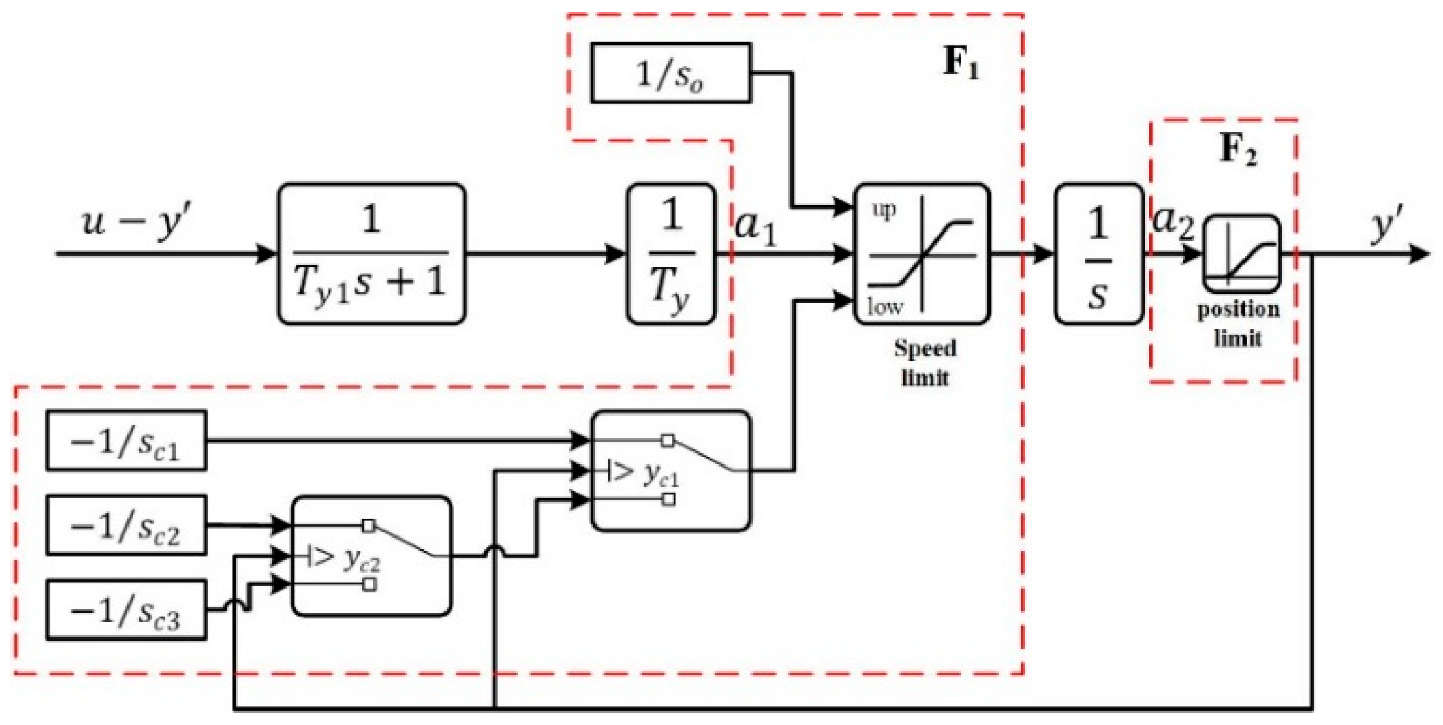
2. Servo-system

The simplified model commonly used in the servo-system is derived from the equation of motion of the servomotor, Equation (3). To get closer to the real situation, the nonlinear dynamic behavior in the servo-system, including saturation, speed limit and delay, are considered in the parameter estimation of the HTRS, which is shown in Equations (3)–(6) or Figure 2 and Figure 3.

$$\frac{y^{\prime }}{u-y^{\prime }}=F_2\left(F_1\left(\frac{1}{T_{y1}s+1}·\frac{1}{T_y}\right)\frac{1}{s}\right)$$

(3)

$$y=y^{\prime }{e}^{-T_{d}s}$$

(4)

$$F_1\left(a_1\right)=\{\begin{array}{ll}min\left\{1/s_o,a_1\right\},& a_1\ge 0\\ max\left\{-1/s_{c1},a_1\right\},& a_1<0 \mathrm{and} y^{\prime }>y_{c1}\\ max\left\{-1/s_{c2},a_1\right\},& a_1<0 \mathrm{and} y_{c2}<y^{\prime }\le y_{c1}\\ max\left\{-1/s_{c3},a_1\right\},& a_1<0 \mathrm{and} y^{\prime }\le y_{c2}\end{array}$$

(5)

$$F_2\left(a_2\right)=min\left\{y_{max},max\left\{y_{min},a_2\right\}\right\}$$

(6)

where $T_y$ and $T_{y1}$ are defined as the response time constant of servomotor and that of auxiliary servomotor, respectively; Both $y$ and $y^{\prime }$ are GVO, and the difference is that the former is obtained by applying a certain delay $T_d$ to the latter; $F_1$ is a speed limit function with the input variable $a_1$, including a three-stage closing rule to realize the sequence closing of guide vane, where $s_{c1}$, $s_{c2}$ and $s_{c3}$ are the closing speed limits under different range of GVO, $y_{c1}$, $y_{c2}$ and $y_{c3}$ are the three GVO nodes of the sequence closing, and $s_o$ is the opening speed limit of guide vane. $F_2$ is a position limit function with the input variable $a_2$, and $y_{min}$ and $y_{max}$ are the minimum and maximum of GVO.

3. Water diversion system

The model of water diversion system can be divided into rigid water hammer model and elastic water hammer model. In engineering, an appropriate model is usually selected according to the penstock length of a hydropower station. When the penstock is long enough, the elastic model that considers the elasticity of water and penstock can better reflect the water hammer phenomenon. According to the actual situation of the hydropower station studied, the rigid model, Equation (7), is adopted in this paper:

$$\frac{h}{q}=-T_{w}s$$

(7)

where h and q are the water head and discharge of a hydro-turbine; T_w represents the flow inertia time constant.

4. Hydro-turbine

In the case of small disturbances, a local linear model can be utilized to describe the discharge and torque characteristics of a hydro-turbine, which can be written as:

$$q=e_{qx}x+e_{qy}y+e_{qh}h$$

(8)

$$m_t=e_{x}x+e_{y}y+e_{h}h$$

(9)

where $m_t$ is the torque of a hydro-turbine; $e_{qx}$, $e_{qy}$ and $e_{qh}$ are the transfer coefficients relating to the discharge; and $e_x$, $e_y$ and $e_h$ are the transfer coefficients relating to the torque.

5. Generator

If electrical transients are not considered, a generator can be described by a first-order model derived from the equation of motion of its rotor, namely:

$$\frac{x}{m_t-m_g}=\frac{1}{T_{a}s+e_g}$$

(10)

where $T_a$ is the unit inertia time constant;$e_g$ is the adjusting coefficient of generator; and $m_g$ represents the change of load.

Combining Equations (1) through (10), the overall nonlinear model of the HTRS can be obtained as shown in Figure 3.

3. Improved Particle Swarm Optimization

3.1. Basic PSO

PSO is an optimization algorithm based on swarm intelligence, which is derived from the study of foraging behavior of birds in nature. Based on the observation of the activities of animal groups, the information sharing mechanism among individuals in a group is used to make the movement of the group show a variation from disorder to order and, therefore, complete the search for the optimal target. In the basic PSO, position and velocity are the two basic properties of a particle. At any time, the velocity of the particle is affected by the current velocity, the historical optimal position of the individual, and the historical optimal position of the population. The update rules for velocity and position of particles in basic PSO are shown in Equations (11) and (12).

$$v_i^j\left(t+1\right)=w{v}_i^j\left(t\right)+c_1\left(p_i^j-x_i^j\left(t\right)\right)+c_2\left(g^j-x_i^j\left(t\right)\right)$$

(11)

$$x_i^j\left(t+1\right)=x_i^j\left(t\right)+v_i^j\left(t+1\right)$$

(12)

where $w$ is inertia weight; $c_1$ and $c_2$ are learning factors; $t$ is the number of iterations; $p_i^j$ and $g^j$ are the historical optimal position of the individual and that of the population, respectively; and $v_i^j\left(t\right)$ and $x_i^j\left(t\right)$ represent the velocity and position of the j-th dimension of the i-th particle in the t-th iteration.

As can be seen from the update rules, the flight trajectory of a particle is determined by the following three parts. The first part is the inertia of the particle, reflecting the current velocity. The second part is the self-cognition of the particle, reflecting the distance between the current position and the optimal position experienced by itself. The third part is the social cognition of the particle, reflecting the distance between the current position and the optimal location experienced by the population. This memory-based information sharing mechanism makes the algorithm have a faster convergence speed but easily falls into a local optimum.

3.2. Improvements on PSO

The main disadvantages of the basic PSO can be summarized as parameter settings and algorithm topologies. Firstly, the inertia weight is the crucial control parameter in PSO that affects the search ability and should be adjusted throughout the evolution process, while in basic PSO it is set only before the iteration begins. At the same time, the position and velocity update of each particle partly depends on the global best position provided by the information from all particles. The authors of [40] studied the information transmission and communication in particle swarms based on the biosocial model, finding that individuals in biological society cannot recognize and communicate with all other individuals, and usually are only affected by a small number of individuals around them. Therefore, the algorithm topology should also be flexibly designed to conform to the basic laws of the actual biosocial model. In addition, it is worth noting that mutation is an effective means of getting rid of local extremum, which is lacking in basic PSO. Based on the above analysis, PSO will be modified from the following three aspects.

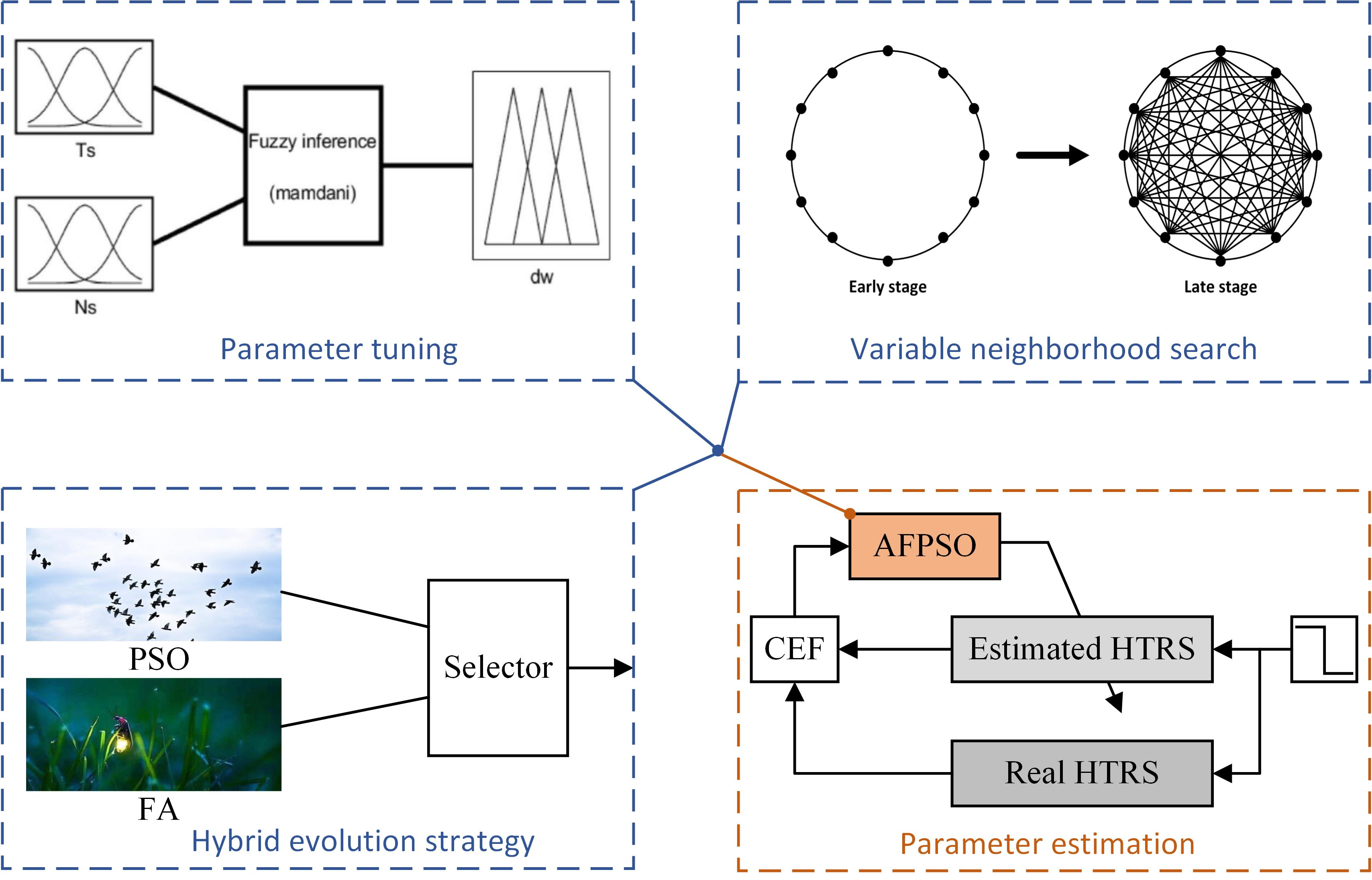
3.2.1. Parameter Tuning with Fuzzy Inference System

Real-time tuning of the control parameters according to the state of an algorithm can significantly improve the search performance of the algorithm so as to adapt to the solution process of different problems. In recent years, the research and understanding of the evolutionary process of PSO has gradually become deeper, forming a large number of parameter tuning strategies that can be expressed through language [25], which makes it possible to improve the performance of PSO by applying a fuzzy inference system. A fuzzy inference system consists of four parts: a fuzzifier, fuzzy rule set, defuzzifier, and fuzzy inference machine. Common fuzzifiers mainly include the triangular membership function (MF) method, fuzzy singleton method, and Gaussian MF method. Popular defuzzifiers mainly include the centroid method, bisector method, and maximum matching method. The fuzzy rule set contains several rules represented in the form of IF-THEN language, which are derived from human experience or expert knowledge. In the fuzzy inference method, the ‘min’ method or ‘prod’ method can be used as a fuzzy implication operator, and the ‘max’ method or ‘sum’ method can be used as the aggregation operator [41].

A Mamdani-type two-input single-output fuzzy inference system for inertia weight tuning in PSO is designed in this paper. The inputs to the system are the iteration progress (denoted by $T_s$) and the cumulative stall time (denoted by $N_s$), and the output is the increment of the inertia weight (denoted by $dw$). The iteration progress $T_s$ is defined as the ratio of the current iterations to the maximum iterations. The cumulative stall time $N_s$ is defined as the times of the best-so-far solution having not been improved, and its calculation method is shown in Equation (13):

$$N_s\left(t+1\right)=\{\begin{array}{cc}max\left\{N_s\left(t\right)+1,9\right\},& \mathrm{if} g\left(t+1\right)\le g\left(t\right)\\ min\left\{N_s\left(t\right)-1,0\right\},& \mathrm{if} g\left(t+1\right)>g\left(t\right)\end{array}$$

(13)

where $g\left(t\right)$ represents the historical optimal fitness in the t-th iteration. The MF of the input and output variables of the fuzzy inference system (both using the triangular MF) and the output surface determined by the fuzzy rule set are shown in Figure 4.

As can be seen from the output surface, the inertia weight changes according to a decreasing trend throughout the iteration [42]. At the same time, an appropriate tuning on the inertia weight is beneficial to reduce the risk of falling into local optimum when the cumulative stall time is large [43].

In addition, the learning factors are also important parameters in PSO, and relevant research has made some progress. Linear time-varying learning factors are used in this paper, and its comprehensive performance has been proven to be superior to many other methods [44]. The parameter tuning rules are shown in Equations (14) and (15).

$$c_1=2.5-2\frac{t}{T_{max}}$$

(14)

$$c_2=0.5+2\frac{t}{T_{max}}$$

(15)

where $T_{max}$ is the maximum iteration.

3.2.2. Variable Neighborhood Search

Variable neighborhood search (VNS) is a meta-heuristic algorithm that uses neighborhood changes to improve the performance of an algorithm. Exploitation and exploration are two basic components of swarm intelligence algorithm in the evolution process, which respectively reflect the global and local search capabilities of an algorithm. VNS updates the way of information exchange between particles by systematical neighborhood change to reach a dynamic balance between the exploitation and exploration of an algorithm [45]. The size of the neighborhood determines the topology of an algorithm and the strength of the connection among particles. Some typical connections between individuals in a population are presented in Figure 5. Generally, in the early iteration, it should have a strong global search ability (small neighborhood) for an algorithm to avoid falling into a local optimum; while in the late iteration, it should have strong local search ability (large neighborhood) to accelerate convergence and improve calculation accuracy.

This connection between particles can also be explained using the theory of small world networks, that is, most of the actual network structures are not regular or random, but have some statistical properties [46]. Based on this idea, the topology of the basic PSO is improved by continuously changing the neighborhood structure of particles during an evolutionary process to realize the adaptive tuning on its search ability. The specific implementation of the VNS strategy proposed in this paper is described below.

(1)

Initialize the neighborhood size of each particle, which ranges from $\left[2,N_p-1\right]$, where $N_p$ is the population size. At the beginning, the neighborhood size (denoted as $N_B$) takes the minimum value, which is $N_B=2$.

(2)

Calculate the increase (denoted as $\Delta N_B$) in the size of the neighborhood based on the current iteration, then $N_B=N_B+\Delta N_B$.

(3)

Check if the current size of the neighborhood is outside the allowable range. If $N_B>N_P-1$, then $N_B=N_P-1$. Go back to step 2.

It should be pointed out that the above-mentioned VNS strategy is implemented at the population level, which can ensure the algorithm has a strong global search ability at the initial stage of iteration and a strong local search ability in the late iteration, thereby improving search efficiency and solution accuracy. At the same time, the dynamic relational network model generated by this strategy is more conformable to the information exchange mode of the actual society.

3.2.3. Hybrid Firefly and Particle Swarm Algorithm

Species in nature inevitably experience various forms of mutation, and mutation is one of the driving forces behind the biological evolution. The introduction of mutation strategies into algorithm can enhance the evolutionary vitality of the population and increase the possibility of generating new optimal solutions. The firefly algorithm (FA) is a new meta-heuristic algorithm with good mutation, especially suitable for solving multimodal functions and ill-conditioned functions [47]. In FA, any two fireflies may be selected for comparison to realize a more sufficient information communication and a better global search ability.

Unlike basic PSO, individuals in FA only have positional attributes, and the update of their position is determined by Equations (16) and (17):

$$x_i\left(t+1\right)=x_i\left(t\right)+{\beta }_{ij}\left(x_j\left(t\right)-x_i\left(t\right)\right)+\alpha {ϵ}_i$$

(16)

$${\beta }_{ij}={\beta }_0{e}^{-\gamma r^2}$$

(17)

where $r$ is the Cartesian distance between two fireflies; ${\beta }_0$ is the maximum attractiveness; ${\beta }_{ij}$ is the attractiveness between $i$-th and $j$-th particles; $\gamma$ is the light absorption coefficient that indicates the change in attractive force; $\alpha$ is a positive constant; ${ϵ}_i$ is the random vector obtained by Gaussian distribution. For most problems, ${\beta }_0=\gamma =\alpha =1$ can achieve good results.

In order to improve the global search ability of PSO and provide an effective mutation mechanism, this paper proposes a hybrid evolutionary strategy that combines the advantages of PSO and FA. This method allows a particle to select an appropriate evolutionary strategy based on its current state during iterations and apply the strategy to the update of its velocity and position with a certain probability (denoted as $p_i$). The basic principle of the hybrid evolutionary strategy as developed follows:

(1)

Select the $i$-th individual for evolution in order, and the corresponding mutation probability is $p_i$ ($p_i$ is initially 0);

(2)

Generate a random number $r$ ($r\in \left[0,1\right]$). If $r>p_i$, the iterative formula of PSO is selected to update the velocity and position of the individual; if $r\le p_i$, the update mechanism based on FA is used as shown in Equation (18):

$$v_i\left(t+1\right)=v_i^j\left(t\right)+e^{-r^2}\left(x_j\left(t\right)-x_i\left(t\right)\right)+\left(rand-0.5\right)\times scale$$

(18)

where $scale$ is the length of the search interval of the variables; $rand$ is a random number between 0 and 1.

(3)

Update the fitness for the individual. If the new fitness is less than the historical optimal fitness of the individual, the stall time of the individual, denoted as $T_{si}$, is increased by 1, otherwise $T_{si}$ and $p_i$ are both set to zero.

(4)

Update the mutation probability according to the stall time of the individual. The rules are shown as Equation (19).

$$p_i=\{\begin{array}{ll}0,& T_{si}<0.03T_{max}\\ min\left(0.005,p_i+0.001\right),& 0.03T_{max}\le T_{si}<0.07T_{max}\\ min\left(0.05,p_i+0.01\right),& 0.07T_{max}\le T_{si}<0.15T_{max}\\ min\left(1,p_i+0.1\right),& T_{si}\ge 0.15T_{max}\end{array}$$

(19)

(5)

Update the historical optimal value of the individual as well as the population and return to step 1.

In the update of mutation probability, it is divided into four levels according to the stall time of the individual: no mutation, mutation with a small probability, mutation with a medium probability, and mutation with a large probability. The measure is beneficial for the new algorithm to take the advantages of PSO and FA to keep a better search performance.

3.2.4. Proposed AFPSO

By combining the above strategies, an adaptive fuzzy particle swarm optimization (AFPSO) algorithm is proposed to enhance the optimization ability of the basic PSO from the aspects of parameter tuning, topology and mutation operation. It is possible in this way to: (1) save the time required to find optimal algorithm parameters; (2) improve the quality of the optimal solution; (3) balance the exploitation and exploration capabilities of the algorithm. The standard block diagram of AFPSO is shown in Figure 6, which includes the following steps.

(1)

Randomly initialize the population and the initial parameters of the algorithm, such as the initial inertia weight (0.9 in this paper), the learning factors, the initial size of the neighborhood, and the initial mutation probability;

(2)

Calculate the fitness of each particle of the initial population;

(3)

Record the historical optimal position and fitness of the particles and the population;

(4)

Start the $t$-th iteration and select the i-th particle;

(5)

Generate a random number $r$ and compare it with the mutation probability $p_i$ to determine an iterative formula for the state update of the particle;

(6)

Update the velocity and position of the particle according to the iterative formula and calculate the new fitness;

(7)

Compare the new fitness with the historical optimal fitness of the particle to compute the stall time of the particle;

(8)

Update the mutation probability according to the stall time of the particle;

(9)

Update the historical optimal position and fitness of the particle and the population;

(10)

Go to the next step if all particles have been updated. Otherwise, let $i=i+1$ and return to step 4;

(11)

Change the neighborhood size of the particle according to the current iteration.

(12)

Compare the historical optimal fitness of the new population with that of the old one, and calculate the iteration progress and the cumulative stall time. The two indicators are substituted into the fuzzy inference system designed, and the inertia weight is updated according to the output of the system.

(13)

If the maximum iteration is reached, output the optimal solution; otherwise, let $t=t+1$ and return to step 4.

4. Parameter Estimation for HTRS

4.1. Objective Function

In a parameter estimation process, the objective function is used to evaluate the feasible solution and provide the correct evolutionary direction to find the optimal solution. The measurable variables in HTRS are control output, GVO, water head and generator speed, i.e., $\delta = \left[u,y,h,x\right]$. The model parameters to be identified include the parameters of the controller ($K_P,K_I,K_D$), servo system ($T_{y1},T_y$), water diversion system ($T_w$), and generator ($T_a,e_g$), i.e., $\theta =\left[K_P,K_I,K_D,T_{y1},T_y,T_w,T_a,e_g\right]$. For the purpose of parameter estimation, the objective function is generally defined as the output error of the simulation system and the actual one, such as mean absolute error (MAE) or root mean square error (RMSE). However, when parameter estimation is performed based on actual measured signals, the degree of correlation between signals (i.e., correlation coefficient) is also an important factor to measure the optimization effect. However, even if there is a large error between the signals, their correlation coefficients may be the same [48]. Therefore, a comprehensive error function is used here as an evaluation indicator to identify the parameters.

$$F_{CE}=\sqrt{{\displaystyle \sum }_{i=1}^n{\left(\frac{MA{E}_i+RMS{E}_i}{R_i^2}\right)}^2}$$

(20)

where $n$ is the number of measurable variables;$MA{E}_i$ as well as $RMS{E}_i$ and $R_i$ are defined as below:

$$MA{E}_i=\frac{{{\displaystyle \sum }}_{k=1}^N\left|{\delta }_i\left(k\right)-{\widehat{\delta }}_i\left(k\right)\right|}{N}$$

(21)

$$RMS{E}_i=\sqrt{\frac{{{\displaystyle \sum }}_{k=1}^N{\left|{\delta }_i\left(k\right)-{\widehat{\delta }}_i\left(k\right)\right|}^2}{N}}$$

(22)

$$R_i=\frac{{{\displaystyle \sum }}_{k=1}^N\left({\delta }_i\left(k\right)-{\overline{\delta }}_i\right)\left({\widehat{\delta }}_i\left(k\right)-{\overline{\widehat{\delta }}}_i\right)}{\sqrt{{{\displaystyle \sum }}_{k=1}^N{\left({\delta }_i\left(k\right)-{\overline{\delta }}_i\right)}^2{{\displaystyle \sum }}_{k=1}^N{\left({\widehat{\delta }}_i\left(k\right)-{\overline{\widehat{\delta }}}_i\right)}^2}}$$

(23)

where ${\delta }_i$ and ${\widehat{\delta }}_i$ are the measured output and the simulated output, respectively; ${\overline{\delta }}_i$ and ${\overline{\widehat{\delta }}}_i$ are the mean of the measured output and that of the simulated output, respectively; and $N$ is the length of signals.

The accuracy of parameter estimation can be evaluated by the parameter error (PE) that is determined by Equation (24) [18]. The smaller the PE, the higher the accuracy of the parameter estimation.

$$PE=\frac{\left|{\theta }_i-{\widehat{\theta }}_i\right|}{{\theta }_i}$$

(24)

where ${\theta }_i$ and ${\widehat{\theta }}_i$ are the actual and estimated values of a model parameter, respectively.

4.2. Parameter Estimation

The parameter estimation strategy of HTRS based on AFPSO is shown in Figure 7. Firstly, a disturbance signal is applied to the real HTRS to obtain the measured values of the output of each subsystem. Secondly, AFPSO is used to generate estimated values of the system parameters, and the same disturbance signal is applied to the simulation model of the real HTRS to obtain the simulated output of each subsystem. Finally, AFPSO continuously revises the estimated values of the model parameters based on the predetermined objective function until the simulation model can fully reflect the dynamic characteristics of the real system. A step signal is selected as the disturbance signal because it has a wide frequency band and can largely excite the dynamic characteristics of the system.

It can be seen from Figure 7 that the input of the system can be a step disturbance of given frequency or load. Thus, the parameter estimation of the HTRS under two disturbance conditions will be conducted in the subsequent experimental verification.

5. Studies and Analysis

5.1. Test Conditions and Algorithm Parameters

The main research content in this paper is the parameter estimation of the HTRS in frequency control mode. The measured data comes from the step disturbance response of the unit under no-load conditions and load conditions, and the corresponding water head is 195 m. The known parameters are as follows. The differential time constant of the controller is 0.1175 (i.e., $T_{1v}=0.1175$). The servo system has a delay of 0.1 s (i.e., $T_d=0.1$), and the allowable range of the GVO is [0, 100%] (i.e., $0\%\le y\le 100\%$). The opening speed and closing speed of the guide vane are set as below: (1) the opening speed limit $s_o=34.8123$; (2) the first-stage closing speed limit $s_{c1}=10.5714$ if $58\%\le y\le 100\%$; (3) the second-stage closing speed limit s_c2 = 26.5392 if $6.5\%\le y<58\%$; (4) the third-stage closing speed limit $s_{c3}=91.3040$ if $0\le y<6.5\%$. For no-load and load conditions, the parameters of the controller and the hydro-turbine are different and determined by the GVO and the water head. The maximum output of the controller is 0.25 (i.e., $0\le u\le 0.25$) under the no-load condition, while it is not limited under the load condition. Detailed parameters of the HTRS under the two operating conditions are given in

Table 1. Operating conditions of the system to be identified and the corresponding parameters.

Operating Condition	Initial State		Transfer Coefficients of the Hydro-Turbine						bp
	${\mathit{y}}_0$	${\mathit{P}}_0$	${\mathit{e}}_{\mathit{q}\mathit{y}}$	${\mathit{e}}_{\mathit{q}\mathit{x}}$	${\mathit{e}}_{\mathit{q}\mathit{h}}$	${\mathit{e}}_{\mathit{y}}$	${\mathit{e}}_{\mathit{x}}$	${\mathit{e}}_{\mathit{h}}$
No-load	8%	0 MW	0.9916	−0.2266	0.9709	1.8768	−0.2167	1.0889	0
Load	70%	600 MW	0.9978	−0.3271	0.5484	1.1605	−1.2042	1.4751	0.01

.

The evolutionary computation methods used for the comparative experiments include standard genetic algorithm (SGA) [49], gravitational search algorithm (GSA) [50], biogeography-based optimization (BBO) [51], and particle swarm optimization (PSO) [52]. The parameter settings of each algorithm for solving the parameter estimation issue are shown in

Table 2. Algorithm parameters for the parameter estimation of HTRS.

Algorithm	Populations	Iterations	Parameter Setting
SGA	30	200	Crossover probability $P_c=0.7$; Mutation probability $P_m=0.01$
GSA	30	200	Initial gravitational constant $G_0=30$; Attenuation rate $\beta =10$
BBO	30	200	Mutation probability $P_m=0.01$; Keep rate $R_k=0.2$
PSO	30	200	Inertia weight $w=0.6$; Learning factors $c_1=c_2=2$

[18,53]. No parameter setting is required for AFPSO, and the size of the neighborhood increases linearly from 2 to the allowable maximum value. To ensure fairness, the population size is 30 and the iterations are 200.

5.2. Parameter Estimation under No-Load Condition

The actual values and initial range of the parameters to be identified under the no-load condition are listed in

Table 3. Actual value and initial range of the parameters to be identified (no-load condition).

Parameter	${\mathit{K}}_{\mathit{P}}$	${\mathit{K}}_{\mathit{I}}$	${\mathit{K}}_{\mathit{D}}$	${\mathit{T}}_{\mathit{y}1}$	${\mathit{T}}_{\mathit{y}}$	${\mathit{T}}_{\mathit{w}}$	${\mathit{T}}_{\mathit{a}}$	${\mathit{e}}_{\mathit{g}}$
value	2.8404	0.0268	1.8595	0.0408	0.4594	1.0573	17.0569	0.0864
range	$\left[0,5\right]$	$\left[0,0.2\right]$	$\left[0,5\right]$	$\left[0,0.1\right]$	$\left[0,0.5\right]$	$\left[0,2\right]$	$\left[10,30\right]$	$\left[0,0.2\right]$

. The step disturbance of frequency, used as the excitation of the real HTRS, is applied to the nonlinear simulation model (see disturbance 1 in Figure 7). The disturbance quantity is set as −4 Hz (that is, the frequency suddenly decreases by 8% based on the rated value of 50 Hz). The parameter settings of the algorithms are the same as those of Table 2. For each algorithm, 30 repeated tests are performed. The statistical results, including the average estimated value and the corresponding PE, the optimal fitness, as well as the average fitness change, are shown in

Table 4. Average estimated value and parameter error obtained by different algorithms in 30 tests (no-load condition).

Identified Parameter	SGA		GSA		BBO		PSO		AFPSO
	$\widehat{\mathit{\theta }}$	PE	$\widehat{\mathit{\theta }}$	PE	$\widehat{\mathit{\theta }}$	PE	$\widehat{\mathit{\theta }}$	PE	$\widehat{\mathit{\theta }}$	PE
$K_P$	3.1593	1.1 × 10−1	2.8691	1.0 × 10−2	3.2605	1.5 × 10−1	3.5088	2.4 × 10−1	2.8476	2.5 × 10−3
$K_I$	0.0281	4.8 × 10−2	0.0422	5.8 × 10−1	0.0288	7.3 × 10−2	0.0179	3.3 × 10−1	0.0268	7.4 × 10−4
$K_D$	2.8078	5.1 × 10−1	2.2494	2.1 × 10−1	3.1448	6.9 × 10−1	2.9709	6.0 × 10−1	1.8819	1.2 × 10−2
$T_{y1}$	0.0259	3.6 × 10−1	0.0481	1.8 × 10−1	0.0300	2.7 × 10−1	0.0208	4.9 × 10−1	0.0362	1.1 × 10−1
$T_y$	0.4487	2.3 × 10−2	0.4407	4.1 × 10−2	0.4508	1.9 × 10−2	0.3644	2.1 × 10−1	0.4600	1.2 × 10−3
$T_w$	1.0575	1.6 × 10−1	1.0190	3.6 × 10−2	1.0596	2.2 × 10−3	1.0186	3.7 × 10−2	1.0573	4.4 × 10−5
$T_a$	17.0551	1.0 × 10−4	17.1314	4.4 × 10−3	17.0647	4.6 × 10−4	17.2039	8.6 × 10−3	17.0586	9.7 × 10−5
$e_g$	0.0854	1.1 × 10−2	0.0766	1.1 × 10−1	0.0842	2.6 × 10−2	0.0913	5.6 × 10−2	0.0864	3.7 × 10−4

and

Table 5. Statistical results of optimal fitness obtained by different algorithms in 30 tests (no-load condition).

OF	SGA	GSA	BBO	PSO	AFPSO
Min	3.39 × 10−5	5.86 × 10−6	2.86 × 10−5	1.88 × 10−6	4.98 × 10−9
Max	3.94 × 10−4	5.21 × 10−2	3.51 × 10−4	1.70 × 10−3	3.74 × 10−5
Mean	1.66 × 10−4	2.87 × 10−3	1.74 × 10−4	5.59 × 10−4	9.64 × 10−6

, and Figure 8, respectively.

It can be seen from Table 4 that the estimated value of each parameter obtained by AFPSO is closest to the actual value, and the corresponding PE is also the smallest. AFPSO has a high identification accuracy that reaches to the level of 10⁻⁵ for the parameters $T_w$ and $T_a$, indicating that the two parameters are easy to be identified under the no-load condition. Analysis of the optimization results of the other algorithms can also lead to the same conclusion. Comparing the results of all the algorithms, it can be seen that the identification accuracy of the parameters $T_{\mathrm{y}1}$ and $K_D$ is relatively low, indicating that the state of the system is not sensitive enough to the changes of the two parameters.

It can be seen from Table 5 that the maximum, average and minimum values of the optimal fitness (or objective function value) obtained by AFPSO are both better than with the other algorithms. Under the no-load condition, the average and maximum optimal fitness of GSA is the worst performing, while SGA and BBO have similar optimal fitness statistics (or solving ability). In the repeated tests, the minimum optimal fitness of AFPSO reaches 4.98 × 10⁻⁹, that is, far smaller than the other algorithms, which illustrates AFPSO having a powerful local search ability and fast convergence to realize an accurate identification for HTRS under the no-load condition. It is seen from Figure 8 that AFPSO keeps fast convergence after around 20 iterations and successfully jumps out of the local optimum. On the contrary, GSA has the slowest convergence and falls into the local optimum for a long time. Although PSO shows a rapid convergence in early iterations, it suffers from the same problem of premature convergence as GSA.

Under the no-load condition, comparison of the simulated output obtained by different algorithms with that of the real system is plotted in Figure 9. There is an obvious two-stage closing law for the GVO during the change in the first 5 s, reflecting the nonlinear characteristic of the servo-system. From the overall trend of the curves, the simulated outputs obtained by GSA and PSO are quite different from that of the real system. Locally amplifying the transient process of each state variable (12–13 s), it can be clearly seen that the simulated output obtained by AFPSO can optimally approximate the dynamic characteristics of the real system. The parameter estimation effect of the algorithms can be sorted based on the observation of the local variation of the water head. The sorting results from good to bad according to performance is AFPSO, SGA, BBO, PSO and GSA, which is consistent with the results in Figure 8.

5.3. Parameter Estimation under Load Condition

The actual value and initial range of the parameters to be identified under the load condition are shown in

Table 6. Actual value and initial range of the parameters to be identified (load condition).

Parameter	${\mathit{K}}_{\mathit{P}}$	${\mathit{K}}_{\mathit{I}}$	${\mathit{K}}_{\mathit{D}}$	${\mathit{T}}_{\mathit{y}1}$	${\mathit{T}}_{\mathit{y}}$	${\mathit{T}}_{\mathit{w}}$	${\mathit{T}}_{\mathit{a}}$	${\mathit{e}}_{\mathit{g}}$
value	2.5165	0.3523	0.2120	0.0408	0.4594	1.0573	17.0569	0.0864
range	$\left[0,5\right]$	$\left[0,1\right]$	$\left[0,1\right]$	$\left[0,0.1\right]$	$\left[0,0.5\right]$	$\left[0,2\right]$	$\left[10,30\right]$	$\left[0,0.2\right]$

in which the control parameters are different from that of the no-load condition. The step disturbance of load, used as the excitation of the real HTRS, is applied to the established nonlinear simulation model (see disturbance 2 of Figure 7). The disturbance quantity is set as −0.1 (that is, the load suddenly decreases by 10% based on the initial value of 600 MW). All parameter settings and test methods are the same as that of the no-load condition. The statistical results, including the average estimated value and the corresponding PE, the optimal fitness, as well as the average fitness change, are shown in

Table 7. Average estimated value and parameter error obtained by different algorithms in 30 tests (load condition).

Identified Parameter	SGA		GSA		BBO		PSO		AFPSO
	$\widehat{\mathit{\theta }}$	PE	$\widehat{\mathit{\theta }}$	PE	$\widehat{\mathit{\theta }}$	PE	$\widehat{\mathit{\theta }}$	PE	$\widehat{\mathit{\theta }}$	PE
$K_P$	2.9040	1.5 × 10−1	2.5172	2.8 × 10−4	2.6038	3.5 × 10−2	2.5180	6.1 × 10−4	2.5169	1.7 × 10−4
$K_I$	0.3786	7.5 × 10−2	0.3526	7.6 × 10−4	0.3611	2.5 × 10−2	0.3522	1.7 × 10−4	0.3523	5.2 × 10−5
$K_D$	0.2037	3.9 × 10−2	0.2151	1.5 × 10−2	0.2273	7.2 × 10−2	0.1951	8.0 × 10−2	0.2123	1.2 × 10−3
$T_{y1}$	0.0293	2.8 × 10−1	0.0522	2.8 × 10−1	0.0501	2.3 × 10−1	0.0430	5.5 × 10−2	0.0395	3.2 × 10−2
$T_y$	0.4682	1.9 × 10−2	0.4603	2.0 × 10−3	0.4647	1.2 × 10−2	0.4562	7.0 × 10−3	0.4595	3.0 × 10−4
$T_w$	1.0784	2.0 × 10−2	1.0582	8.5 × 10−4	1.0673	9.4 × 10−3	1.0560	1.2 × 10−3	1.0574	7.9 × 10−5
$T_a$	19.4769	1.4 × 10−1	17.0699	7.6 × 10−4	17.6436	3.4 × 10−2	17.0683	6.7 × 10−4	17.0591	1.3 × 10−4
$e_g$	0.1534	7.8 × 10−1	0.0882	2.0 × 10−2	0.1182	3.7 × 10−1	0.0855	1.0 × 10−2	0.0865	9.5 × 10−4

and

Table 8. Statistical results of optimal fitness obtained by different algorithms in 30 tests (load condition).

OF	SGA	GSA	BBO	PSO	AFPSO
Min	2.40 × 10−5	1.13 × 10−6	2.06 × 10−5	7.39 × 10−7	4.59 × 10−9
Max	9.42 × 10−4	2.54 × 10−5	4.09 × 10−4	1.29 × 10−4	1.87 × 10−5
Mean	4.18 × 10−4	1.06 × 10−5	1.41 × 10−4	2.49 × 10−5	1.34 × 10−6

, and Figure 10, respectively.

As can be seen from Table 7, the estimated value of each parameter calculated by AFPSO is closest to the actual value, and the corresponding PE is also the smallest. AFPSO has a high identification accuracy of 10⁻⁵ for the parameters $K_I$ and $T_w$, indicating they are easy to accurately estimate under the no-load condition. Comparing all the optimization results, the same conclusion as under the no-load condition can be drawn that the identification accuracy of the parameter $T_{\mathrm{y}1}$ is always the lowest, revealing that the state of the system is not sensitive to the changes of the parameter $T_{\mathrm{y}1}$ under both no-load and load conditions.

The results from Table 8 show that the maximum, average and minimum values of the optimal fitness obtained by AFPSO are superior to the other algorithms. Under the load condition, the average optimal fitness of SGA is the worst performing, while that of GSA and PSO are similar to each other. In the repeated experiments, the minimum optimal fitness of AFPSO reaches 4.59 × 10⁻⁹, that is, far smaller than the other algorithms, which indicates that the algorithm is indeed a promising tool for accurate parameter estimation of HTRS. The curves in Figure 10 explain that AFPSO continuously maintains a fast convergence throughout iteration and effectively avoids the danger of falling into a local optimum. As the iteration increases, the convergence of SGA, BBO and PSO gradually becomes slow, affecting the final identification accuracy. Although the GSA converges faster in the late iteration, it wastes a large amount of computation time in the early stage, which means it is difficult to meet the requirements of the actual optimization problem.

Under the load condition, comparison of the simulated output obtained by different algorithms with that of the real system is plotted in Figure 11. In the transition process, the movement law of the GVO is not restricted by the nonlinear factors. From the overall trend of the curves, the simulated output obtained by SGA and BBO is quite different from the real system. By locally amplifying the transient process of each state variable (12–12.01 s), it can be clearly seen that the simulated system obtained by AFPSO is the closest to the real system, indicating that it can completely replace the real system to conduct various experiments. It should be pointed out that the simulation models obtained by the other algorithms have the distinguishing approximation degree for different state variables. For example, the model determined by BBO simulates the change of the GVO better than that of PSO, while the model obtained by PSO can simulate the change of controller output (i.e., $u$) better than that of BBO.

Comparing the results in Figure 8 and Figure 10, it can be found that the convergence of AFPSO in both load and no-load conditions manifests an algebraic decay (more or less), but the PSO in the no-load condition decays to an almost flat trend while it is not so in the load condition. This interesting phenomenon could be explained from the perspective of servo-system. It can be seen from the results of parameter estimation in Table 4 and Table 7 that the estimation accuracy of $T_{y1}$ is the worst in the two operating conditions. However, comparatively speaking, the estimation accuracy of $T_{y1}$ under the load operating condition is better than that of the no-load operating condition. On the one hand, the dynamic behavior of the HTRS is less affected by $T_{y1}$ compared with other parameters. So the algorithms used are not sensitive to the change near the actual value of $T_{y1}$, which is the main reason why $T_{y1}$ is difficult to identify. On the other hand, the speed limit nonlinearity plays an important role in the transition process under the no-load operating condition, which can be obviously observed in Figure 9. The nonlinearity further increases the difficulty for the estimation of $T_{y1}$. In this situation, the change of $T_{y1}$ cannot determine the output of the servo-system. For the proposed AFPSO, the convergence can always keep an algebraic decay because of its global and local search ability throughout the iteration, while for PSO it is greatly affected by the complexity of a problem. Therefore, based on the above analysis, it can be concluded that in order to accurately identify the parameters of a system, one should make the best use of the experimental data that do not or less trigger the dynamic characteristics of nonlinear links.

Finally, the computational expense of different algorithms under the two operating conditions is compared and the results are listed in

Table 9. Computational expense of different algorithms under the two operating conditions.

Operating Condition	SGA	GSA	BBO	PSO	AFPSO
No-load	355.38	398.07	395.10	401.86	392.97
Load	406.83	449.10	453.17	473.10	439.93

Note: the data represents the mean time consume of 30 parameter estimation tests, and the unit is second.

. It can be seen from the table that SGA has the least computational expense while PSO has the most computational expense under both no-load and load operating conditions. Meanwhile, it is noticed that the mean time consumption of 30 repeated parameter estimation tests under the no-load operating condition is less than that under the load operating condition. This indicates that the former situation requires more computation than the latter in model simulation. Although the proposed AFPSO is not the best one in computational expense under the two operating conditions, it is superior to the PSO, GSA and BBO in both efficiency and accuracy, which indicates that the design of the algorithm is not at the cost of computational efficiency, but an overall improvement for the algorithm.

6. Conclusions

In this paper, a nonlinear HTRS considering the complex characteristics of the servo-system is studied. The corresponding mathematical model for parameter estimation is established. Furthermore, aiming at the shortcomings of the traditional algorithm, an improved particle swarm optimization with adaptive mechanism is proposed and applied to the parameter estimation of the HTRS. It can adaptively adjust the algorithm parameters according to iteration and the state of the solution, which avoids the deterioration in performance caused by an improper parameter selection. At the same time, the variable neighborhood search and the hybrid evolutionary strategy effectively enhance the global and local search ability of the algorithm and reduce the risk of falling into a local optimum. In order to verify its performance in practical problems, the parameter estimation strategy of nonlinear HTRS based on AFPSO is designed. According to the statistical results of the comparison experiments, the parameter error and the objective function of the new algorithm are significantly smaller than that of the other algorithms. The estimated model can accurately reflect the dynamic characteristics of the real system, proving that AFPSO is an effective and efficient parameter estimation method.

Parameter estimation of HTRS is one of many optimization problems in engineering. The main purpose of designing AFPSO is to provide an algorithm that not only has a better performance in both efficiency and accuracy, but is also adaptive for different engineering problems. For engineers and researchers, it is beneficial to reduce their burden of methods that require parameter selection. Parameter selection requires experience or skill, which may take time to master. Therefore, the potential and more important value of the proposed algorithm lies in its adaptability, making it possible to be widely used in different fields.

References

- Pillonetto, G.; DiNuzzo, F.; Chen, T.; De Nicolao, G.; Ljung, L. Kernel methods in system identification, machine learning and function estimation: A survey. Automatica 2014, 50, 657–682. [Google Scholar] [CrossRef] [Green Version]
- Kishor, N.; Saini, R.; Singh, S. A review on hydropower plant models and control. Renew. Sustain. Energy Rev. 2007, 11, 776–796. [Google Scholar] [CrossRef]
- Fang, H.; Chen, L.; Dlakavu, N.; Shen, Z. Basic Modeling and Simulation Tool for Analysis of Hydraulic Transients in Hydroelectric Power Plants. IEEE Trans. Energy Convers. 2008, 23, 834–841. [Google Scholar] [CrossRef]
- Zhang, G.; Cheng, Y.; Lu, N. Research on Francis Turbine Modeling for Large Disturbance Hydropower Station Transient Process Simulation. Math. Probl. Eng. 2015, 2015, 1–10. [Google Scholar] [CrossRef] [Green Version]
- Xu, B.; Chen, D.; Tolo, S.; Patelli, E.; Jiang, Y. Model validation and stochastic stability of a hydro-turbine governing system under hydraulic excitations. Int. J. Electr. Power Energy Syst. 2018, 95, 156–165. [Google Scholar] [CrossRef] [Green Version]
- Wu, Q.Q.; Zhang, L.K.; Ma, Z.Y. A model establishment and numerical simulation of dynamic coupled hydraulic-mechanical-electric-structural system for hydropower station. Nonlinear Dynam. 2017, 87, 459–474. [Google Scholar] [CrossRef]
- Guo, W.C.; Yang, J.D.; Chen, J.P.; Wang, M.J. Nonlinear modeling and dynamic control of hydro-turbine governing system with upstream surge tank and sloping ceiling tailrace tunnel. Nonlinear Dynam. 2016, 84, 1383–1397. [Google Scholar] [CrossRef]
- Chacón, H.A.; Banguero, E.; Correcher, A.; Pérez-Navarro, Á.; Morant, F. Modelling, Parameter Identification, and Experimental Validation of a Lead Acid Battery Bank Using Evolutionary Algorithms. Energies 2018, 11, 2361. [Google Scholar] [CrossRef]
- Xu, Y.; Zhou, J.; Zhang, C.; Zhang, Y.; Li, C.; Qian, Z. A parameter adaptive identification method for a pumped storage hydro unit regulation system model using an improved gravitational search algorithm. Simul-T Soc. Mod. Sim. 2017, 93, 679–694. [Google Scholar] [CrossRef]
- Yu, S.; Wang, K.; Wei, Y.-M. A hybrid self-adaptive Particle Swarm Optimization–Genetic Algorithm–Radial Basis Function model for annual electricity demand prediction. Energy Convers. Manag. 2015, 91, 176–185. [Google Scholar] [CrossRef]
- Regulski, P.; Vilchis-Rodriguez, D.S.; Djurovic, S.; Terzija, V. Estimation of Composite Load Model Parameters Using an Improved Particle Swarm Optimization Method. IEEE T Power Deliv. 2015, 30, 553–560. [Google Scholar] [CrossRef]
- Mesbahi, T.; Khenfri, F.; Rizoug, N.; Bartholomeus, P.; Le Moigne, P. Combined Optimal Sizing and Control of Li-Ion Battery/Supercapacitor Embedded Power Supply Using Hybrid Particle Swarm-Nelder-Mead Algorithm. IEEE T Sustain. Energ. 2017, 8, 59–73. [Google Scholar] [CrossRef]
- Merchaoui, M.; Sakly, A.; Mimouni, M.F. Particle swarm optimisation with adaptive mutation strategy for photovoltaic solar cell/module parameter extraction. Energy Convers. Manag. 2018, 175, 151–163. [Google Scholar] [CrossRef]
- Ma, J.M.; Man, K.L.; Guan, S.U.; Ting, T.O.; Wong, P.W.H. Parameter estimation of photovoltaic model via parallel particle swarm optimization algorithm. Int. J. Energy Res. 2016, 40, 343–352. [Google Scholar] [CrossRef]
- Jordehi, A.R. Enhanced leader particle swarm optimisation (ELPSO): An efficient algorithm for parameter estimation of photovoltaic (PV) cells and modules. Sol. Energy 2018, 159, 78–87. [Google Scholar] [CrossRef]
- Elsheikh, A.H.; Elaziz, M.A. Review on applications of particle swarm optimization in solar energy systems. Int. J. Environ. Sci. Technol. 2019, 16, 1159–1170. [Google Scholar] [CrossRef]
- Yu, S.; Wei, Y.-M.; Wang, K. A PSO–GA optimal model to estimate primary energy demand of China. Energy Policy 2012, 42, 329–340. [Google Scholar] [CrossRef]
- Li, C.S.; Zhou, J.Z. Parameters identification of hydraulic turbine governing system using improved gravitational search algorithm. Energy Convers. Manag. 2011, 52, 374–381. [Google Scholar] [CrossRef]
- Chen, Z.; Yuan, X.; Tian, H.; Ji, B. Improved gravitational search algorithm for parameter identification of water turbine regulation system. Energy Convers. Manag. 2014, 78, 306–315. [Google Scholar] [CrossRef]
- Rana, S.; Jasola, S.; Kumar, R. A review on particle swarm optimization algorithms and their applications to data clustering. Artif. Intell. Rev. 2011, 35, 211–222. [Google Scholar] [CrossRef]
- Li, J.L.; Xiao, X.P. Multi-Swarm and Multi-Best Particle Swarm Optimization Algorithm. In Proceedings of the 2008 7th World Congress on Intelligent Control and Automation, Chongqing, China, 25–27 June 2008; Volumes 1–23, pp. 6281–6286. [Google Scholar]
- Trelea, I.C. The particle swarm optimization algorithm: Convergence analysis and parameter selection. Inf. Process. Lett. 2003, 85, 317–325. [Google Scholar] [CrossRef]
- Jordehi, A.R. Binary particle swarm optimisation with quadratic transfer function: A new binary optimisation algorithm for optimal scheduling of appliances in smart homes. Appl. Soft Comput. 2019, 78, 465–480. [Google Scholar] [CrossRef]
- Kennedy, J.; Eberhart, R.C. A discrete binary version of the particle swarm algorithm. In Proceedings of the Smc ’97 Conference Proceedings—1997 IEEE International Conference on Systems, Man, and Cybernetics, Vols 1–5: Conference Theme: Computational Cybernetics and Simulation, Orlando, FL, USA, 12–15 October 1997; pp. 4104–4108. [Google Scholar]
- Zhan, Z.-H.; Zhang, J.; Li, Y.; Chung, H.-H. Adaptive Particle Swarm Optimization. IEEE Trans. Syst. Man Cybern. Part B (Cybernetics) 2009, 39, 1362–1381. [Google Scholar] [CrossRef] [PubMed] [Green Version]
- Mendes, R.; Kennedy, J.; Neves, J. The Fully Informed Particle Swarm: Simpler, Maybe Better. IEEE Trans. Evol. Comput. 2004, 8, 204–210. [Google Scholar] [CrossRef]
- Qu, B.Y.; Suganthan, P.N.; Das, S. A Distance-Based Locally Informed Particle Swarm Model for Multimodal Optimization. IEEE T Evol. Comput. 2013, 17, 387–402. [Google Scholar] [CrossRef]
- Chang, W.-D.; Shih, S.-P. PID controller design of nonlinear systems using an improved particle swarm optimization approach. Commun. Nonlinear Sci. Numer. Simul. 2010, 15, 3632–3639. [Google Scholar] [CrossRef]
- Nickabadi, A.; Ebadzadeh, M.M.; Safabakhsh, R. DNPSO: A Dynamic Niching Particle Swarm Optimizer for multi-modal optimization. In Proceedings of the 2008 IEEE Congress on Evolutionary Computation (IEEE World Congress on Computational Intelligence), Hong Kong, China, 1–6 June 2008; Volumes 1–8, pp. 26–32. [Google Scholar]
- Shieh, H.-L.; Kuo, C.-C.; Chiang, C.-M. Modified particle swarm optimization algorithm with simulated annealing behavior and its numerical verification. Appl. Math. Comput. 2011, 218, 4365–4383. [Google Scholar] [CrossRef]
- Coelho, L.D.S. A quantum particle swarm optimizer with chaotic mutation operator. Chaos Solitons Fractals 2008, 37, 1409–1418. [Google Scholar] [CrossRef]
- Zhang, Q.; Liu, W.; Meng, X.; Yang, B.; Vasilakos, A.V.; Men, X. Vector coevolving particle swarm optimization algorithm. Inf. Sci. 2017, 394, 273–298. [Google Scholar] [CrossRef]
- Li, X.D.; Yao, X. Cooperatively Coevolving Particle Swarms for Large Scale Optimization. IEEE Trans. Evol. Comput. 2012, 16, 210–224. [Google Scholar]
- Lee, S.M.; Kim, H.; Myung, H.; Yao, X. Cooperative Coevolutionary Algorithm-Based Model Predictive Control Guaranteeing Stability of Multirobot Formation. IEEE Trans. Control Syst. Technol. 2015, 23, 37–51. [Google Scholar]
- Sun, J.; Fang, W.; Wu, X.; Palade, V.; Xu, W. Quantum-Behaved Particle Swarm Optimization: Analysis of Individual Particle Behavior and Parameter Selection. Evol. Comput. 2012, 20, 349–393. [Google Scholar] [CrossRef] [PubMed]
- Huang, Y.; Guo, F.; Li, Y.; Liu, Y. Parameter Estimation of Fractional-Order Chaotic Systems by Using Quantum Parallel Particle Swarm Optimization Algorithm. PLoS ONE 2015, 10, e0114910. [Google Scholar] [CrossRef] [PubMed]
- Feng, Z.-K.; Niu, W.-J.; Cheng, C.-T. Multi-objective quantum-behaved particle swarm optimization for economic environmental hydrothermal energy system scheduling. Energy 2017, 131, 165–178. [Google Scholar] [CrossRef]
- Eiben, A.E.; Smith, J. From evolutionary computation to the evolution of things. Nature 2015, 521, 476–482. [Google Scholar] [CrossRef]
- Karafotias, G.; Hoogendoorn, M.; Eiben, A.E. Parameter Control in Evolutionary Algorithms: Trends and Challenges. IEEE T Evol. Comput. 2015, 19, 167–187. [Google Scholar] [CrossRef]
- Kennedy, J. The particle swarm: Social adaptation of knowledge. In Proceedings of the 1997 IEEE International Conference on Evolutionary Computation (ICEC ’97), Indianapolis, IN, USA, 13–16 April 1997; pp. 303–308. [Google Scholar]
- Esfandyari, M.; Fanaei, M.A.; Zohreie, H. Adaptive fuzzy tuning of PID controllers. Neural Comput. Appl. 2013, 23, 19–28. [Google Scholar] [CrossRef]
- Eberhart, R.C.; Shi, Y.H. Particle swarm optimization: Developments, applications and resources. In Proceedings of the 2001 Congress on Evolutionary Computation, Seoul, South Korea, 27–30 May 2001; Volumes 1–2, pp. 81–86. [Google Scholar]
- Iadevaia, S.; Lu, Y.; Morales, F.C.; Mills, G.B.; Ram, P.T. Identification of optimal drug combinations targeting cellular networks: Integrating phospho-proteomics and computational network analysis. Cancer Res. 2010, 70, 6704–6714. [Google Scholar] [CrossRef]
- Ratnaweera, A.; Halgamuge, S.K.; Watson, H. Self-Organizing Hierarchical Particle Swarm Optimizer with Time-Varying Acceleration Coefficients. IEEE Trans. Evol. Comput. 2004, 8, 240–255. [Google Scholar] [CrossRef]
- Zhao, F.; Qin, S.; Zhang, Y.; Ma, W.; Zhang, C.; Song, H. A hybrid biogeography-based optimization with variable neighborhood search mechanism for no-wait flow shop scheduling problem. Expert Syst. Appl. 2019, 126, 321–339. [Google Scholar] [CrossRef]
- Watts, D.J.; Strogatz, S.H. Collective dynamics of ‘small-world’ networks. Nature 1998, 393, 440–442. [Google Scholar] [CrossRef] [PubMed]
- Yang, X.S. Firefly algorithm, stochastic test functions and design optimisation. Int. J. Bio-Inspired Comput. 2010, 2, 78. [Google Scholar] [CrossRef]
- Gandomi, A.H.; Alavi, A.H. Multi-stage genetic programming: A new strategy to nonlinear system modeling. Inf. Sci. 2011, 181, 5227–5239. [Google Scholar] [CrossRef]
- Holland, J.H. Genetic Algorithms and the Optimal Allocation of Trials. SIAM J. Comput. 1973, 2, 88–105. [Google Scholar] [CrossRef]
- Rashedi, E.; Nezamabadi-Pour, H.; Saryazdi, S. GSA: A Gravitational Search Algorithm. Inf. Sci. 2009, 179, 2232–2248. [Google Scholar] [CrossRef]
- Simon, D. Biogeography-Based Optimization. IEEE Trans. Evol. Comput. 2008, 12, 702–713. [Google Scholar] [CrossRef]
- Eberhart, R.; Kennedy, J. A new optimizer using particle swarm theory. In Proceedings of the Sixth International Symposium on Micro Machine and Human Science (MHS’95), Nagoya, Japan, 4–6 October 1995; pp. 39–43. [Google Scholar]
- Niu, Q.; Zhang, L.; Li, K. A biogeography-based optimization algorithm with mutation strategies for model parameter estimation of solar and fuel cells. Energy Convers. Manag. 2014, 86, 1173–1185. [Google Scholar] [CrossRef]
Figure 1.
Schematic diagram of a hydro-turbine regulation system.
Figure 2.
Partial block diagram of a servo system with nonlinear links.
Figure 3.
Mathematical model of hydro-turbine regulation system.
Figure 4.
Design of fuzzy inference system for inertia weight tuning.
Figure 5.
Typical connection between individuals in a population.
Figure 6.
Standard block diagram of adaptive fuzzy particle swarm optimization (AFPSO).
Figure 7.
Parameter estimation strategy of hydro-turbine regulation system (HTRS) based on AFPSO.
Figure 8.
Average fitness change of the algorithms during parameter estimation (No-load condition).
Figure 9.
Comparison of the simulated output obtained using different algorithms (No-load condition). Note: the unit of the four state variables here is the per-unit value, that is, the form of relative value of deviation. If taking frequency signal as an example, we have , where is the relative value of deviation; is the rated value; is the initial value; is the actual value.
Figure 10.
Average fitness change of the algorithms during parameter estimation (load condition).
Figure 11.
Comparison of the simulated output obtained using different algorithms (Load condition).