Study on Emergency Load Shedding of Hybrid AC/DC Receiving-End Power Grid with Stochastic, Static Characteristics-Dependent Load Model

Abstract

When large-capacity HVDC (high voltage direct current) transmission line blocking occurs in a hybrid AC/DC (alternating current/direct current) power grid, the receiving-end system will encounter a huge power imbalance, which will lead to a frequency drop and redistribution of the power flow, and which may further lead to the overload of other transmission lines, cascading failures and a large-scale blackout. To resolve these problems, an emergency load-shedding strategy for the DC receiving-end system is proposed from the perspective of a quasi-steady state. The proposed method can accurately calculate the actual total power imbalance by modeling more detailed stochastic loads with static frequency/voltage characteristics and involving the inertia effect of the generator during the response delay period, which can effectively reduce the amount of load curtailment. In addition, several factors affecting the power imbalance estimation in stochastic scenarios and their mechanisms are analyzed in detail, and the key aspects relevant to the DC blocking fault analysis are identified as well. Finally, the influence of different load-shedding strategies on the receiving-end system security after a DC blocking fault is compared with the security indices, including those that are relevant to the frequency/load change proposed herein, and a uniform load-shedding coefficient is obtained via the proposed method, even for different power imbalances under a stochastic context, which makes the load-shedding strategy more practical.

1. Introduction

In recent years, the total electricity consumption has been increasing with the development of the economy, but the distributions of energy sources do not coordinate well with the power demands in some countries, such as China. This leads to the emergence of HVDC (high voltage direct current) transmission technology [1]. As a major way of implementing long-distance and large-capacity power transmission, it has been developing rapidly in the recent decade. However, when the DC (direct current) blocking fault occurs, a large amount of power shortage will be generated in the receiving-end power grid, which could result in overloads in AC (alternating current) transmission lines, thus leading to cascading failures and even large-scale blackouts. Therefore, the receiving-end power grid with a large capacity DC infeed needs to be equipped with an appropriate emergency load-shedding countermeasure, in particular for such DC blocking faults.

The control process after a DC blocking fault can be divided into two stages, i.e., the transient state and quasi-steady state. Here, the quasi-steady state mainly refers to the period when the inertia response and the primary frequency response of the system coincide after the DC blocking fault. The main goal of the transient process is to maintain the stability of the system, and its corresponding reaction time is in milliseconds. The quasi-steady state aims at precisely balancing the power shortage and improving the static security of the system, whose response could be relatively slower, in seconds or minutes. At present, China has developed mature and practical countermeasures for the transient control process after a DC blocking fault, including multi-DC coordinated control, pumping storage control and designated load control, etc. [2]. The study on the quasi-steady state stage is not as mature as the transient stage, which could obtain unified and practical countermeasures [3,4,5,6,7,8,9,10,11]. To the best of the authors’ knowledge, little research on how to accurately solve the power deficiency in combination with the inertial effect of the system after the fault has yet been undertaken, which is one of the key focuses of this paper.

Some related research has been done as of now for the quasi-steady state control process after a DC blocking fault. An emergency load-shedding optimization model is proposed in [3] to tackle the DC blocking fault of the multiple DC receiving-end system, in which the total load shedding is treated as the optimization objective. To minimize the load-shedding after the HVDC communication failure, a control strategy for generators is adopted in [4]. To handle the disturbance with a large power deficiency in the interconnected AC/DC power system, an optimization model that concerns both the frequency recovery performance and minimum amount of load shedding has been proposed in [5]. The secant method is adopted to search for the critical load of the power system to dispose of the DC blocking fault [6]. However, it is assumed that the order of each substation with load shedding has been given, and the search process needs numerous simulations, which is time-consuming. [7] presented a coordinated optimal dispatch strategy on emergency power support among provinces after a blocking fault of an HVDC transmission system. An optimization method for the emergency load control of the receiving-end system with a coordinated economy and voltage stability is analyzed when the DC blocking accident occurs [8]. The optimal load-shedding scheme is obtained based on the power transfer coefficient between the DC system and the AC branch or the cutting load point, and the importance of different loads is comprehensively considered [9]. Reference [10] obtains instantaneous measurement data to calculate the transmission power and system frequency of AC lines at a steady state after DC blocking, after which the optimal load-shedding scheme is established and is solved via the improved swarm optimization algorithm. A sensitivity analysis based on the emergency load shedding optimization method for the DC receiving-end system is proposed in [11], and it is solved iteratively with multi-point start technology to avoid local optimization solutions.

It can be seen that most of the above literature focuses on how to optimize the distribution of power shortage in the steady-state control process after a DC blocking fault, but the accurate determination of the actual total power shortage is an important premise for evaluating whether the load-shedding strategy is reasonable. Even though a few studies [3,4,5] minimize the total load curtailment, they are not accurate enough to get the actual power deficiency without considering the inertial action of generators after the fault. In addition, the current load-shedding strategies for the DC blocking fault are almost discussed under a deterministic context; however, the volatility and randomness of the renewable energy and load in the receiving-end system should not be neglected. In order to address the above issues, an emergency load-shedding strategy of the DC blocking fault is proposed in this paper, which considers the fluctuations of renewable energy and the stochastic load with the static frequency and voltage characteristics, to accurately calculate the actual power shortage after the serious fault.

Due to the response delay after the fault, the operation state will change greatly during this period, which may lead to a sharp change in the actual load and power loss of the receiving-end system. Therefore, the actual power shortage after the DC blocking fault differs from the power lost by the DC line. The operational uncertainty [12] of the power system is increased by the large-scale integration of renewable energy resources represented by the wind power [13], the diversification of the power consumption equipment and the prosperity of the electricity marketization, which even leads to the uncertainty of the actual power vacancy after the DC blocking fault. The actual power shortage is the summation of the power lost by the DC block line, the change of the actual load, the power loss and the renewable generation before and after the fault, in which the first part is constant while the third part could be neglected, and in which the last part has been processed before the fault. Therefore, establishing an accurate stochastic load model that could comprehensively consider the randomness of the electricity consumption behavior [14,15], the relationship between the actual load and the operation state [16], and the changes of the load compositions [16], is the key issue for determining the actual power shortage. However, according to the authors’ best knowledge, the existing load models only consider either the uncertainty of the electricity consumption behavior, or the relationships between the actual load and the operation state, but not the combination of both, and none of these models consider the change of the load static characteristic coefficients caused by the change of the load compositions. Based on the above analysis, a stochastic load model with the static frequency and voltage characteristics is established in this paper, and some influencing factors are considered and discussed comprehensively. Meanwhile, with the introduction of this stochastic, static characteristics-dependent load model, there is a new challenge in solving the relevant problem, which needs to be overcome correspondingly.

In general, compared to the traditional emergency load-shedding strategies of the DC blocking fault in the receiving-end system, the following works are mainly done in this paper:

(1) The stochastic load model is established for the first time considering the static frequency and voltage characteristics. This proposed load model can be solved via a probabilistic power flow calculation and can be used for the DC blocking fault analysis in the receiving-end system.

(2) The inertia effect of the generator is involved in the quasi-steady state after the DC blocking fault, which enhances the effectiveness of the proposed stochastic load model and makes the determination of the actual power shortage more accurate.

(3) Probabilistic security indices to evaluate the system security under stochastic scenarios are proposed; in particular, the index for the load distribution shifting is defined for the first time to quantify the influence of the specific load-shedding strategy.

(4) The deterministic load-shedding coefficient of each load, even for different power shortages under the stochastic scenario, is unified to make it more practical.

The remaining sections of this paper are organized as follows. The stochastic load model based on the static frequency and voltage characteristics is established and solved in Section 2. Section 3 introduces the method of load shedding after the DC blocking fault, in which the physical analysis process of the system before and after the fault, the balancing method of the power shortage and the specific solution process are considered. For case studies, the influence of different factors on the power shortage and their mechanisms are analyzed and discussed in Section 4. Finally, the corresponding conclusions are drawn in Section 5.

2. Establishment and Solution of Stochastic, Static Characteristics-Dependent Load Model

2.1. Stochastic Load Model with Static Frequency and Voltage Characteristics

Power system loads have strong stochastic characteristics. On the one hand, the uncertainty of the consumption behaviors (e.g., some electrical appliances are put into use at a given moment) will directly affect the amount of load at rated conditions (i.e.,$V_i$ = $V_{Ni}$ and f = $f_N$), which is usually represented by Equations (1) and (2) [14,15] and defined as the randomness of the rated load:

$${\tilde{P}}_{DNi}=P_{DNi}+{\tilde{e}}_{DNi},$$

(1)

$${\tilde{Q}}_{DNi}=r_{Di}{\tilde{P}}_{DNi},$$

(2)

where the ‘~’ above the variable means that it is a random variable, and the subscript ‘i’ indicates that the variable is relevant to bus i, which is applied to all variables in this paper. $P_{DNi}$ and ${\tilde{P}}_{DNi}$ are the expected and actual active power in the rated conditions, respectively. ${\tilde{e}}_{DNi}$ is the load forecast error in the rated conditions, which determines the uncertainty of the load consumption behavior. ${\tilde{Q}}_{DNi}$ is the actual reactive power in the rated conditions, whilst $r_{Di}$ denotes the ratio between the expected reactive power and active power of a load.

On the other hand, changes in the system operation state (frequency and voltage magnitude) will also change the actual load, and we adopt Equations (3) and (4) to describe the relationships between actual load and operation state [16]. In addition, the change of the load compositions will also change the load parameters [16] (i.e., $k_{pvi}$,$k_{qvi}$, $k_{pfi}$ and $k_{qfi}$ in Equations (3) and (4)), further affecting the actual load, but this problem has not been considered in the existing load models:

$$P_{Di}=P_{DNi}{(V_i/V_{Ni})}^{k_{pvi}}(1+k_{pfi}(f-f_N)),$$

(3)

$$Q_{Di}=Q_{DNi}{(V_i/V_{Ni})}^{k_{qvi}}(1+k_{qfi}(f-f_N)),$$

(4)

where $P_{Di}$ and $Q_{Di}$ are the actual active and reactive power, respectively, while the values of $P_{DNi}$ and $Q_{DNi}$ correspond to the rated conditions. $V_i$ and $V_{Ni}$ denote the actual and expected voltage magnitude, and f and $f_N$ represent the actual and expected frequency of the power system. $k_{pvi}$ and $k_{qvi}$ are the active and reactive power-voltage coefficients of load, while $k_{pfi}$ and $k_{qfi}$ represent the active and reactive power-frequency coefficients of the same load, and all these four coefficients can be called load parameters.

It can be seen from the above analysis that the commonly used load models fail to take into account both the uncertainty of the consumption behavior and the influence of the operation state on the actual load, as well as the variation of the load compositions, which leads to an inadequate description of the randomness of the actual load. In order to solve the above problems, a stochastic load model considering the static frequency and voltage characteristics is established in Equations (5) and (6). The randomness of the rated load can be described by the random variables ${\tilde{P}}_{DNi}$ and ${\tilde{Q}}_{DNi}$, and the relationships between the operation state and actual load can be depicted by means of introducing load parameters, while the randomness of the load compositions can be represented by the stochastic nature of these load parameters:

$${\tilde{P}}_{Di}={\tilde{P}}_{DNi}{({\tilde{V}}_i/V_{Ni})}^{{\tilde{k}}_{pvi}}(1+{\tilde{k}}_{pfi}(\tilde{f}-f_N)),$$

(5)

$${\tilde{Q}}_{Di}={\tilde{Q}}_{DNi}{({\tilde{V}}_i/V_{Ni})}^{{\tilde{k}}_{qvi}}(1+{\tilde{k}}_{qfi}(\tilde{f}-f_N)),$$

(6)

where ${\tilde{P}}_{Di}$ and ${\tilde{Q}}_{Di}$ are the actual active and reactive power. ${\tilde{P}}_{DNi}$ and ${\tilde{Q}}_{DNi}$ are the active and reactive load when the bus voltage ${\tilde{V}}_i$ and frequency $\tilde{f}$ are equal to the expected values $V_{Ni}$ and $f_N$, which follows the normal distributions with their mean and standard deviation $P_{DNi}$, $Q_{DNi}$ and ${\sigma }_{PDi}$, ${\sigma }_{QDi}$, respectively. ${\tilde{k}}_{pvi}$ and ${\tilde{k}}_{qvi}$ are the stochastic load parameters, and both of them follow the normal distributions [16,17] as well, and their mean and standard deviations are $k_{pvi}$, $k_{qvi}$ and ${\sigma }_{kpvi}$, ${\sigma }_{kqvi}$, respectively. The value of ${\tilde{k}}_{pvi}$ is reduced with the increase of the load active power, while ${\tilde{k}}_{qvi}$ is increased with the load reactive power [16]. Thus, it is assumed that the correlation coefficient between ${\tilde{k}}_{pvi}$ and ${\tilde{P}}_{DNi}$ is −0.6, while the one between ${\tilde{k}}_{qvi}$ and ${\tilde{Q}}_{DNi}$ is 0.6. ${\tilde{k}}_{pfi}$ and ${\tilde{k}}_{qfi}$ are also stochastic load parameters and they can be assumed to follow the normal distributions, whose mean and standard deviations are $k_{pfi}$, $k_{qfi}$ and ${\sigma }_{kpfi}$, ${\sigma }_{kqfi}$, respectively, influenced by the load compositions and independent of other random variables. There is a certain correlation among the expected loads of the power system, which is set as 0.6 in this paper. The stochastic variables ${\tilde{V}}_i$ and $\tilde{f}$ of the load model cannot be determined by the load parameters themselves. Therefore, the random variables of one load model refer specifically to ${\tilde{P}}_{Di}$, ${\tilde{Q}}_{Di}$, ${\tilde{k}}_{pvi}$, ${\tilde{k}}_{qvi}$, ${\tilde{k}}_{pfi}$ and ${\tilde{k}}_{qfi}$ in this paper.

Assume that $X_i=[{\tilde{P}}_{Di},{\tilde{Q}}_{Di},{\tilde{k}}_{pvi},{\tilde{k}}_{qvi},{\tilde{k}}_{pfi},{\tilde{k}}_{qfi}{]}^T$ denotes the set of random variables of the load model at bus i, then the set of random variables of the load model for the whole power system can be represented by ${\mathit{X}=[X}_1^T{,X}_2^T,\cdots {,X}_{N_d}^T{]}^T$. Therefore, $\mathit{X}$ follows a high dimensional joint normal distribution, i.e., ${\mathit{X}~N}_{N_d}(\mathit{\mu },\mathit{\Sigma })$. $N_d$ is the number of loads, while $\mathit{\mu }$ and $\mathit{\Sigma }$ denote the mean and covariance for the random variables of the load model.

Since the actual load is closely related to the consumption behaviors, load compositions and system state, the actual load cannot be obtained, even if the rated load ${\tilde{P}}_{DNi}$, ${\tilde{Q}}_{DNi}$ and load parameters ${\tilde{k}}_{pvi}$, ${\tilde{k}}_{qvi}$, ${\tilde{k}}_{pfi}$ and ${\tilde{k}}_{qfi}$ are known, because the values of ${\tilde{V}}_i$ and $\tilde{f}$ are still unknown. Consequently, only when the values of ${\tilde{V}}_i$ and $\tilde{f}$ are determined can the actual load value be obtained, while the actual load value will also inversely affect the value of ${\tilde{V}}_i$ and $\tilde{f}$. Therefore, the solution to the actual stochastic load model of the power system becomes the focus of this paper.

2.2. Process of Solving the New Stochastic Load Model

The random variables of the load model, i.e., $X_i$, can be produced by Latin hypercube sampling (LHS), in which the values of ${\tilde{P}}_{DNi}$, ${\tilde{Q}}_{DNi}$, ${\tilde{k}}_{pvi}$, ${\tilde{k}}_{qvi}$, ${\tilde{k}}_{pfi}$ and ${\tilde{k}}_{qfi}$ in each group of samples are determined, and the value of ${\tilde{V}}_i$ and $\tilde{f}$ of the power system can be obtained by solving the power flow (PF) equations. The PF equations must be solved, since that the actual load is directly related to the values of ${\tilde{V}}_i$ and $\tilde{f}$. Consequently, the solving process of the newly proposed stochastic load model is actually the solution to the stochastic PF equations, and the Newton-Raphson method is meanwhile adopted to solve the ${\tilde{P}}_{Di}$, ${\tilde{Q}}_{Di}$, ${\tilde{V}}_i$ and $\tilde{f}$, as illustrated by the flow chart in Figure 1.

Considering that the solving process of the stochastic load model is converted into a total of NS deterministic PF problems through samples of LHS, the following narration of this problem focuses on the deterministic problem. For a certain deterministic sample s, the rated loads $P_{DNi,s}$ and $Q_{DNi,s}$ and load parameters $k_{pvi,s}$, $k_{qvi,s}$, $k_{pfi,s}$ and $k_{qfi,s}$ are all determined values. Assume that the initial values of the system frequency, bus voltage and generator output are all at their expected values. When the rated loads are equal to the expected values, the system operates in the rated conditions. If the rated load $P_{DNi,s}$ of the sample s is not equal to its expected value, the power shortage $P_{acc,s}^D$ of the system can be obtained via Equation (7), which ignores the change of the power loss. Equations (8) and (9) are adopted to calculate the variation of the frequency $\Delta f_s^D$ and the output of each generator $\Delta P_{Gi,s}^D$ according to the amount of power shortage. That is, the active power shortage resulting from the load fluctuations can be balanced by the static characteristics of the load and the adjustment on the generator output, while the reactive power shortage is depressed by the generator excitation system:

$$P_{acc,s}^D={\displaystyle \sum _{i=1}^N(P_{DNi,s}-P_{DNi})},$$

(7)

$$\Delta f_s^D=\{\begin{array}{ll}{P}_{acc}^D/{\displaystyle \sum _i{k}_{Li,s}}& \left|P_{acc}^D\right|\le \Delta f_0{\displaystyle \sum _i{k}_{Li,s}}\\ P_{acc}^D/({\displaystyle \sum _i{k}_{Li,s}}+{\displaystyle \sum _i{k}_{Gi}})& \left|P_{acc}^D\right|>\Delta f_0{\displaystyle \sum _i{k}_{Li,s}}\end{array},$$

(8)

$$\Delta P_{Gi,s}^D=\{\begin{array}{ll}0& \left|\Delta f_s^D\right|\le \Delta f_0\\ k_{Gi}\Delta f_s^D& \left|\Delta f_s^D\right|>\Delta f_0\end{array},$$

(9)

$$k_{Li,s}=\frac{\partial P_{Di,s}}{\partial f}=P_{DNi,s}{k}_{pfi,s}{(V_{i,s}/V_{Ni})}^{{}^{k_{pvi,s}}},$$

(10)

$$P_{Gi,s}=P_{G0i}-k_{Gi}(f_s-f_0),$$

(11)

where the subscript ‘s’ of the variables denotes that this variable corresponds to the sample s, and the superscript ‘D’ represents the variable relating to the load fluctuations. $\Delta f_0$ is the maximum change of the system frequency when the static characteristics of the load are only used to balance the power shortage, which is here set as 0.005 Hz. $k_{Li,s}$ and $k_{Gi}$ are the active power-frequency regulation coefficients of the load and generator, respectively. $k_{Li,s}$ can be obtained via Equation (10), while Equation (11) denotes the relationship between $k_{Gi}$ and the generator output $P_{Gi,s}$. The generator output $P_{Gi,s}$ is equal to $P_{G0i}$ when the system frequency is $f_0$. It is worth noting that the generator output $P_{Gi,s}$ cannot exceed its maximum output $P_{Gi}^{max}$. If the output of a certain generator reaches its maximum value in the procedure of balancing the power shortage, the remaining power shortage can be further balanced by other generators according to their $k_{Gi}$.

After balancing the load fluctuations, update the system frequency $f_s^D=f-\Delta f_s^D$ and generator output $P_{Gi,s}^D{=P}_{GNi}+\Delta P_{Gi,s}^D$, and set $f_0$=$f_s^D$ and $P_{G0i}=P_{Gi,s}^D$, and then use Equations (12) and (13) to obtain the power mismatch of each bus in the power system:

$$\Delta P_{i,s}=P_{Gi,s}^D-P_{Di,s}^D-V_{i,s}^D{\displaystyle \sum _{j\in i}{V}_{j,s}^D(G_{ij}\cos {\theta }_{ij,s}^D+B_{ij}\sin {\theta }_{ij,s}^D)}=0\hspace{1em}\forall i\in N_B,$$

(12)

$$\Delta Q_{i,s}=Q_{Gi,s}^D-Q_{Di,s}^D-V_{i,s}^D{\displaystyle \sum _{j\in i}{V}_{j,s}^D(G_{ij}\sin {\theta }_{ij,s}^D-B_{ij}\cos {\theta }_{ij,s}^D)}=0\hspace{1em}\forall i\in N_{PQ},$$

(13)

where $P_{Di,s}^D$ and $Q_{Di,s}^D$ can be solved via Equations (5) and (6). $P_{Gi,s}^D$ and $Q_{Gi,s}^D$ are the active and reactive power outputs of the generator. ${\theta }_{ij,s}^D$ is the difference of the voltage phase angle between bus i and j, and $G_{ij}$ and $B_{ij}$ are the real and imaginary parts of the element at the $i^{th}$ row and the $j^{th}$ column of the admittance matrix, respectively. $N_B$ and $N_{PQ}$ are the bus sets for all buses and PQ buses of the power system, respectively. Equations (12) and (13) are solved by means of the Newton-Raphson method, and the corresponding correction equations can be represented by Equation (14):

$$\left[\begin{array}{l}\Delta \mathit{P}\\ \Delta \mathit{Q}\end{array}\right]=-\left[\begin{array}{l}\mathit{H}\\ \mathit{J}\end{array}\begin{array}{l}\mathit{N}\\ \mathit{L}\end{array}\begin{array}{l}\mathit{C}\\ \mathit{K}\end{array}\right]\left[\begin{array}{l}\Delta \mathit{\theta }\\ \Delta \mathit{V}/\mathit{V}\\ \Delta \mathit{f}\end{array}\right],$$

(14)

where $\mathit{H}$, $\mathit{N}$, $\mathit{J}$, $\mathit{L}$, C and K are elements of the Jacobian matrix, $\Delta \mathit{\theta }$, $\Delta \mathit{V}/\mathit{V}$ and $\Delta \mathit{f}$ denote the corrective vectors of the voltage phase angle, voltage magnitude and frequency, while $\Delta \mathit{P}$ and $\Delta \mathit{Q}$ indicate the mismatch vectors of the bus-injected active and reactive power. It is worth noting that here $\Delta f$ represents the frequency correction of the nonlinear Equation (14), and that it is a value approaching close to zero, while $\Delta f_s^D$, corresponding to Equation (8), represents the system frequency deviation caused by the load fluctuations. The two are distinguished by the presence or absence of a superscript, which is the same for the rest of the paper. The initial values of the voltage magnitude and phase are set as expected values, and the initial value of the system frequency is $f_s^D$. When both sides of Equation (14) are multiplied by the inverse Jacobian matrix, the variation of the frequency, voltage magnitude and phase angle can be determined, in turn, to get their actual values. Rebuild and solve Equation (14) iteratively until the maximum correction of the state variables is less than the preset threshold. By substituting the updated frequency and the bus voltage into Equations (5) and (6), the actual load of the sample s can finally be obtained.

It is worth noting that the above solving process is different from that of the traditional AC PF equations because it takes into account the static frequency and voltage characteristics of the load and the static frequency characteristics of the generators. Therefore, the actual active and reactive load will change during the iterative solving process, and the frequency can be obtained from the solving process. In addition, the solving process of this section is mainly aimed at determining the actual load without wind power fluctuations and faults, while the solving process in Section 3 is mainly aimed at calculating the actual load and system state considering wind power fluctuations and fault. Therefore, the solving method of this section can be regarded as the basis of the method in Section 3.

3. Power Deficiency Estimation after DC Blocking Fault in the Receiving-End System

3.1. Solution Process after DC Blocking Fault in the Receiving-End System

The power imbalance of the receiving-end system is caused by several factors, including the disturbances, i.e., the fluctuations of the actual load/wind power output, and the faults, such as the DC blocking fault. The former one always exists, while the latter one is an accidental event. The power shortage caused by disturbances is treated uniformly, and the updated system state after the disturbance is treated as the initial state of the DC blocking fault. The power shortage caused by the fault should be balanced quickly, that is, the time interval before and after the fault is relatively short, so the fluctuations of the actual load and wind power are no longer considered in the power balancing process after the fault. Therefore, the solution process after the DC blocking fault in the receiving-end system includes two sub-processes, i.e., balancing the power shortage caused by the disturbances and DC blocking fault, which correspond to the green and red block diagrams, as shown in Figure 2. Furthermore, the power shortages $P_{acc,s}^{DW}$ and $P_{acc,s}^{TJ}$ can be calculated via Equations (15) and (16), respectively.

$$P_{acc,s}^{DW}={\displaystyle \sum _i(P_{DNi,s}-P_{DNi})}+{\displaystyle \sum _i(P_{WNi}-P_{Wi,s})},$$

(15)

$$P_{acc,s}^{TJ}={\displaystyle \sum _i{P}_{Di,s}^{TJ}}+P_{Loss,s}^{TJ}-{\displaystyle \sum _i{S}_{Gi}{P}_{Gi,s}^{TJ}},$$

(16)

where the superscripts ‘DW’ and ‘TJ’ of the variables denote that these variables are related to the system disturbances before the fault and the inertia effect of the generator after the DC blocking fault, respectively. $P_{Wi,s}$ is the wind power output according to the sample s, generated by LHS. $P_{Di,s}^{TJ}$, $P_{Loss,s}^{TJ}$ and $P_{Gi,s}^{TJ}$ denote the actual active load, power loss and generator output after the DC blocking fault with the inertia effect of the generator taken into account, with the value of $P_{Gi,s}^{TJ}$ for the operation generator being the same as that before the fault. $S_{Gi}$ represents the operation state of the generator at bus i, which is set at 1 for working or 0 for outage. The DC connecting points can be regarded as a generator but without the effect of frequency regulation and inertia. It is worth noting that the actual power shortage $P_{acc,s}^{TJ}$ is not equal to the power lost by the DC line that takes into account the inertia effect of the generator within the response delay time, which will be detailed in the analysis in Section 3.2. The analysis process in Figure 2 only corresponds to a certain sample s, and the process in Figure 2 needs to be repeated for NS times according to the sample number NS produced by LHS.

3.2. Detailed Analysis of the DC Blocking Fault in the Receiving-End System

If the power shortage caused by the disturbances is small and its solving process is the same as that in Section 2.2, it will not be repeated herein. After the power shortage caused by the system disturbances is balanced, the system frequency, active output of each generator, voltage phase angle and magnitude of each bus can be represented by $f_s^{DW},P_{Gi,s}^{DW},{\theta }_{i,s}^{DW}$ and $V_{i,s}^{DW}$, respectively. Additionally, the corresponding system state is the initial one of the DC blocking fault. The power deficiency caused by DC blocking is large and needs to be quickly depressed, so it is necessary to adjust the generator output, cut off the load and take into account the static characteristics effect of the load in order to balance the power shortage. The response delay $T_D$ of the generator adjustment and load shedding is almost the same [18], and this will lead to a large change of the system state, resulting in a further change on the actual load and power loss. Thus, there will be a significant difference between the actual power deficiency $P_{acc,s}^{TJ}$ and the power shortage $P_{acc}^0$ lost by the DC line. It is worth noting that the delay time from the DC blocking fault to the primary frequency response is usually seconds, so this is a quasi-steady state control problem, as described in Section 1.

In order to avoid the underload or overload shedding, it is necessary to involve the inertia effect of the generator to calculate the total power deficiency more accurately. Within the delay time $T_D$, the power deficiency $P_{acc}^0$ is compensated jointly by the inertia action of the generator and the static characteristics of the load [19]; the relationship between the power deficiency and the system frequency [20,21] can be represented by Equation (17):

$$P_{acc}^0=T_{J\mathrm{\Sigma }}\frac{2\pi d{f}_s^{TJ}}{dt}+\Delta f_s^{TJ}{\displaystyle \sum _i{k}_{Li}},$$

(17)

where $T_{J\mathrm{\Sigma }}$ is the summation of the inertia time constant of the operation generators. dt corresponds to the delay time $T_D$, and the frequency can be approximately considered to change linearly with the time when the $T_D$ is small enough. Thus, the frequency deviation $\Delta f_s^{TJ}$ within $T_D$ can be obtained via Equation (18):

$$\Delta f_s^{TJ}=\frac{P_{acc}^0}{(2\pi T_{J\mathrm{\Sigma }}/T_D+{\displaystyle \sum _i{k}_{Li}})}.$$

(18)

The frequency after the delay time $T_D$ is $f_s^{TJ}{=f}_s^{DW}-\Delta f_s^{TJ}$. The excitation adjustment speed of the generation is usually faster than that of the governor, so the reactive power imbalance of the system has been locally balanced. The actual operation state of the system can be obtained by solving the PF equations, as shown in Equations (19) and (20):

$$P_{Gi,s}^{TJ}+T_{Ji}\frac{2\pi \Delta f_s^{TJ}}{T_D}-P_{DNi,s}{(V_{i,s}^{TJ}/V_{Ni})}^{k_{pvi,s}}(1+k_{pfi,s}(f_s^{TJ}-f_N))-P_{i,s}=0\hspace{1em}\forall i\in N_B,$$

(19)

$$Q_{Gi,s}^{TJ}-Q_{DNi,s}{(V_{i,s}^{TJ}/V_{Ni})}^{k_{qvi,s}}(1+k_{qfi,s}(f_s^{TJ}-f_N))-Q_{i,s}=0\hspace{1em}\forall i\in N_{PQ}.$$

(20)

The DC connecting point should be changed to PQ bus after the DC blocking fault. Equations (19) and (20) correspond to the PF equations with the time delay $T_D$ after the fault occurs, and the initial values of the state variables are ${\theta }_{i,s}^{DW}$ and $V_{i,s}^{DW}$, respectively. The voltage magnitude $V_{i,s}^{TJ}$ and phase ${\theta }_{i,s}^{TJ}$ can be obtained by solving the PF equations. The power loss of the system can be obtained by using Equation (21), and the actual load can be obtained by combining the system operation state and Equation (5). The active power imbalance $P_{acc,s}^{TJ}$ of the system at this time can be obtained via Equation (16), that is, the actual power imbalance after the DC blocking fault.

$$P_{Loss,s}^{TJ}={\displaystyle \sum _{i=1}^N{P}_{i,s}}={\displaystyle \sum _{i=1}^N{V}_{i,s}^{TJ}}{\displaystyle \sum _{j\in i}{V}_{j,s}^{TJ}{G}_{ij}\cos {\theta }_{ij,s}^{TJ}},$$

(21)

$$P_{acc,s}^{TJ}={\displaystyle \sum _{i=1}^N(P_{Di,s}^{TJ}-P_{Di,s}^{DW}})+P_{Loss,s}^{TJ}-P_{Loss,s}^{DW}+{\displaystyle \sum _i(1-S_{Gi})P_{Gi,s}^{DW}}.$$

(22)

It should be noted that the output of each generator remains unchanged at the inertia stage, so the difference between the power lost by the DC line and the actual power shortage is mainly caused by the variation of the actual load and power loss. Therefore, Equation (22) can also be used to determine the actual power shortage after the DC blocking fault. In order to balance $P_{acc,s}^{TJ}$ after the fault, Equations (23) and (24) are adopted in this paper to calculate the increased generator output $\Delta P_{Gi,s}^{TJ}$ and the load shedding $\Delta P_{Ci,s}^{TJ}$ at each bus:

$$\Delta P_{Gi,s}^{TJ}=S_{Gi}min\{P_{Gi}^{max}-P_{G\mathit{i},\mathit{s}}^{TJ},{\rho }_{Gi}{T}_{adjust}\},$$

(23)

$$\Delta P_{Ci,s}^{TJ}=\frac{{\alpha }_{PDi,s}(P_{acc,s}^{TJ}-{\displaystyle \sum _i\Delta P_{Gi,s}^{TJ}}+{\displaystyle \sum _{i=1}^N{k}_{Li,s}(f_T-f_s^{TJ})})}{1+{\displaystyle \sum _{i=1}^N{\alpha }_{PDi,s}{(V_{i,s}^F/V}_{Ni}{)}^{k_{pvi,s}}{k}_{pfi,s}(f_T-f_s^{TJ})}},$$

(24)

where $P_{Gi}^{max}$ is the maximum active power output of the generator, while ${\rho }_{Gi}$ and $T_{\mathit{adjust}}$ are the adjustment rate and allowed adjustment time of the generator, respectively; the value of ${\rho }_{Gi}{T}_{\mathit{adjust}}$ is set as 5% $P_{Gi}^{max}$. $f_T$ is the expected frequency after the load shedding. ${\alpha }_{PDi,s}$ is the load-shedding coefficient, and it satisfies ${\displaystyle \sum }_i{\alpha }_{PDi,s}=1$, which is defined in Section 3.3. The actual active and reactive power of the loads can be updated according to Equations (25) and (26). Then, the PF equations of the system can be established according to Equations (12) and (13), and the initial values of the state variables are $V_{i,s}^{TJ}$, ${\theta }_{i,s}^{TJ}$ and $f_T$. After solving the PF equations according to the iterative method in Section 2.2, the frequency $f_s^F$, actual load $P_{Di,s}^F$, voltage magnitude $V_{i,s}^F$ and phase angle ${\theta }_{i,s}^F$ can be obtained after the DC blocking fault while taking into account the fluctuations of the wind power and load for the sample s. The active PF of each branch can be obtained in combination with Equation (27). Finally, the comprehensive security index of the system after the DC blocking fault can be obtained according to Equation (32) in Section 3.4.

$$P_{Di,s}^{TJ}=(P_{DNi,s}-\Delta P_{Ci,s}^{TJ}){(V_{i,,s}^{TJ}/V_{Ni})}^{k_{pvi,s}}(1+k_{pfi,s}(f_s^{TJ}-f_N)),$$

(25)

$$Q_{Di,s}^{TJ}=(Q_{DNi,s}-r_{Di}\Delta P_{Ci,s}^{TJ}){(V_{i,s}^{TJ}/V_{Ni})}^{k_{qvi,s}}(1+k_{qfi,s}(f_s^{TJ}-f_N)),$$

(26)

$$P_{ij}^F={(V_{i,s}^F)}^2(G_{i0}-G_{ij})+V_{i,si}^F{V}_{j,s}^F(G_{ij}\cos {\theta }_{ij,s}^F+B_{ij}\sin {\theta }_{ij,s}^F),$$

(27)

where the superscript ‘F’ of the variable denotes that the variable is related to the operation state with the power deficiency balanced after the DC blocking fault.

3.3. Determination of Load-Shedding Coefficient

The load-shedding coefficient of each bus, i.e., the proportion of the total power shortage shared by each bus, is mainly determined in the following three ways in this paper: (1) the expected load of the bus, denoted as M1; (2) the bus voltage variation, denoted as M2; and (3) the PF tracing results, denoted as M3. These corresponding load-shedding coefficients can be expressed by Equations (28)–(30), respectively:

$${\alpha }_{PDi,s}^{M1}=P_{DNi,s}/{\displaystyle \sum _i{P}_{DNi,s}},$$

(28)

$${\alpha }_{PDi,s}^{M2}=(V_{i,s}^{DW}-V_{i,s}^{TJ})/{\displaystyle \sum _i(V_{i,s}^{DW}-V_{i,s}^{TJ})},$$

(29)

$${\alpha }_{PDi,s}^{M3}=(P_{Gk,s}^{TJ}{P}_{Di,s}^{TJ}{e}_k^T{(A_d^{TJ})}^T{e}_i/P_{k,s}^{TJ})/P_{Gk}^{TJ},$$

(30)

where ${\alpha }_{PDi,s}^{M1}$, ${\alpha }_{PDi,s}^{M2}$ and ${\alpha }_{PDi,s}^{M3}$ denote the load-shedding coefficients determined by the three methods above, respectively. $P_{Gk}^{TJ}$ represents the power lost by the DC line connecting to bus k. $A_d^{TJ}$ denotes the distribution matrix of the PF tracking algorithm [22]. $e_i$ is the unit column vector with the $i^{th}$ component of 1 and the remaining components of 0. Different load-shedding coefficients have different influences on the steady-state security of the whole system after the transit procedure of the fault. Furthermore, the advantages and disadvantages of these three load-shedding coefficients will be discussed and compared in Section 4.

3.4. Security Index of System after DC Blocking in Receiving-End System

In order to analyze the static security of the system after the DC blocking fault and compare different load-shedding strategies, it is necessary to define a series of security indices. The conventional security index mainly reflects the out-of-limit situations of the branch power and bus voltage [23]. However, the frequency is introduced and the load-shedding strategy is considered in the case of a high-power deficiency fault, and it is necessary to introduce a new security index to accurately quantify the system security. The security index defined in this paper consists of four parts, which reflects not only the out-of-limit situations of the branch power and bus voltage, but also includes the off-limit situation of the frequency and the shifting condition of the load (particularly in relation to the load-shedding strategy). The detailed definition of the security index is shown in

Table 1. The security index and the amount of off-limit or offset.

Items	Branch Power	Voltage Magnitude	Frequency	Load
$Sev(·)$	$\exp \left(\alpha w\left(L_m\right)\right)-1$	$\exp \left(\alpha w\left(V_n\right)\right)–1$	$\exp \left(\alpha w\left(f\right)\right)–1$	$\exp \left(\alpha w\left(P_{Dn}\right)\right)–1$
$w(·)$	$\{\begin{array}{l}{L}_m–L_0{;L}_m{>L}_0\\ {0;L}_m\le L_0\end{array}$	$\{\begin{array}{l}{V}_{n,min}–V_n{;V}_n{<V}_{n,min}\\ {0;V}_{n,min}\le V_n\le V_{n,max}\\ V_n–V_{n,max}{;V}_n{>V}_{n,max}\end{array}$	$\{\begin{array}{l}{f}_{min}–{f;f<f}_{min}\\ {0;f}_{min}\le f\le f_{max}\\ {f–f}_{max}{;f>f}_{max}\end{array}$	1–${FHSI}_{P_{Dn}}$

.

$$FHS{I}_{P_{Dn}}=(1-\frac{1}{2}{\displaystyle \sum _{k=1}^{N_{bin}}[{(pe{r}_{P_{Dn}^1,k}-pe{r}_{P_{Dn}^0,k})}^2){]}^{\frac{1}{2}}}),$$

(31)

where $\alpha$ is positive and set as 1 in this paper. $L_m$ is the load rate of the transmission line m with $L_0$ as the threshold value, which is usually set as 0.9. $V_n$ is the voltage magnitude at bus n, and $V_{n,max}$ and $V_{n.min}$ are its upper and lower limits, set as 1.05 and 0.95, respectively. f is the frequency, with $f_{max}$ and $f_{min}$ as the upper and lower limits, which are set as 1.004 and 0.996, respectively. ${PD}_n$ is the actual active power of the load at bus n. ${FHSI}_{P_{Dn}}$ is the similarity of the frequency histograms for ${PD}_n$ before the fault and after the load shedding, and its specific definition can be found in [22]. $N_{bin}$ is the equivalent interval number of the samples for ${PD}_n$, and is set as 100. ${per}_{P_{Dn,k}^0}$ and ${per}_{P_{Dn,k}^1}$ are the percentages of the load distribution in the interval k before the fault and after the load-shedding. $w(·)$ is the amount of off-limit or offset for these four types of variables, while $Sev(·)$ corresponds to the off-limit severity or offset severity index to evaluate the system security. As seen from the above definition of the security index, there are upper and lower limits for the branch power, bus voltage and frequency. Therefore, the off-limit conditions of the corresponding variables after the load shedding and when considering faults can reflect the security level of the system. As there is no specified upper or lower limit of the load, load offsets defined in terms of load distribution changes before the fault and after the load shedding, i.e., the similarity of frequency histograms corresponding to load distributions before the fault and after the load shedding, can also quantify the steady-state security of the receiving-end system.

In addition, most of security indices defined in Table 1 only reflect the local security of a particular state variable. In order to evaluate the whole system security, a composite security index simultaneously reflecting the off-limit or offset conditions of the branch power, bus voltage, system frequency and load is desirable. Moreover, due to the introduction of the probabilistic uncertainty of the actual load and wind power, the security index, as shown in Equation (32), corresponds to all the samples that are required, and it can be used to comprehensively evaluate the system security after load shedding:

$$Sev=({\displaystyle \sum _{m=1}^{NL}{\displaystyle \sum _{s=1}^{NS}Sev(L_{m,s})}}+{\displaystyle \sum _{n=1}^N{\displaystyle \sum _{s=1}^{NS}Sev(U_{n,s})}}+{\displaystyle \sum _{s=1}^{NS}Sev(f_s)})/NS+{\displaystyle \sum _{n=1}^{N}Sev(P_{Dn})},$$

(32)

where N and NL are the number of buses and branches in the system, and NS is the sample number of LHS. Equation (32) combines the branch off-limit severity, voltage off-limit severity, frequency off-limit severity and load offset degree to describe an overall static security of the receiving-end system after load shedding in view of the DC blocking fault.

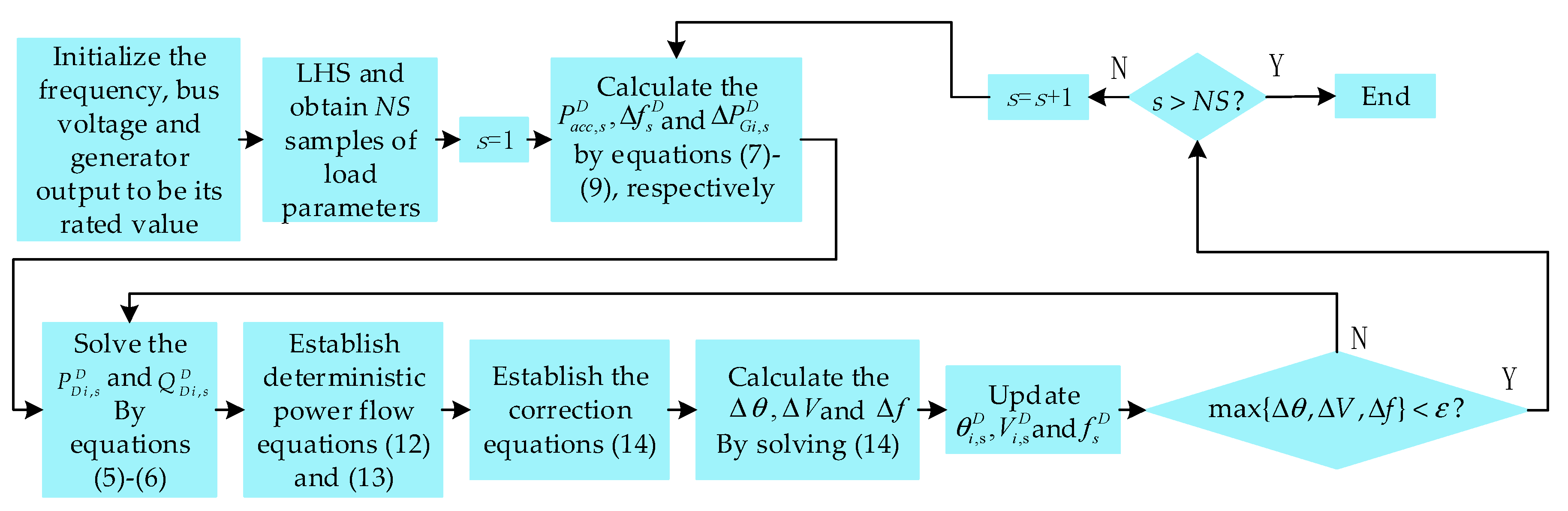
4. Case Study

The modified 39-bus New England system is selected as the test system, and the details of the relevant parameters are accessible from MATPOWER 6.0 [24]. In order to facilitate the simulation and analysis, a few modifications have been made to the original test system, with the conventional generators at bus 36 and 37 being replaced with wind power generators and their correlation coefficient being 0.8. Bus 38 is the access point of the DC system, and its transmission power is 1000 MW. Note that the part of the power higher than the original generator output of bus 38 is distributed to each load bus by increasing its expected load at the rated condition. The maximum active power output of the generator at the swing bus is changed to 800 MW, and the maximum active power output of the traditional generator at other buses is changed to 1.05 times its original value.

The predicted wind power output may follow a normal distribution [25] or beta distribution [26,27]. The mean and standard deviation are the rated value and 8% of the rated value, respectively, for the normal distribution. For the beta distribution, the wind power output is normalized according to the rated value; the corresponding shape and scale parameters are 16 and 1, separately. It is assumed that the power factor of the wind power output remains unchanged before and after the fluctuations. The parameter values of the load model are obtained from [16], and they all followed normal distributions with their means and standard deviations, as listed in

Table 2. The mean and standard deviation of the load parameters.

Load Parameters	${\mathit{k}}_{\mathit{p}\mathit{v}}$	${\mathit{k}}_{\mathit{q}\mathit{v}}$	${\mathit{k}}_{\mathit{p}\mathit{f}}$	${\mathit{k}}_{\mathit{q}\mathit{f}}$
mean	0.67	1.35	3.25	1
standard deviation	0.66	1.12	0.98	1.1

. The rated output of the traditional generator is set at its initial value from MATPOWER 6.0. The per unit value of ${\mathrm{k}}_{\mathrm{G}\mathrm{i}}$ of the generator at the swing bus is 18, and that of the other generators is 15. In addition, the inertia time constant ${\mathrm{T}}_{\mathrm{Ji}}$ of each generator varies normally in the interval [6,10], and hence the specific values of the generators are shown in

Table 3. The values of the inertia time constants of the generators.

Bus. No	30	31	32	33	34	35	39
$T_{J }$(s)	8.91	8.23	8.20	6.51	7.66	7.13	8.10

. All the tests are implemented in MATLAB [28].

4.1. Influence of Static Characteristics of Load Model on Actual Load under Normal Operation State

To illustrate the influence of the static frequency/voltage characteristics of the load and the change of the load compositions on the actual load, take the normal operation state as an example. The load models S0–S4 in

Table 4. The different stochastic load models.

Load Models	Specific Definition
S0	${\tilde{P}}_{Di}={\tilde{P}}_{DNi}$
S1	${\tilde{P}}_{Di}={\tilde{P}}_{DNi}(1+k_{pfi}(\tilde{f}-f_N))$
S2	${\tilde{P}}_{Di}={\tilde{P}}_{DNi}{({\tilde{V}}_i/V_{Ni})}^{k_{pvi}}$
S3	${\tilde{P}}_{Di}={\tilde{P}}_{DNi}{({\tilde{V}}_i/V_{Ni})}^{k_{pvi}}(1+k_{pfi}(\tilde{f}-f_N))$
S4	${\tilde{P}}_{Di}={\tilde{P}}_{DNi}{({\tilde{V}}_i/V_{Ni})}^{{\tilde{k}}_{pvi}}(1+{\tilde{k}}_{pfi}(\tilde{f}-f_N))$

are adopted to determine the actual load, with the fluctuations of the wind power not being taken into account. The load model S0 only considers the randomness of the rated load. On the basis of S0, the load models S1 and S2 take into account the static frequency and voltage characteristics of the load, respectively. Load model S3 considers both the static frequency and voltage characteristics of the load based on S0. Load model S4 considers the change of the load composition based on S3.

It is assumed that the standard deviation of the rated load distribution is 2% of$P_{DNi}$ [14], after which the corresponding samples can be produced by means of LHS. The distribution parameters of the actual total load as shown in

Table 5. The distribution parameters of the actual total load with the different load models S0–S4.

	Models	S0	S1	S2	S3	S4
Statistics
mean (MW)		6424.23	6423.96	6425.90	6425.65	6425.88
standard deviation (MW)		103.77	82.83	102.59	82.27	82.25
max (MW)		6786.49	6710.10	6778.79	6704.43	6699.74
min (MW)		6122.68	6181.25	6131.07	6187.98	6188.65

, corresponding to the load of the models S0–S4, are obtained by the method in Section 2.2.

As can be seen from Table 5, the actual load distributions obtained by the diverse load models are different, even at a normal operation state. The differences of the mean values for each load model are small, while the differences of the standard deviations are large. If the load distribution of model S0 is taken as the benchmark, the differences of the mean values for S1–S4 and for S0 are less than 0.026%, while the differences of the standard deviations can decrease by 20.74%. Therefore, the influence of the static characteristic parameters on the actual load distribution can be determined according to the decreasing proportion of the standard deviation compared to that of S0. When the static frequency and voltage characteristics of the load are considered separately, the differences of the standard deviations are 20.18% and 1.14%, respectively; and this value increases to 20.72% when both the static frequency and voltage characteristics are included, while the value for the load model S4 is 20.74%. This indicates that both the static frequency and voltage characteristics of the load can reduce the standard deviation of the actual load distribution, but the influence of the former is greater. Moreover, considering the static frequency and voltage characteristics of the load at the same time can further reduce the standard deviation of the actual load distribution. That is to say, under normal circumstances, the static characteristics of the load have a depressing effect on the degree of the actual load variation. In addition, the differences of the standard deviations of the actual load distributions between the load models S3 and S4 are very small, which indicates that when the operation state of the system changes a bit, the change of the load composition has little impact on the actual distribution of the load.

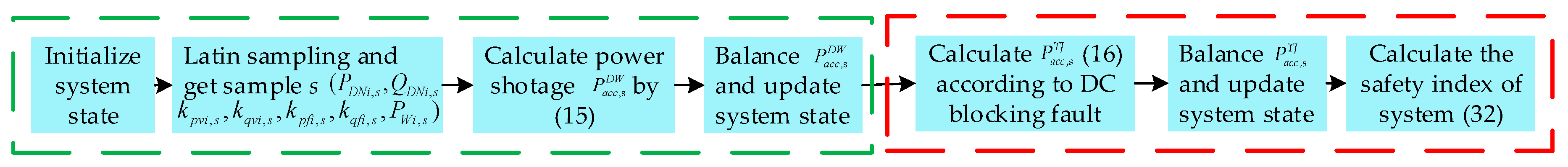
4.2. Influence of Parameters of Load Model and Wind Generation on the Actual Power Shortage after DC Blocking Fault

To analyze the influence of the probabilistic parameters of the load model and wind power output on the actual total power shortage after the DC block fault, different parameters are adopted. The power shortage can be obtained after the DC block fault by the load model S4 with the load parameter values in Table 2, and the inertia effects of the generators are considered, which is regarded as the base case.

4.2.1. Influence of the Randomness of Rated Load and Wind Generation on the Power Shortage

To analyze the influence of the randomness of the rated load and wind power output on the power shortage, different standard deviations of the rated load and different distributions of the wind power output are adopted. The standard deviations are set as 2%, 4%, 6% and 8% of its expected value at the rated condition, respectively; and normal and beta distributions are adopted to describe the wind power output for the latter when the other conditions are identical to the base case. The power shortage distributions are shown in Figure 3, where Figure 3a corresponds to the randomness of the rated load, while Figure 3b corresponds to the randomness of the wind power output.

It can be seen from Figure 3a that the standard deviation changes of the rated load have little impact on the actual power shortage of the system after the DC blocking fault; meanwhile, the distributions of the power shortage are almost the same in Figure 3b, even if the distributions of the wind power output are different. In addition, the distributions of the power deficiency in Figure 3 after the fault are all similar to the normal distributions, with mean values appearing at the vicinity of 800 MW. For Figure 3a, the more the standard deviation of the rated load increases, the flatter the distribution curve of the power deficiency is, that is, the larger the standard deviation and range of the power deficiency distribution are. Generally, the disturbances of the power system, namely the fluctuations of the wind power and rated load, have a slight impact on the power shortage distributions after the DC blocking fault, which can be explained by the fact that these disturbances have been dealt with before the DC blocking fault. Therefore, the system disturbances can only change the operation state before the fault, so that the effects of the system disturbances on the power shortage are negligible compared with the one caused directly by the DC blocking fault.

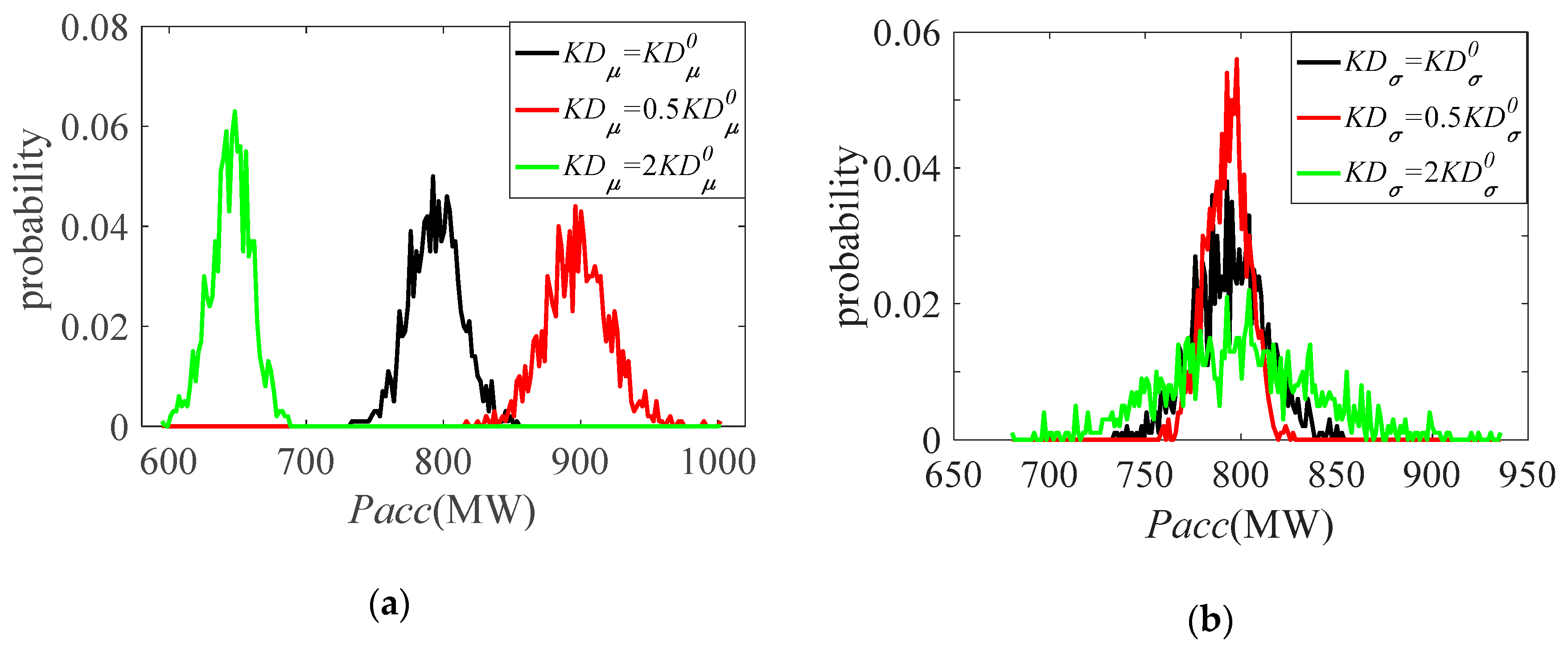
4.2.2. Influences Arising from Static Characteristics of Load on the Power Shortage

To illustrate the influences of the load static characteristics on the power shortage after the DC blocking fault, the load parameters ${\tilde{k}}_{pvi}$, ${\tilde{k}}_{qvi}$, ${\tilde{k}}_{pfi}$ and ${\tilde{k}}_{qfi}$ are changed, after which the power shortage after the fault can be determined correspondingly. In this paper, the mean and standard deviation sets of the load parameters are denoted as ${KD}_{\mu }$ and${KD}_{\sigma }$, respectively, which can be represented by Equations (33) and (34), and they are set as 0.5 and 2 times the original values separately to analyze their impact on the power shortage:

$$K{D}_{\mu }={[k_{pv1}{k}_{qv1}{k}_{pf1}{k}_{qf1},\dots ,k_{pv{N}_d}{k}_{qv{N}_d}{k}_{pf{N}_d}{k}_{qf{N}_d}]}^T,$$

(33)

$$K{D}_{\sigma }={[{\sigma }_{kpv1}{\sigma }_{kqv1}{\sigma }_{kpf1}{\sigma }_{kqf1},\dots ,{\sigma }_{kpv{N}_d}{\sigma }_{kqv{N}_d}{\sigma }_{kpf{N}_d}{\sigma }_{kqf{N}_d}]}^T.$$

(34)

It can be seen from Figure 4 that the variation of the load parameters will lead to the distribution change of the power shortage after the fault. The smaller the expectation and standard deviation of the power shortage are, the larger the ${KD}_{\mu }$ after the fault is. When the ${KD}_{\sigma }$ varies, the expected value of the power shortage after the fault is almost the same, while the standard deviation of the power shortage increases with the ${KD}_{\sigma }$. The system frequency and the bus voltage will drop after the DC blocking fault, and hence the actual load will decrease, as seen in Equation (5) of the load model, which results in the actual power shortage being lower than the power lost by the DC line. The larger the ${KD}_{\mu }$ is, the larger the actual load varies with the operation state of the system; consequently, the smaller the actual load and the expectation of the power shortage are after DC blocking. The larger the ${KD}_{\sigma }$ is, the larger the interval corresponding to the actual load distribution is, and the larger the interval and variance corresponding to the actual power shortage distribution are. By comparing the power shortage distribution in Figure 4a,b, the influence of the changes in ${KD}_{\mu }$ on the power shortage distribution is more significant than that of ${KD}_{\sigma }$. In general, the changes of ${KD}_{\mu }$ and ${KD}_{\sigma }$ are achieved according to the distribution of the load parameters, hence determining the actual distribution of the total system load and power shortage after the fault.

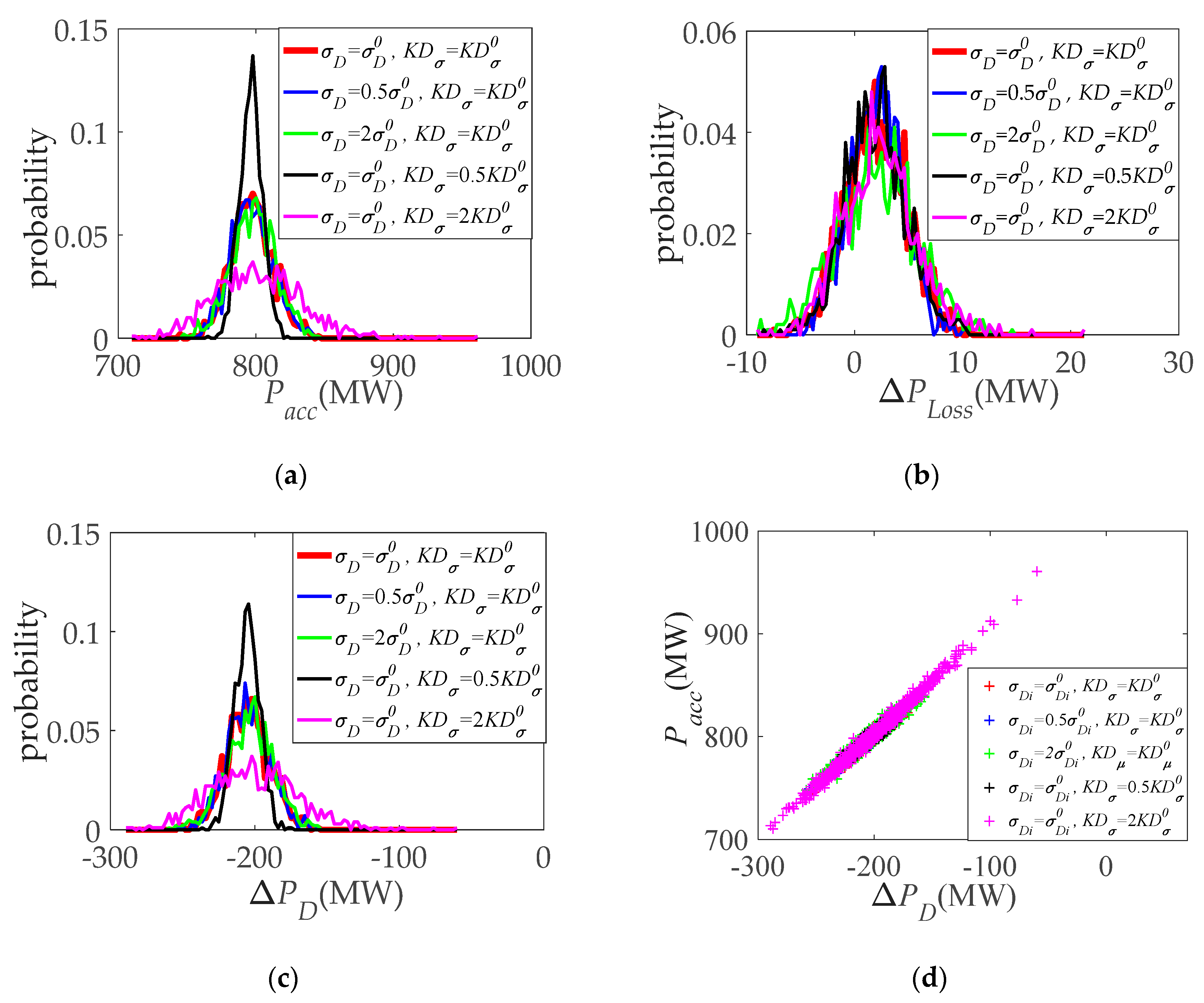
4.2.3. Comparison of the Effect of the Randomness of Rated Load and Static Characteristics on Actual Power Shortage

To compare the influences of the randomness of the rated load and load static characteristics on the power shortage after the DC blocking fault, Figure 5a shows the distributions of the power shortage with different ${\sigma }_D$ and ${KD}_{\sigma }$ values. It is assumed that ${\sigma }_D$ and${\sigma }_D^0$ represent the standard deviation set and the original standard deviation set of the rated load in the power system, respectively.

It can be seen from Figure 5a that the changes of ${KD}_{\sigma }$ have a greater impact on the power shortage than the changes of ${\sigma }_D$ do, which is consistent with the conclusions obtained by combining Figure 3a and Figure 4b. The actual power deficiency after the fault is mainly related to the power lost by the DC line, the change of the power loss and the actual load before and after the fault via Equation (22). The power lost by the DC line is a determined value in this paper. Therefore, to further analyze the influences of ${\sigma }_D$ and ${KD}_{\sigma }$ on the actual power shortage, their influences on the change of the system power loss and on the actual load before and after the fault are analyzed separately, as shown in Figure 5b,c, respectively.

As can be seen from Figure 5b, the change of the power loss with different ${\sigma }_D$ and ${KD}_{\sigma }$ values before and after the fault is negligible compared to the power lost by the DC blocking fault. The change of ${KD}_{\sigma }$ has a greater impact on the actual load variation than the change of ${\sigma }_D$ does, as shown in Figure 5c. This indicates that the actual power shortage after the DC blocking is mainly related to the change of the actual load, except for the power lost by the DC line itself. This conclusion can be further proven by the approximate linear relation between the actual power shortage and the change of the actual load in Figure 5d, regardless of test scenarios. The static characteristics of the load are directly related to the load variation. Therefore, in order to obtain the accurate estimation of the actual power shortage, the values of the load parameters in the load model need to be exactly determined.

4.3. Influence of Inertia Effect on Actual Power Shortage

The power shortage after the fault is immediately balanced if the inertia effect of the generator is neglected, and in this condition the power shortage is just the power lost by the DC line, which is 1000 MW in this paper. The power shortage distribution of the system after the fault is shown in the black curve of Figure 4, taking into account the inertia effect. The role of the inertia effect of the generator is to calculate the operation state accurately, before the response of the generator and the load-shedding device after the fault, so as to accurately estimate the power deficiency. The power deficiency of the system after the fault is determined by Equation (16). 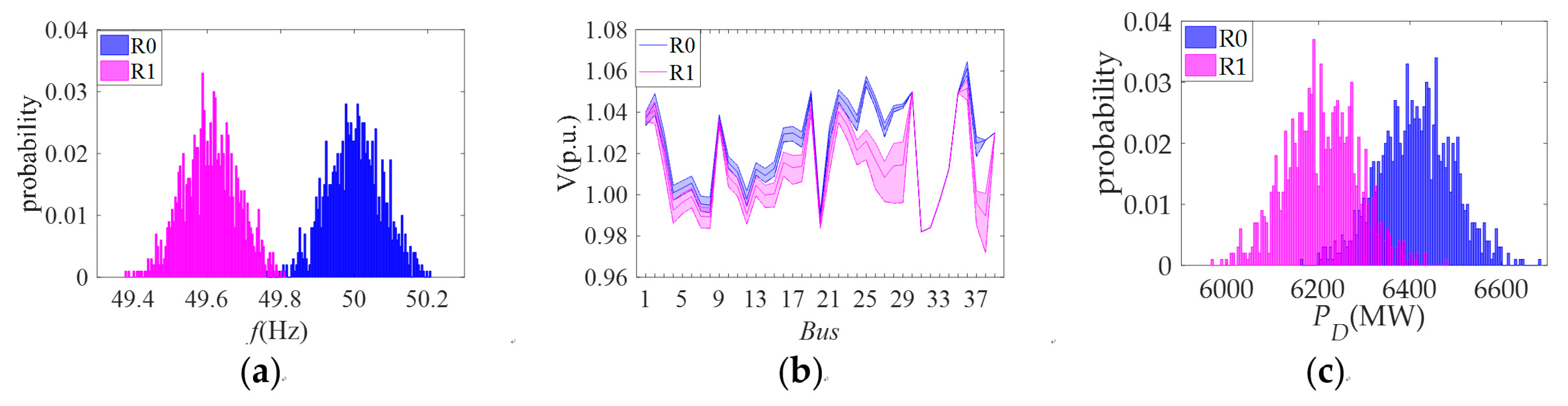The output of the generator at the inertia effect stage is the same as that before the fault, and the power loss will not change greatly in the system state, as shown in Figure 5b; consequently, the solution of the power shortage mainly focuses on the accurate solution of the actual load after the fault. To illustrate the role of the inertia effect of the generator in accurately solving the power shortage after the fault, the distributions of the frequency, bus voltage and actual load are calculated, respectively, regardless of whether the inertia effect is considered or not, and their distributions are shown in Figure 6.

The system frequency and bus voltage after the fault are the same as before the fault when the inertia effect is not considered, corresponding to R0 in Figure 6a,b. When the inertia effect of the generator is taken into account, the frequency and the voltage magnitude of PQ bus decrease, corresponding to R1 in Figure 6a,b. Figure 6c shows that there is a significant difference in the actual load, when the inertia effect of the generator is taken into account after the fault, which is closely related to the change of the system operation state and is consistent with the results in Figure 6a,b. It is worth mentioning that with diverse system states the actual load and power loss of the system are different, according to Equations (5) and (21), leading to different power deficiency values according to Equation (16). It can be verified that the operation states after the fault can be calculated accurately by considering the inertia effect of the generators, so that the power shortage can also be determined more accurately.

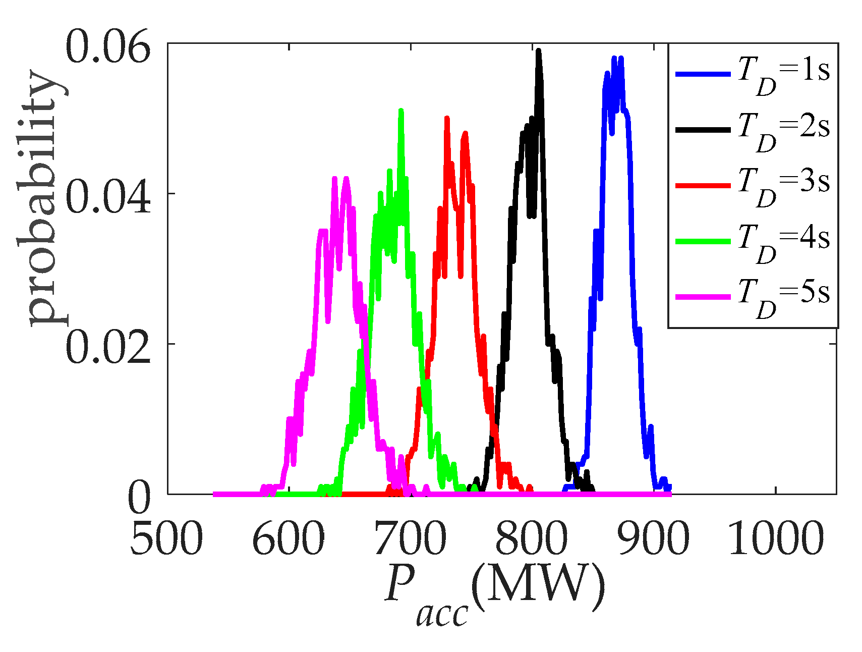
The high power deficiency after the fault needs to be balanced in time, and its response speed will affect how to balance the power deficiency. The accurate calculation of the power deficiency can determine effective countermeasures against its emergence, so that the system can quickly return to the normal state, and vice versa. In fact, the inertia effect of the generator exists during the response delay of the actual system, so there is a significant error of the power shortage when the inertia effect of the generator is not taken into account. Therefore, it is necessary to introduce the inertia effect of the generator to calculate the accurate power deficiency for the high power imbalance fault. To further illustrate the role of the inertia effect of the generator, the response delay time $T_D$ is changed to obtain the distribution of the actual power deficiency in Figure 7.

The actual power deficiency of the system decreases with the increase of the delay time $T_D$. This is because, as the delay time $T_D$ increases, the system frequency and bus voltage drop more, resulting in a smaller actual load of the system, so that the power shortage is smaller. It is worth noting that the total load shedding would be smaller with a larger response delay. However, the frequency and bus voltage dropping too much may cause the relay protection to act, or may even result in a collapse of the system and voltage. Therefore, the system response delay $T_D$ should be set according to the practical situation of the system.

4.4. Determination of Load-Shedding Strategy Scheme

To illustrate the influence of the different load shedding schemes on the system security after the DC blocking fault, the load-shedding coefficients of each bus, according to Section 3.3, are used to obtain the security index of the system after the fault. When the load-shedding coefficients ${\alpha }_{PDi,s}^{M1}$, ${\alpha }_{PDi,s}^{M2}$ and ${\alpha }_{PDi,s}^{M3}$ are employed, the corresponding security index values are 31.3423, 26.7135 and 11.8081, calculated individually via Equation (32). 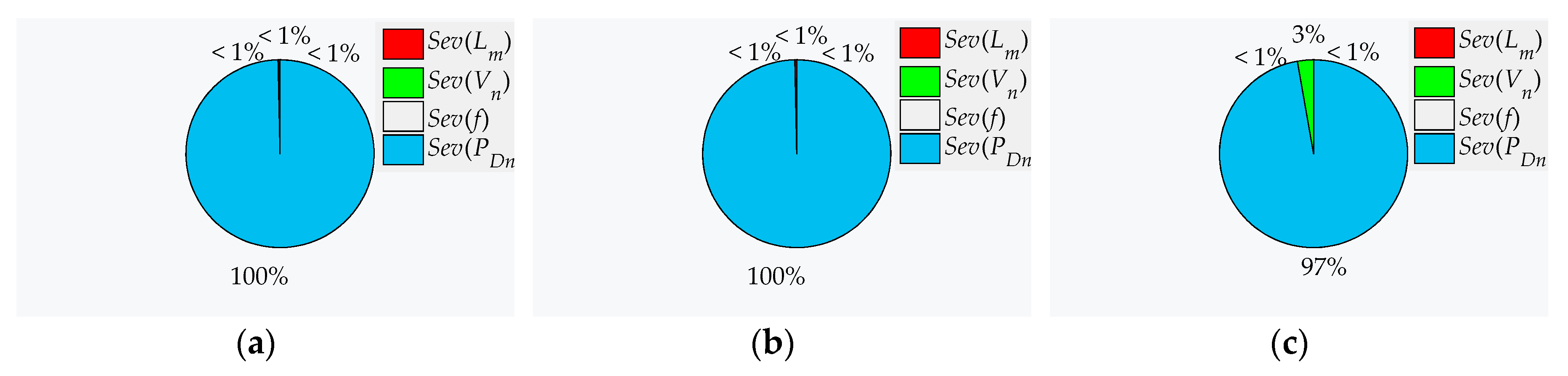To validate the effectiveness of the new security index proposed in Section 3.4, the compositions of the comprehensive security index Sev with different load-shedding coefficients are shown in Figure 8. It can be seen from Figure 8 that no matter which load-shedding coefficient is adopted, the severity of the load distribution shifting ${Sev(P}_D)$ contributes to the main block to the system safety index. On the one hand, this result shows that the introduction of the load-shifting severity index plays an intuitive and important role in the system safety index. On the other hand, it indicates that the voltage magnitude, frequency and branch power can be guaranteed to slightly exceed the limit or not exceed it at all via the use of the load-shedding strategy after the fault, which also benefits from the accurate determination on the power deficiency in the previous step.

It is worth mentioning that different load-shedding schemes have different influences on the steady-state security of the receiving-end system after the fault, while the load-shedding coefficient corresponding to M3 makes the system have the best security level after the fault. This is because the load-shedding coefficient determined by the PF tracing results can result in the load that is majorly supplied by the blocking line being cut, thus leading the system state to change less after the fault compared to other load-shedding coefficients. Therefore, after accurately solving the total power shortage, it is necessary to adopt a more reasonable load-shedding strategy to keep the system more secure. 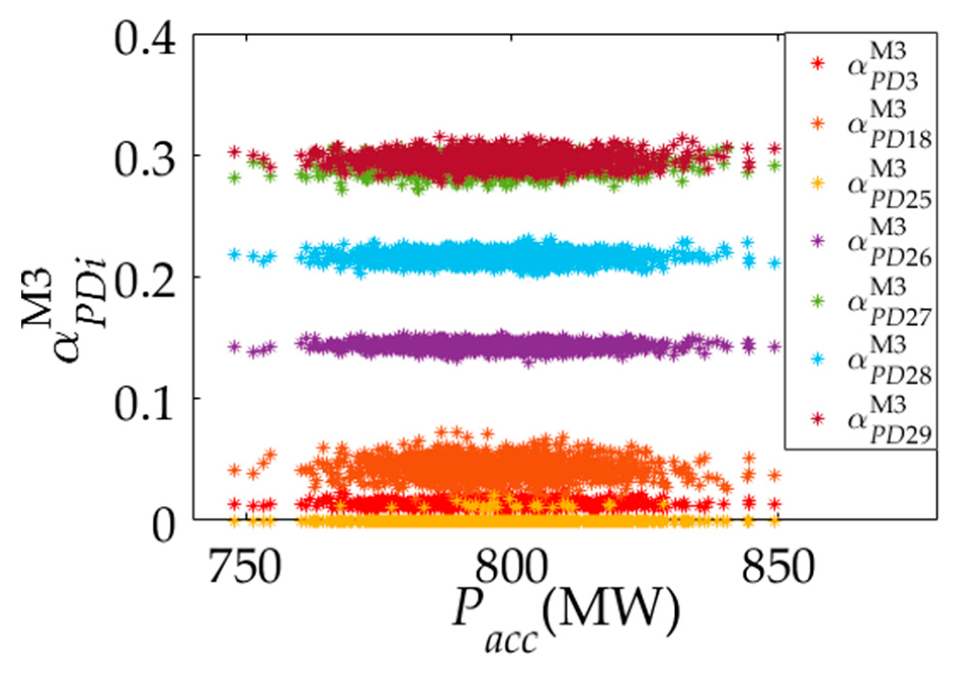To further simplify the ${\alpha }_{PDi,s}^{M3}$, the relationships between the ${\alpha }_{PDi,s}^{M3}$ and the actual power shortage of the system are analyzed, as shown in Figure 9.

As can be seen from Figure 9, if the actual power deficiency of the whole system varies in the stochastic context, the load-shedding coefficient of the same bus could be different. Even if the actual power deficiency is the same, the load-shedding coefficient of the same bus will be different due to the different operation states of the system. However, the change of the load-shedding coefficient, along with actual power deficiency for the same bus, is small and can be treated as a constant, but this is not investigated in the other two load shedding strategies where ${\alpha }_{PDi,s}^{M1}$ and ${\alpha }_{PDi,s}^{M2}$ are adopted. The load shedding coefficients for M3 remaining approximately constant values can be explained by the fact that the PF tracing result of each load bus varies almost linearly with the power deficiency, which leads to the unchanged value of ${\alpha }_{PDi,s}^{M3}$ for the different samples. Therefore, the expectation of the load-shedding coefficient ${\overline{\alpha }}_{PDi}^{M3}$ is adopted for the different actual power deficiencies under the stochastic context. In addition, the security index of the system is 11.9091 when ${\overline{\alpha }}_{PDi}^{M3}$ is used as the load-shedding coefficient. This shows that the system security is still basically unchanged when ${\overline{\alpha }}_{PDi}^{M3}$ is adopted as the load-shedding coefficient as compared to ${\alpha }_{PDi,s}^{M3}$, but more importantly the deterministic coefficients achieved for the load-shedding strategy are more practical.

5. Conclusions

In this paper, an emergency load-shedding strategy for the DC blocking fault of a hybrid AC/DC receiving-end system grid is proposed, taking into account the static frequency and voltage characteristics of the stochastic load model. The new stochastic load model, which considers the randomness of the rated load and the load compositions with static frequency/voltage characteristics, is more practical than the traditional load model. Through the analysis of the load model, it can be found that both the static frequency and voltage characteristics of the load have a depressing effect on the randomness of the load, while the effect of the former one is more obvious. Therefore, the introduction of the static frequency and voltage characteristics of the load, including their distributions, makes the actual load and power shortage estimation after the fault more accurate. After the DC blocking fault, the inertial effect of the generator is introduced to accurately determine the operation state after the fault; thus, the actual power deficiency can be obtained by updating the actual load and power loss of the system.

The experimental analysis indicates that there are many factors affecting the actual power shortage after the fault. Among them, the static characteristics of the load and the system response delay time have the most significant influence, while the fluctuations of the wind power and rated load have a slight influence. In detail, the response delay of the system makes the operation state vary, leading to a power loss change; furthermore, the static characteristics of the load make the actual load vary with the operation state. The combination of the response delay and load static characteristics results in the actual power imbalance being smaller than the power lost by the DC blocking line, which is more practical compared to the existing method. Therefore, in order to obtain the accurate power imbalance after the fault, it is necessary to establish an accurate load model and calculate the operation state exactly, especially to accurately determine the load parameters for the load model.

In addition, this paper also puts forward a comprehensive evaluation index of the system security, more comprehensive than the traditional security index, and which not only takes into account the traditional off-limit situations of the bus voltage and branch but also the off-limit situation of the frequency and load offset degree. The security index of the system is used to compare different load-shedding schemes and select the load-shedding scheme with the best performance. Under the basic premise of not deteriorating the system security, the load-shedding coefficients of the loads, corresponding to the proposed load-shedding strategy for different power shortages, are unified in this paper, so as to make the load-shedding strategy more practical.