Phase Space Reconstruction Algorithm and Deep Learning-Based Very Short-Term Bus Load Forecasting

Abstract

With the refinement and intelligence of power system optimal dispatching, the widespread adoption of advanced grid applications that consider the safety and economy of power systems, and the massive access of distributed energy resources, the requirement for bus load prediction accuracy is continuously increasing. Aiming at the volatility brought about by the large-scale access of new energy sources, the adaptability to different forecasting horizons and the time series characteristics of the load, this paper proposes a phase space reconstruction (PSR) and deep belief network (DBN)-based very short-term bus load prediction model. Cross-validation is also employed to optimize the structure of the DBN. The proposed PSR-DBN very short-term bus load forecasting model is verified by applying the real measured load data of a substation. The results prove that, when compared to other alternative models, the PSR-DBN model has higher prediction accuracy and better adaptability for different forecasting horizons in the case of high distributed power penetration and large fluctuation of bus load.

1. Introduction

Electricity cannot be stored in large quantities, and the investment recovery cycle of large-scale energy storage equipment is long. Therefore, in order to ensure the safe operation of power systems and power quality on the user side, the operators must have knowledge of future power loads [1]. Power system load forecasting is an important method to understand the trend of future electric load. In addition, power load forecasting is of great significance for the planning of power systems and scheduling of generation and transmission maintenance. Power system load forecasting is generally divided into long-term forecasting, medium-term forecasting, short-term forecasting, and very short-term forecasting [2]. Among them, short-term load forecasting (STLF) and very short-term load forecasting (VSTLF) are of great significance for economic dispatch, optimal power flow, and electricity market trading. The higher the accuracy of load forecasting is, the more beneficial it is to improve the utilization rate of power generation equipment and the effectiveness of economic dispatch, and reduce the operation cost of smart grid.

In the past decades, experts and scholars have made systematic and effective research on traditional deterministic and probabilistic STLF and VSTLF. Deterministic forecasting methods can be divided into two main categories [3]: The first category uses statistical forecasting models, such as linear regression [4], curve extrapolation [5], Autoregressive Integrated Moving Average (ARIMA) model [6,7], and other time series methods; the second category uses artificial intelligent forecasting models, such as Bayesian estimation [8], Random Forests [9], Support Vector Regression (SVR) [10,11], Artificial Neural Network (ANN) [12,13], Deep Belief Network (DBN) [14,15], and Long Short Term Memory (LSTM) Network [16,17]. These methods have achieved high forecasting accuracy and good robustness in day-ahead and hour-ahead load forecasting. However, most of the studies are focused on system-level load forecasting and there are relatively few on bus load forecasting. Generally, bus loads can refer to loads supplied by transmission and distribution systems transformers [18]. Bus load forecasting can be conducive to the optimal scheduling of decentralized generation, network congestion studies, and others [19].

With the refinement and intelligence of power grid optimal dispatching and the wide application of advanced smart grid applications, which take into account the security and economy of power system, the demand for bus load forecasting accuracy is increasing. Since bus load base is much smaller than that of a system, the uncertainty of bus load and the multi-dimensional nonlinearity [20] are more obvious. The traditional method of distributing the predicted value of system through bus load ratio often fails to achieve satisfactory results [21]. In this regard, the literature [18] modifies the ANN model for the aggregated load of the interconnected system and proposes two novel hybrid forecasting models, which can capture and successfully treat the special characteristics of bus load patterns. In Ref. [19], a bus load forecasting model based on clustering and ANN is proposed; the day-ahead load forecasting and hour-ahead load forecasting are carried out, achieving high prediction accuracy.

With a large number of distributed power access, the uncertainty and nonlinear characteristics of system [22] and bus load are further enhanced. As the collection time interval of distributed photovoltaic power, plant data is generally several minutes. The short-term and day-ahead load forecasting in hours of bus cannot make full use of historical information and have low prediction accuracy. In order to ensure the reliable operation of power system real-time security analysis and economic dispatch, more detailed VSTLF is needed. The authors of [23] proposed a chaotic-radial basis function (RBF) photovoltaic power generation prediction model and verified its prediction accuracy under different weather conditions. However, the author only validated the prediction accuracy of the model in the case of single-step prediction and did not involve the forecasting horizon problem of the model [24]. Ref. [20] proposes a novel load forecasting model based on phase space reconstruction (PSR) algorithm and bi-square kernel (BSK) regression, and achieves high prediction accuracy on different data sets. However, after phase space reconstruction, different BSK models are used to independently predict the various dimensional data, which neglect the time series characteristics of the load.

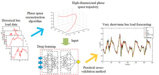
In view of the shortcomings of the above forecasting model, considering the adaptability to different forecasting horizons, the time series characteristics of load, and the volatility brought by large-scale access of new energy sources, this paper proposes a novel very short-term bus load forecasting model based on phase space reconstruction and deep belief network (PSR-DBN). Because the amount of historical data in VSTLF is relatively large and closely related to future load trend, the impact of weather, electricity price, and other factors on VSTLF is not considered in this paper. Firstly, the proposed PSR-DBN model performs phase space reconstruction on bus load history data, and projects the historical data to the motion track of a moving point in the phase space. Then the model takes advantage of the excellent nonlinear fitting ability of the deep belief network to fit the moving point trajectory and provide a prediction of the trajectory. Finally, the predicted value of the load is obtained. At the same time, the structure of the DBN is optimized by cross-validation. In order to test the validity and superiority of the proposed PSR-DBN very short-term bus load forecasting model, this paper applies the measured load data of a substation in China to verify the forecasting effectiveness of the model under different forecasting horizons (5 min–1 h). In addition, other six alternative forecasting models are employed to further compare with the proposed PSR-DBN model.

The major contributions of this paper are as follows:

• A novel hybrid VSTLF model based on phase space reconstruction ensemble deep belief network is proposed, which can maintain high prediction accuracy in the case of high distributed power penetration and large fluctuation of bus load.
• The Levenberg-Marquardt backpropagation (LMBP) algorithm is used to fine-tune the DBN, which can make DBN convergence faster and more accurate, compared with a BP algorithm.
• A practical method based on cross-validation is proposed to tune the structure of DBN for better forecasting performance.
• The PSR algorithm is adopted to make a regular pattern that could not be obtained in one-dimensional time series appear in a high-dimensional phase space, which improves the adaptability of a forecasting model to different forecasting horizons, especially long estimation.

The rest of this paper is organized as follows. In Section 2, the relevant theory of the PSR-DBN model is introduced. Section 3 provides the principal steps of the PSR-DBN model and covers the tuning method of network hyperparameter based on cross-validation. Section 4 presents the evaluation criteria of forecasting accuracy, case study settings, forecasting results, and a comparison. Section 5 gives the conclusion of the paper and an outlook for future research.

2. Methodology

2.1. Phase Space Reconstruction (PSR)

Phase space reconstruction (PSR) is an efficient method for analyzing nonlinear time series. The basic idea of phase space reconstruction is to regard the time series as a component generated by a nonlinear dynamic system. The variation law of the component can reconstruct the equivalent high-dimensional phase space of the dynamic system, and the time series can be projected into a moving point trajectory in the high-dimensional phase space. If there is a one-dimension time series $\mathit{x}=\left\{x_1,x_2\cdots x_N\right\}$, the embedding dimension is m, and the delay time is t, then the set of time series reconstructed by phase space can be expressed as:

$$\left[\begin{array}{c}{X}_1\\ X_2\\ ⋮\\ X_M\end{array}\right]=\left[\begin{array}{cccc}{x}_1& x_{1+t}& \cdots & x_{1+(m-1)t}\\ x_2& x_{2+t}& \cdots & x_{2+(m-1)t}\\ ⋮& ⋮& \cdots & ⋮\\ x_M& x_{M+t}& \cdots & x_N\end{array}\right]$$

(1)

where $M=N-(m-1)t$.

The key to PSR is to determine the optimal embedding dimension m_opt and optimal delay t_opt. In this paper, the C-C method [25] is employed to determine the optimal embedding dimension m_opt and delay t_opt at the same time.

Based on Equation (1), the associated integral is defined as:

$$C\left(m,N,r_k,t\right)=\frac{2}{M\left(M-1\right)}{\displaystyle \sum _{1\le i<j\le M}\theta \left(r_k-\Vert X_i-X_j\Vert \right)}$$

(2)

where $\theta \left(x\right)=\{\begin{array}{c}\begin{array}{cc}0& x<0\end{array}\\ \begin{array}{cc}1& x\ge 0\end{array}\end{array}$.

According to BDS (Brock-Dechert-Scheinkman) statistical conclusions [26,27], when $N>3000$, the range of values of m and r_k can be obtained, $m\in \left\{2,3,4,5\right\}$, $r_k=k\times 0.5\sigma$, where $\sigma$ is the standard deviation of the time series and $k\in \left\{1,2,3,4\right\}$.

Based on matrix partitioning average strategy, the test statistics $S$ is defined as:

$$S\left(m,N,r_k,t\right)=\frac{1}{t}{\displaystyle \sum _{i=1}^t{C}_i\left(m,\frac{N}{t},r_k,t\right)-C_i^m}\left(m,\frac{N}{t},r_k,t\right)$$

(3)

For $N\to \infty$, Equation (3) can be deformed to:

$$S\left(m,r_k,t\right)=\frac{1}{t}{\displaystyle \sum _{i=1}^t{C}_i\left(m,r_k,t\right)-C_i^m}\left(m,r_k,t\right)$$

(4)

For the fixed m and t, $S\left(m,r_k,t\right)$ will equal for 0 for all r, if the data are iid and $N\to \infty$. However, the real data set is not infinite, and there may be a correlation between data. Thus, the optimal delay time may be either the zero crossing of $S\left(m,r_k,t\right)$ or the times at which $S\left(m,r_k,t\right)$ shows the least variation with r [25].

To represent the variation of $S\left(m,r_k,t\right)$ with r, the test statistics $\Delta S$ is defined as:

$$\Delta S\left(m,t\right)=\max \left[S\left(m,r_{k_1},t\right)\right]-\min \left[S\left(m,r_{k_2},t\right)\right]$$

(5)

where $k_1\in \left\{1,2,3,4\right\}$, $k_2\in \left\{1,2,3,4\right\}$.

The means of $S$ and $\Delta S$ are defined as $\overline{S}$ and $\overline{\Delta S}$, and the equations are shown as:

$$\{\begin{array}{l}\overline{S}\left(t\right)=\frac{1}{4\times 4}{\displaystyle \sum _{m=2}^5{\displaystyle \sum _{k=1}^{4}S\left(m,r_k,t\right)}}\\ \overline{\Delta S}\left(t\right)=\frac{1}{4}{\displaystyle \sum _{m=2}^5\Delta S\left(m,t\right)}\end{array}$$

(6)

For all values of t, $\overline{S}\left(t\right)$ and $\overline{\Delta S}\left(t\right)$ can find corresponding values. Wherein, the t value corresponding to the first zero point of $\overline{S}\left(t\right)$ or the first minimum point of $\overline{\Delta S}\left(t\right)$ is rounded to be the optimal delay t_opt.

The test statistic $S_{cor}$ is defined as:

$$S_{cor}\left(t\right)=\overline{\Delta S}\left(t\right)+\left|\overline{S}\left(t\right)\right|$$

(7)

where the t value corresponding to the global minimum point of $S_{cor}\left(t\right)$ is the optimal embedded window $t_{\omega }$.

When the optimal delay t_opt is determined by Equation (6) and the optimal embedded window $t_{\omega }$ is determined by Equation (7), the optimal embedding dimension m_opt can be determined by rounding the value of Equation (8).

$$t_{\omega }=(m_{opt}-1)t_{opt}$$

(8)

2.2. Deep Belief Network (DBN)

The Deep Belief Network (DBN) is a deep learning model proposed by Geoffrey Hinton [28] in 2006 and is a stack of multiple Restricted Boltzmann Machines (RBM). Compared with the Artificial Neural Network (ANN), DBN employs pre-training technology combined with Backpropagation (BP) algorithm to solve network parameters. Therefore, it is not easy for DBN to fall into a local optimal solution and has higher convergence accuracy. Furthermore, when the number of layers and the number of neurons in each layer are large, DBN also has a fast convergence speed, which makes it more suitable for the fitting problem of complex nonlinear time series [29].

2.2.1. Restricted Boltzmann Machine (RBM)

The RBM consists of a visible layer V and a hidden layer H. As shown in Figure 1, the visible layer consists of n_v neurons and the hidden layer consists of m_h neurons, each of which takes a value of 0 or 1 and obeys the Bernoulli distribution, i.e., $v_i\in \left\{0,1\right\}\left(i=1,2\cdots n\right)$, $h_j\in \left\{0,1\right\}\left(j=1,2\cdots m\right)$. There is no connection between the neurons in each layer, and the neurons between the layers are connected by weights $\omega$.

RBM is a kind of probabilistic unsupervised learning. Its network parameters are composed of visible layer bias $b$, weight matrix $\mathsf{\omega }$, and hidden layer bias $c$, and the optimal value of network parameters is determined by the minimum energy function. The energy function is defined as:

$$E\left(v,h|\mathsf{\theta }\right)=-{\displaystyle \sum _{i=1}^n{b}_i{v}_i}-{\displaystyle \sum _{j=1}^m{c}_j{h}_j-{\displaystyle \sum _{i=1}^n{\displaystyle \sum _{j=1}^m{v}_i{\omega }_{ij}{h}_j}}}$$

(9)

where ${\omega }_{ij}$ is the connection weight of the i-th visible layer neuron and the j-th hidden layer neuron, and $\mathsf{\theta }=\left\{b,\mathsf{\omega },c\right\}$.

Based on Equation (9), the joint probability distribution of the visible neuron state and the hidden neuron state is shown as:

$$P\left(v,h|\mathsf{\theta }\right)=\frac{e^{-E\left(v,h|\mathsf{\theta }\right)}}{Z}$$

(10)

where normalization factor $Z={\displaystyle \sum _{v,h}{e}^{-E\left(v,h|\mathsf{\theta }\right)}}$, which represents the sum of the energy function negative exponents under all possible values of visible layer neuron state variable v and hidden layer neuron state variable h.

The probability distribution $P\left(v\right)$ of v can be derived from Equation (10) as:

$$P\left(v|\mathsf{\theta }\right)={\displaystyle \sum _h\frac{e^{-E\left(v,h|\mathsf{\theta }\right)}}{Z}}$$

(11)

Thus, the objective function of RBM training can be expressed as a likelihood function of the probability distribution of visible layer state variable v on the training set, and the likelihood function can be derived from the Equation (11) as:

$$L\left(\mathsf{\theta }\right)={\displaystyle \sum _{v\in T}\log P\left(v|\mathsf{\theta }\right)}$$

(12)

where T represents the set of sample inputs on the training set, and when the objective function takes the maximum value, the energy function is the minimum.

According to the network structure in Figure 1, the activation probability of $v_i$ in a given hidden layer neuron state $h$ and the activation probability of $h_j$ in a given visible layer neuron state $v$ can be derived as:

$$P\left(v_i=1|h\right)=\sigma \left(b_i+{\displaystyle \sum _{j=1}^m{\omega }_{ij}{h}_j}\right)$$

(13)

$$P\left(h_j=1|v\right)=\sigma \left(c_i+{\displaystyle \sum _{i=1}^n{\omega }_{ij}}{v}_i\right)$$

(14)

where $\sigma$ represents the sigmoid function, $\sigma \left(x\right)=\frac{1}{1+e^{-x}}$.

Since the gradient cannot be directly obtained when using stochastic gradient ascent algorithm to seek the maximum of Equation (12), the training of RBM usually applies Contrastive Divergence (CD) algorithm to approximate the gradient of likelihood function [30]. The specific steps of RBM training are as follows:

Step 1: Substitute the input of the training set as $v_1$ in Equation (14) to obtain $P\left(h_1=1|v_1\right)$, then employ random sampling to acquire the reconstructed value of $h_1$.

Step 2: Substitute $h_1$ in Equation (13) to obtain $P\left(v_2=1|h_1\right)$ and then employ random sampling to acquire the reconstructed value of $v_2$.

Step 3: Substitute $v_2$ in Equation (14) to obtain $P\left(h_2=1|v_2\right)$.

Step 4: Update network parameters. The iteration algorithm of network parameters is as follows:

$$\{\begin{array}{l}{\mathsf{\omega }}^{\left(k+1\right)}={\mathsf{\omega }}^{\left(k\right)}+\epsilon \left(h_1{v}_1^{\mathrm{T}}-P\left(h_2=1|v_2\right)v_2^{\mathrm{T}}\right)\\ b^{\left(k+1\right)}=b^{\left(k\right)}+\epsilon \left(v_1-v_2\right)\\ c^{\left(k+1\right)}=c^{\left(k\right)}+\epsilon \left(h_1-P\left(h_2=1|v_2\right)\right)\end{array}$$

(15)

where $\epsilon$ is the learning rate, which takes the value of 0.8 in this paper, and the superscript k represents the k-th iteration.

2.2.2. DBN based on Levenberg-Marquardt backpropagation (LMBP) Algorithm

Traditional DBN is formed by stacking multiple RBMs, in which the hidden layer of the previous RBM is used as the visible layer of the next RBM. CD algorithm is used to determine the network parameters layer by layer during pre-training, which is unsupervised learning. Then the pre-trained network parameters are assigned to the neural network as the initial training value of network parameters. The network parameters are fine-tuned by using the sample labels in the training set combined with BP algorithm, which is supervised learning. The structure of a traditional DBN is shown in Figure 2.

In this paper, the LM (Levenberg-Marquardt) BP algorithm [31] is used to replace the traditional BP algorithm to fine-tune the DBN. Compared with the traditional BP algorithm, the LMBP algorithm has faster convergence speed and higher convergence reliability, and is more suitable for training neural networks with many hidden layers and neurons.

Different from the traditional BP algorithm, the LMBP algorithm is based on the Gauss-Newton method in the least square solution. The square of error $v$ is taken as the objective function and the second-order Taylor expansion of objective function is derived. After approximating the gradient of the objective function (ignoring the high-order term), the correction of weight $\mathsf{\omega }$ is:

$$\Delta \mathsf{\omega }=-{\left[J^T\left(\mathsf{\omega }\right)J\left(\mathsf{\omega }\right)+\mu I\right]}^{-1}{J}^T\left(\mathsf{\omega }\right)v\left(\mathsf{\omega }\right)$$

(16)

where $\mu$ is the correction coefficient, which is set to prevent $J^T\left(\mathsf{\omega }\right)J\left(\mathsf{\omega }\right)$ from being irreversible; $I$ is the identity matrix; $J\left(\mathsf{\omega }\right)$ is the Jacobian matrix of $v\left(\mathsf{\omega }\right)$, which can be written as:

$$J\left(\mathsf{\omega }\right)=\left[\begin{array}{cccc}\frac{\partial v_1}{\partial {\omega }_1}& \frac{\partial v_1}{\partial {\omega }_2}& \cdots & \frac{\partial v_1}{\partial {\omega }_a}\\ \frac{\partial v_2}{\partial {\omega }_1}& \frac{\partial v_2}{\partial {\omega }_2}& \cdots & \frac{\partial v_2}{\partial {\omega }_a}\\ ⋮& ⋮& \ddots & ⋮\\ \frac{\partial v_a}{\partial {\omega }_1}& \frac{\partial v_a}{\partial {\omega }_2}& \cdots & \frac{\partial v_a}{\partial {\omega }_a}\end{array}\right]$$

(17)

where $\frac{\partial v_i}{\partial {\omega }_j}$ represents the partial derivative of $v_i$ to ${\omega }_j$.

Similar to BP algorithm, the modifier expression of weight ${\mathsf{\omega }}^{\left(k+1\right)}$ in the k-th iteration is:

$${\mathsf{\omega }}^{\left(k+1\right)}={\mathsf{\omega }}^{\left(k\right)}+\Delta {\mathsf{\omega }}^{\left(k\right)}$$

(18)

$\mu$ needs to be adjusted in each iteration to obtain a better convergence effect. When $\mu$ is small, the algorithm is standard Gauss-Newton method, which has higher convergence accuracy. However, if the difference between the objective function and the approximate quadratic function is too large in the iteration, the convergence effect will be poor. When $\mu$ is large, the algorithm becomes traditional BP algorithm. When the Gauss-Newton method has a poor convergence performance, the gradient descent BP algorithm can be used as an auxiliary solution.

3. PSR-DBN Forecasting Model

3.1. The Procedure of the PSR-DBN Model

For a list of bus load historical data time series $\mathit{p}=\left\{p_1,p_2\cdots p_N\right\}$, the prediction process of the PSR-DBN forecasting model is as follows:

Step 1 normalization: The load time series is normalized to prepare for the training of deep belief network, and the maximum and minimum values of data are saved for subsequent denormalization of the load predicted value to restore real value.

Step 2 PSR: The C-C method is adopted to process the load time series to find the optimal embedding dimension m and the optimal delay t of time series. Then the load time series is reconstructed according to the obtained embedding dimension m and delay t. The reconstructed load time series is as follows:

$$\left[\begin{array}{c}{p}_1\\ p_2\\ ⋮\\ p_M\end{array}\right]=\left[\begin{array}{cccc}{p}_1& p_{1+t}& \cdots & p_{1+(m-1)t}\\ p_2& p_{2+t}& \cdots & p_{2+(m-1)t}\\ ⋮& ⋮& \cdots & ⋮\\ p_M& p_{M+t}& \cdots & p_N\end{array}\right]$$

(19)

where $M=N-(m-1)t$.

Step 3 DBN: The DBN is constructed by using the phase space matrix in step 2 as the training set and employing cross-validation to optimize the hyperparameters of the network. The details of hyperparameters tuning are introduced in Section 3.2. Finally, the trained DBN is adopted to predict the load value of the future moment.

Step 4 denormalization: The load prediction value returned by the deep belief network in step 3 is denormalized by applying the maximum and minimum values saved in step 1, then the actual load forecasting value is obtained.

The flow chart corresponding to the above steps is shown in Figure 3:

3.2. Determination of DBN Network Structure

Similar to the neural network, DBN also has many hyperparameters to be set. The rationality of hyperparameters adjustment determines the prediction accuracy of the prediction model. Unreasonable hyperparameters will lead to a significant increase in prediction error. The determination of the network structure is an important part of DBN hyperparameters adjustment.

For the input layer of the DBN, since the original load data is input to DBN after passing through PSR, the number of the input layer neurons of DBN does not need to be tuned and can be directly set to embedding dimensions m, that is, one line of elements in Equation (19) is input each time. For the DBN output layer, when the DBN input is a row of elements in Equation (19), it is equivalent to inputting the position vector of the moving point in phase space at a certain moment. Then it needs to output the predicted value of the moving point position vector at the next moment.

However, if the input of the model is $p_i\left(1\le i\le M\right)$ in the phase space matrix of Equation (19), only $p_{i+1+(m-1)t}$ in the position vector $p_{i+1}$ at the next moment is unknown, so the output layer only needs to output the predicted value ${\widehat{p}}_{i+1+(m-1)t}$ of the load at time $i+1+\left(m-1\right)t$. If i+1 is greater than M, then the phase space matrix of Equation (19) needs to be extended downwards, $p_{i+1}$ is added as a new row, and $p_{i+1}$ is taken as the input of the model to obtain the predicted value of $p_{i+2+(m-1)t}$; Then the matrix is augmented and the predicted value of $p_{i+3+(m-1)t}$ is obtained, and so on until the end of the forecasting. The expression of $p_{i+1}$ in the augmented matrix is:

$$p_{i+1}=\left[\begin{array}{cccc}{p}_{i+1}& p_{i+1+t}& \cdots & p_{i+1+(m-1)t}\end{array}\right]$$

(20)

where the value of $p_{i+1+(m-1)t}$ is determined by the forecasting horizons. If it is one-step forecasting, $p_{i+1+(m-1)t}$ takes the real value of load measured at time $i+1+\left(m-1\right)t$. If it is multi-step forecasting and the number of forecasting steps is k, $p_{i+1+(m-1)t}={\widehat{p}}_{i+1+(m-1)t}$ is taken until the k-th step forecasting. and then the predicted value in the augmented matrix is replaced by the real value of the measured load.

For the hidden layer of DBN, the number of hidden layers and neurons in each hidden layer has a significant influence on the prediction result, and it is found that the effect of optimizing the number of hidden layers is usually more obvious. Too few hidden layers will cause the under-fitting to affect the forecasting performance, and too many hidden layers will lead to over-fitting and will make forecasting performance worse. Therefore, in order to improve the prediction accuracy of the PSR-DBN model, cross-validation is used to optimize the number of hidden layers and neurons in each hidden layer. The flow is shown in the blue dotted line in Figure 3. The specific steps are as follows:

• Cross-validation method: Considering that the load data is a time series, it is not appropriate to use a K-fold cross-validation method to disrupt the order. Therefore, the last part of the training set is eliminated and used as a verification set by hold-out cross-validation. The rest of the data is kept as a training set.
• Determine the optimal number of layers: The enumeration is used to determine the optimal number of hidden layers. Many researchers find that a shallow network requires exponential width (number of neurons in each layer) to implement a function that a deep network of polynomial width could implement [32]. That is, compared with the number of layers, the number of neurons in each layer has less influence on prediction, so it is fixed during the enumeration. The number of neurons in each layer is set to be 2m, and the number of hidden layers is increased layer by layer until a significant over-fitting occurs. Then the number of hidden layers with the smallest forecasting error is selected.
• Determine the number of neurons in each layer: Since the forecasting performance of DBN varies with the initial value, the effect of changing the number of neurons one by one on forecasting performance is easily submerged in the fluctuation of forecasting performance caused by different initial values. Therefore, this paper uses a fixed step size to search for the superior number of neurons roughly. After determining the number of hidden layers according to step 2, the combination of the number of neurons with minimum prediction error is searched in steps of m in each layer. Because too many neurons will make the training of network slow and bring the risk of over-fitting, the selected search range of this paper is m to 5m, and a good combination of the number of neurons is determined by testing.

In summary, the structure, input, and output of the proposed DBN are shown in Figure 4, in which the number of the hidden layers and the number of neurons in each hidden layer are obtained by cross-validation.

4. Case Study

4.1. Bus Load Data

In order to test the validity of the model, the load data of a 220-kV substation bus in a city of China from 1 May to 18 May 2017 are used in this paper. The bus is connected with a distributed photovoltaic power station with an installed capacity of about 50 MW, and the sampling time interval of load data is 5 min. During the period, the substation had no overhaul or fault shutdown. The reliability of historical data is high, and 3$\sigma$ criteria is used to detect that there is no abnormal data.

In this paper, the data of 1–14 May are selected as the training set of the PSR-DBN forecasting model, and cross-validation is used to adjust the model hyperparameters. The data of 15–18 May are selected as the forecasting test set. If only one-step forecasting of the load in the next 5 min is used as given in Ref. [22], the prediction horizons are too short to meet the real-time safety analysis and economic dispatching requirements of the power system. However, short-term load forecasting on an hourly scale combined with the interpolation has poor forecasting accuracy. Therefore, the forecasting horizons of very short-term load forecasting in this paper are from 5 min to 1 h, and the proposed model is validated in the MATLAB (R2018a, MathWorks Inc., Massachusetts, USA) environment.

4.2. Forecasting Evaluation Index

In order to more intuitively and accurately evaluate the forecasting performance of the model and the accuracy of prediction, this paper adopts Mean Absolute Percentage Error (MAPE), Mean Absolute Scaled Error (MASE), Symmetric Mean Absolute Error (sMAPE), Geometric Mean Absolute Error (GMAE), and Root Mean Square Error (RMSE) [33] as evaluation indicators.

$$MAPE=\frac{1}{n}{\displaystyle \sum _{i=1}^n\left|\frac{p_i-{\widehat{p}}_i}{p_i}\right|}\times 100\%$$

(21)

$$MASE=\frac{1}{n}{\displaystyle \sum _{i=1}^n\left(\frac{\left|p_i-{\widehat{p}}_i\right|}{\frac{1}{n-1}{\displaystyle \sum _{j=2}^n\left|p_j-p_{j-1}\right|}}\right)}$$

(22)

$$sMASE=\frac{100\%}{n}{\displaystyle \sum _{i=1}^n\frac{\left|p_i-{\widehat{p}}_i\right|}{0.5\left(\left|p_i\right|+\left|{\widehat{p}}_i\right|\right)}}$$

(23)

$$GMAE=\sqrt[n]{{\displaystyle \prod _{i=1}^n\left|p_i-{\widehat{p}}_i\right|}}$$

(24)

$$RMSE=\sqrt{\frac{1}{n}{\displaystyle \sum _{i=1}^n{\left(p_i-{\widehat{p}}_i\right)}^2}}$$

(25)

where n represents the number of predicted samples, $p_i$ represents the real value of the load at time i, and ${\widehat{p}}_i$ represents the predicted value of the load at time i.

The smaller the values of each metric, the higher the prediction accuracy of the model. However, these indicators are relative values and need to be compared under the same data scale to be meaningful.

4.3. PSR Reconstruction Results

Based on the theoretical analysis of PSR in Section 2.1, the C-C method is employed to reconstruct the phase space of the bus load data from 1 May to 14 May. The corresponding statistics of $\overline{\Delta S}\left(t\right)$ and $S_{cor}\left(t\right)$ are shown in Figure 5. It can be seen that the first minimum point of $\overline{\Delta S}\left(t\right)$ is $t=18$, while $S_{cor}\left(t\right)$ cannot get the optimal embedding window $t_{\omega }$ without an obvious minimum point. However, from the BDS statistics, when $N>3000$, $m\in \left\{2,3,4,5\right\}$, so the maximum value of m can only be 5. According to Equation (8), the final optimal embedding dimension m_opt = 5 and the optimal delay t_opt = 18.

4.4. DBN Hyperparameter Setting

In Section 4.3, the optimal embedding dimension obtained by PSR is m_opt = 5. The structure of DBN is determined by the method described in Section 3.2. The number of neurons in the input layer and output layer of DBN is 5 and 1, respectively.

To determine the hidden layer hyperparameter, 13–14 May of the training set is eliminated and used as a verification set; the rest are reserved as the training set. The number of hidden layer neurons of DBN is fixed to 10, the number of layers is increased one by one, and the MAPE of the prediction result on the verification set is used as the criterion. The forecasting horizon is 1 h, and the MAPE of different hidden layers models is shown in

Table 1. Mean Absolute Percentage Error (MAPE) of models with various number of hidden layers.

Number of Hidden Layers	2	3	4	5	6	7	8
MAPE	1.0387	1.0129	0.9358	1.0443	1.0413	1.0857	1.1336

.

In Table 1, when the number of hidden layers equals 8, the MAPE is significantly increased, and it can be inferred that over-fitting occurs at this time, so the continuation of increasing the number of layers is stopped. When the number of hidden layers is 4, MAPE is the smallest and is 0.9358. Therefore, the optimal number of hidden layers equals 4.

Based on the four hidden layers, the optimal number of neurons was roughly searched by a fixed step size, and the step size was set to 5 neurons. The MAPE of prediction result on the verification set is used as the criterion, and the forecasting horizon is 1 h. The sample space of the search is $5^4=625$. When the MAPE is the smallest, the number of neurons in each hidden layer is [25, 15, 20, 15]. At this time, the MAPE of predicted value on the verification set is 0.8447, which is obviously better than the MAPE = 0.9358 of 4 hidden layers and the number of neurons in each layer is 10. Therefore, the number of neurons in each hidden layer is [25, 15, 20, 15].

In summary, the hyperparameter setting of DBN in this paper is shown in

Table 2. Hyperparameter setting of DBN.

Hyperparameter	Value
DBN Network structure	[5, 25, 15, 20, 15]
learning rate	0.8
Maximum epochs of RBM	100
NN Network structure	[5, 25, 15, 20, 15, 1]
LMBP($\mu$)	0.001
Maximum epochs of NN	150

.

4.5. Forecasting Result

4.5.1. One Hour Ahead Load Forecasting

In order to verify the forecasting performance of the proposed method, the ARIMA model, NN model, PSR-NN model, LSTM model, PSR-DBN model (without tuning), and DBN model are adopted to predict the load of 15–18 May after training with 1–14 May as historical data. The forecasting horizon is 1 h, and the corresponding evaluation indicators of each model are calculated. The ARIMA model employs the Akaike Information Criterion (AIC) to determine the optimal autoregressive model (AR model) order p and moving average model (MA model) order q. The hyperparameter of the NN model, LSTM model, and DBN model are also optimized by cross-validation. The PSR-DBN model (without tuning) has four hidden layers and 10 neurons per layer. The curves of the load predicted value and the load measured value corresponding to different models on 15–18 May are shown in Figure 6.

The solid black line in Figure 6 is the measured value. It can be inferred that the active output of the photovoltaic power station has large fluctuations, and the bus load curve is severely distorted by the general saddle type, showing irregular fluctuations. If short-term load forecasting is used at this time, it will cause a large error and waste a lot of information. The remaining curves are the forecasting values of the ARIMA model, NN model, PSR-NN model, LSTM model, PSR-DBN model (no tuning), and DBN model. It can be clearly seen that the predicted curves of the ARIMA model with the golden dashed line and the NN model with the blue dashed line deviate significantly from the black measured values, while the forecasting performance of other models cannot be directly judged by curves. In order to more intuitively see the prediction accuracy of each model, the forecasting evaluation indicators and training time of each model are calculated as shown in

Table 3. Forecasting performance of each model.

Model	MAPE (%)	RMSE	MASE	sMASE	GMAE	Training Time (s)
PSR-DBN	0.9892	3.2316	2.5403	0.9856	1.2027	12.3397
PSR-NN	1.0125	3.2310	2.6098	1.0126	1.2259	18.9233
DBN	1.1322	3.4684	2.9353	1.1358	1.3815	7.2980
ARIMA	1.5929	4.8657	4.0986	1.5922	Inf	20.0625
NN	1.6222	4.6757	4.2132	1.6333	Inf	15.1189
LSTM	1.0736	3.3266	2.7877	1.0799	Inf	17.2867
PSR-DBN (no tuning)	1.0380	3.2792	2.6737	1.0358	1.3279	10.2336

.

In Table 3, it is seen that the training time of all models meet the requirements of VSTLF. The PSR-DBN model proposed in this paper has the smallest indicators, except for the second smallest RMSE in all seven models. The RMSE of the PSR-DBN model proposed in this paper is only 0.0006 more than the minimum RMSE from the PSR-NN model. The ‘Inf’ of GAME indicates that the product of local error exceeds the upper limit of double type. It can be seen that the prediction accuracy of the DBN pre-trained by the CD method is better than that of the ordinary NN. The forecasting evaluation indicators of the PSR-DBN model and PSR-NN model, which adds PSR link to reconstruct original data, are also significantly less compared with the DBN model and the NN model. Compared with the PSR-DBN model without tuning, the tuned PSR-DBN model also has less evaluation indicators. Therefore, it can be inferred that the proposed method has higher prediction accuracy and better forecasting performance in the one-hour very short-term prediction of bus load with high distributed energy permeability and large fluctuation.

Figure 7 is a bar graph of the relative error of the predicted values of each model on 17 May. It can be seen from Figure 7 that the prediction errors of the ARIMA model and NN model are larger than those of the other five models, and the time with large prediction errors is concentrated in the noon period. At this time, the power output of the photovoltaic power station is large and vulnerable to clouds and other weather factors, resulting in great fluctuations of output and difficulties in prediction. Although the prediction accuracy of the noon period is not improved after adding the PSR algorithm, the reconstruction of the data reduces the influence of the fluctuation of the historical load data at noontime on the load forecasting of other time periods, thus effectively reducing the relative error of other time periods and improving the prediction accuracy of the model.

4.5.2. Prediction of Different Forecasting Horizons (5 min to 1 h ahead)

In order to verify the adaptability of the proposed PSR-DBN model to different forecasting horizons, the DBN and NN models are still employed in this paper, and the load of 15–18 May is forecasted by using historical data of 1–14 May. The forecasting horizons are 5 min to 1 h, and the corresponding MAPE is calculated, respectively. The MAPE curves of different models vary with forecasting horizons (shown in Figure 8).

As can be seen in Figure 8, MAPE generally increases with increase of the forecasting horizon. The model proposed in this paper has higher prediction accuracy in most of the forecasting horizon, while the forecasting performance of the NN model is not ideal. When the forecasting horizon is 5 min to half an hour, the DBN model and PSR-DBN model do not have much difference in prediction accuracy. However, when the forecasting horizon is further increased from half an hour to one hour, the advantage of reconstructing data by PSR begins to appear. At this time, the MAPE of the PSR-DBN model is obviously less than that of the pure DBN model. Therefore, the model proposed in this paper can also have a small prediction error within the forecasting horizon of 5 min to 1 h and better adaptability in different forecasting horizons.

As can be seen in Figure 8, MAPE generally increases with increase of the forecasting horizon. The model proposed in this paper has higher prediction accuracy in most of the forecasting horizon, while the forecasting performance of the NN model is not ideal. When the forecasting horizon is 5 min to half an hour, the DBN model and PSR-DBN model do not have much difference in prediction accuracy. However, when the forecasting horizon is further increased from half an hour to one hour, the advantage of reconstructing data by PSR begins to appear. At this time, the MAPE of the PSR-DBN model is obviously less than that of the pure DBN model. Therefore, the model proposed in this paper can also have a small prediction error within the forecasting horizon of 5 min to 1 h and better adaptability in different forecasting horizons.

5. Conclusions

In this paper, aiming at the adaptability of forecasting horizons, the time series characteristics of the load, and the fluctuation caused by large amounts of distributed power access in bus load forecasting, a very short-term bus load forecasting model based on phase space reconstruction and deep belief network is proposed. The time series is projected by phase space reconstruction as the trajectory of a moving point in phase space, then the excellent non-linear fitting ability of DBN network is applied to fit the trajectory, so as to realize bus load forecasting. This paper also employs a practical method based on cross-validation to optimize the DBN network structure, and the real bus load data are employed to verify that:

• The PSR-DBN forecasting model proposed in this paper can still maintain relatively high prediction accuracy under the condition of high distributed power penetration and large fluctuation of bus load. The prediction accuracy of the proposed model is greatly improved, when compared to the ARIMA model of traditional time series models and the general neural network model.
• The proposed practical tuning method, which is based on cross-validation, can effectively improve prediction accuracy of the model compared with the random structure selection strategy.
• Under different forecasting horizons (5 min to 1 h), the PSR-DBN model proposed in this paper can still have a small prediction error. Compared with the model only using DBN, the phase-space reconstruction technique improves the adaptability of the model to long forecasting horizons. Therefore, the PSR-DBN model in this paper can maintain a small prediction error even in long forecasting horizons.

In this paper, the hyperparameters, such as the network structure of DBN, are only optimized by a roughly tuning method, and it is difficult to find the optimal value of hyperparameters. In practice, the corresponding load regular pattern will change greatly with the change of bus operation mode. The temperature elements also have an impact on load forecasting. Therefore, there are several factors of the bus load very short-term prediction model proposed in this paper that need to be considered and improved upon in the future.

References

- Lee, K.Y.; Cha, Y.T.; Park, J.H.; Kurzyn, M.S.; Park, D.C.; Mohammed, O.A. Short-term load forecasting using an artificial neural network. IEEE Trans. Power Syst. 1992, 7, 124–132. [Google Scholar] [CrossRef]
- Kang, C.; Xia, Q.; Zhang, B. Review of power system load forecasting and its development. Autom. Electr. Power Syst. 2004, 28, 1–11. [Google Scholar]
- Hong, T.; Fan, S. Probabilistic electric load forecasting: A tutorial review. Int. J. Forecast. 2016, 32, 914–938. [Google Scholar] [CrossRef]
- Moghram, I.; Rahman, S. Analysis and evaluation of 5 short-term load forecasting techniques. IEEE Trans. Power Syst. 1989, 4, 1484–1491. [Google Scholar] [CrossRef]
- Ding, Q.; Lu, J.; Qian, Y.; Zhang, J.; Liao, H. A practical method for ultra-short term load forecasting. Autom. Electr. Power Syst. 2004, 28, 83–85. [Google Scholar]
- Fard, A.K.; Akbari-Zadeh, M.-R. A hybrid method based on wavelet, ANN and ARIMA model for short-term load forecasting. J. Exp. Theor. Artif. Intell. 2014, 26, 167–182. [Google Scholar] [CrossRef]
- Lee, C.-M.; Ko, C.-N. Short-term load forecasting using lifting scheme and ARIMA models. Expert Syst. Appl. 2011, 38, 5902–5911. [Google Scholar] [CrossRef]
- Douglas, A.P.; Breipohl, A.M.; Lee, F.N.; Adapa, R. The impacts of temperature forecast uncertainty on Bayesian load forecasting. IEEE Trans. Power Syst. 1998, 13, 1507–1513. [Google Scholar] [CrossRef]
- Lahouar, A.; Slama, J.H. Day-ahead load forecast using random forest and expert input selection. Energy Convers. Manag. 2015, 103, 1040–1051. [Google Scholar] [CrossRef]
- Jiang, H.; Zhang, Y.; Muljadi, E.; Zhang, J.J.; Gao, D.W. A short-term and high-resolution distribution system load forecasting approach using support vector regression with hybrid parameters optimization. IEEE Trans. Smart Grid 2018, 9, 3341–3350. [Google Scholar] [CrossRef]
- Wang, X.; Wang, Y. A hybrid model of EMD and PSO-SVR for short-term load forecasting in residential quarters. Math. Probl. Eng. 2016, 2016, 9895639. [Google Scholar] [CrossRef]
- Bento, P.M.R.; Pombo, J.A.N.; Calado, M.R.A.; Mariano, S.J.P.S. Optimization of neural network with wavelet transform and improved data selection using bat algorithm for short-term load forecasting. Neurocomputing 2019, 358, 53–71. [Google Scholar] [CrossRef]
- Feng, Y.; Xu, X.; Meng, Y. Short-term load forecasting with tensor partial least squares-neural network. Energies 2019, 12, 990. [Google Scholar] [CrossRef]
- Zhang, X.; Wang, R.; Zhang, T.; Liu, Y.; Zha, Y. Short-term load forecasting using a novel deep learning framework. Energies 2018, 11, 1554. [Google Scholar] [CrossRef]
- Pan, Y.; Mei, F.; Miao, H.; Zheng, J.; Zhu, K.; Sha, H. An approach for HVCB mechanical fault diagnosis based on a deep belief network and a transfer learning strategy. J. Electr. Eng. Technol. 2019, 14, 407–419. [Google Scholar] [CrossRef]
- Yu, R.; Gao, J.; Yu, M.; Lu, W.; Xu, T.; Zhao, M.; Zhang, J.; Zhang, R.; Zhang, Z. LSTM-EFG for wind power forecasting based on sequential correlation features. Future Gener. Comput. Syst. 2019, 93, 33–42. [Google Scholar] [CrossRef]
- Yang, L.; Yang, H. Analysis of different neural networks and a new architecture for short-term load forecasting. Energies 2019, 12, 1433. [Google Scholar] [CrossRef]
- Panapakidis, I.P. Application of hybrid computational intelligence models in short-term bus load forecasting. Expert Syst. Appl. 2016, 54, 105–120. [Google Scholar] [CrossRef]
- Panapakidis, I.P. Clustering based day-ahead and hour-ahead bus load forecasting models. Int. J. Electr. Power Energy Syst. 2016, 80, 171–178. [Google Scholar] [CrossRef]
- Fan, G.-F.; Peng, L.-L.; Hong, W.-C. Short term load forecasting based on phase space reconstruction algorithm and bi-square kernel regression model. Appl. Energy 2018, 224, 13–33. [Google Scholar] [CrossRef]
- Yang, L.; Zhang, W.; Zhou, Y.; Liao, F.; Xu, C.; Cheng, Y.; Yao, J. Application of indirect forecasting method in bus load forecasting. Power Syst. Technol. 2011, 35, 177–182. [Google Scholar]
- He, Y.; Qin, Y.; Lei, X.; Feng, N. A study on short-term power load probability density forecasting considering wind power effects. Int. J. Electr. Power Energy Syst. 2019, 113, 502–514. [Google Scholar] [CrossRef]
- Wang, Y.; Fu, Y.; Sun, L.; Xue, H. Ultra-short term prediction model of photovoltaic output power based on chaos-RBF neural network. Power Syst. Technol. 2018, 42, 1110–1116. [Google Scholar]
- Wang, H.Z.; Wang, G.B.; Li, G.Q.; Peng, J.C.; Liu, Y.T. Deep belief network based deterministic and probabilistic wind speed forecasting approach. Appl. Energy 2016, 182, 80–93. [Google Scholar] [CrossRef]
- Kim, H.S.; Eykholt, R.; Salas, J.D. Nonlinear dynamics, delay times, and embedding windows. Phys. D Nonlinear Phenom. 1999, 127, 48–60. [Google Scholar] [CrossRef]
- Kim, H.S.; Kang, D.S.; Kim, J.H. The BDS statistic and residual test. Stoch. Environ. Res. Risk Assess. 2003, 17, 104–115. [Google Scholar] [CrossRef]
- Durlauf, S.N. Nonlinear dynamics, chaos, and instability—Statistical-theory and economic evidence. J. Econ. Lit. 1993, 31, 232–234. [Google Scholar]
- Hinton, G.E.; Osindero, S.; Teh, Y.-W. A fast learning algorithm for deep belief nets. Neural Comput. 2006, 18, 1527–1554. [Google Scholar] [CrossRef]
- Yang, Z.; Liu, J.; Liu, Y.; Wen, L.; Wang, Z.; Ning, S. Transformer load forecasting based on adaptive deep belief network. Proc. Chin. Soc. Electr. Eng. 2019, 39, 4049–4060. [Google Scholar]
- Bengio; Y, Learning deep architectures for AI. Found. Trends Mach. Learn. 2009, 2, 1–127. [CrossRef]
- Mei, F.; Wu, Q.; Shi, T.; Lu, J.; Pan, Y.; Zheng, J. An ultrashort-term net load forecasting model based on phase space reconstruction and deep neural network. Appl. Sci. 2019, 9, 1487. [Google Scholar] [CrossRef]
- Zhong, G.; Ling, X.; Wang, L.-N. From shallow feature learning to deep learning: Benefits from the width and depth of deep architectures. Wiley Interdiscip. Rev. Data Min. Knowl. Discov. 2019, 9, e1255. [Google Scholar] [CrossRef] [Green Version]
- Hyndman, R.J. Another look at forecast accuracy metrics for intermittent demand. Foresight Int. J. Appl. Forecast. 2006, 4, 43–46. [Google Scholar]
Figure 1.
Structure of Restricted Boltzmann Machine (RBM).
Figure 2.
Structure of the traditional Deep Belief Network (DBN).
Figure 3.
Flowchart of the PSR-DBN forecasting model.
Figure 4.
The input, output, and structure of the network.
Figure 5.
Curves of and .
Figure 6.
Load forecasting curve one hour ahead of 15–18 May.
Figure 7.
Relative error of load forecasting on 17 May. (a) PSR-DBN; (b) ARIMA; (c)PSR-NN; (d) NN; (e) DBN; (f) LSTM; (g) PSR-DBN (no tuning).
Figure 8.
The curve of MAPE varies with forecasting horizons.