Application of Spectral Clustering Algorithm to ES-MDA with DCT for History Matching of Gas Channel Reservoirs


Petroleum and Marine Research Division, Korea Institute of Geoscience and Mineral Resources, Daejeon 34132, Korea
*
Author to whom correspondence should be addressed.
Energies 2019, 12(22), 4394; https://doi.org/10.3390/en12224394
Submission received: 24 September 2019
/
Revised: 4 November 2019
/
Accepted: 18 November 2019
/
Published: 19 November 2019
(This article belongs to the Section L: Energy Sources)
Abstract
:History matching is a calibration of reservoir models according to their production history. Although ensemble-based methods (EBMs) have been researched as promising history matching methods, reservoir parameters updated using EBMs do not have ideal geological features because of a Gaussian assumption. This study proposes an application of spectral clustering algorithm (SCA) on ensemble smoother with multiple data assimilation (ES-MDA) as a parameterization technique for non-Gaussian model parameters. The proposed method combines discrete cosine transform (DCT), SCA, and ES-MDA. After DCT is used to parameterize reservoir facies to conserve their connectivity and geometry, ES-MDA updates the coefficients of DCT. Then, SCA conducts a post-process of rock facies assignment to let the updated model have discrete values. The proposed ES-MDA with SCA and DCT gives a more trustworthy history matching performance than the preservation of facies ratio (PFR), which was utilized in previous studies. The SCA considers a trend of assimilated facies index fields, although the PFR classifies facies through a cut-off with a pre-determined facies ratio. The SCA properly decreases uncertainty of the dynamic prediction. The error rate of ES-MDA with SCA was reduced by 42% compared to the ES-MDA with PFR, although it required an extra computational cost of about 9 min for each calibration of an ensemble. Consequently, the SCA can be proposed as a reliable post-process method for ES-MDA with DCT instead of PFR.
1. Introduction
Reservoir characterization consists of the integration of static and dynamic data. Various clues regarding target reservoirs, e.g., satellite images, geological surveys, seismic exploration, and core sampling, can be used for geostatistical algorithms to generate prior reservoir models. However, they provide limited information compared to the whole reservoir scale and there are inherent uncertainties such as natural noises, faulty measurement equipment, and human error. In particular, unconventional resources such as shale gas and shale oil are difficult to provide an accurate reservoir simulation for in the first place, which is why careful calibration of reservoir models has been becoming a more critical issue in recent years [1,2]. For this reason, we need a trustworthy method to conduct a history matching.
An ensemble-based method (EBM) is a promising way to achieve an integration of dynamic data. Ensemble Kalman filter (EnKF), ensemble smoother (ES), and ES with multiple data assimilation (ES-MDA) are representative methods of EBMs. After Evensen [3] first proposed the use of EnKF in ocean dynamics, Nævdal et al. used it for reservoir characterization in petroleum engineering for the very first time [4].
The standard EnKF has been continuously developed through localization [5,6,7], an ensemble design scheme [8,9], clustering methods [10], and other means [11,12]. Skjervheim and Evensen [13] introduced the application of ES to the area of reservoir characterization, after which Van Leeuwen and Evensen proposed its use in meteorology [14]. ES has several advantages over EnKF. First, it achieves better consistency between static data and dynamic behaviors than EnKF [15]. Second, it is convenient to combine with a geomodeling workflow. Third, it is much faster than EnKF due to its global update. For these reasons, many researchers have successfully utilized ES for history matching [16,17,18,19,20].
After EnKF and ES, iterative ES (IES) was proposed by previous researchers, which has also been modified into many different forms [15,21,22,23]. ES-MDA is an IES with an inflated measurement error covariance and has shown an improved history matching performance over the standard EnKF and ES [15,21]. Channel reservoir characterization is still a difficult issue in spite of such improvements in EBMs. In the assimilation procedures of EBMs, reservoir parameters such as facies are regarded as numerical figures, and not a geological model. Thus, updated reservoir parameters may be abnormal values [24,25]. In addition, a bimodal distribution of the channel reservoir parameters cannot satisfy the Gaussian assumption in EBMs.
There have been many studies on preserving the geological features and rock facies properties after an EBM procedure was applied for history matching [24,26,27,28,29,30,31]. Discrete cosine transform (DCT) is one of the parameterization methods used for solving the problems in channel reservoir characterization. Jafarpour and McLaughlin utilized DCT to reduce the number of reservoir parameters and extracted features of geological geometries for assimilation of channel reservoir models [32,33,34].
In spite of the advantages of DCT, it is difficult for updated parameters to be assigned to rock facies because they are continuous values, and do not have a bimodal distribution. Therefore, a post-process for an EBM with DCT is required to make clearly the boundary between the facies for updated continuous values. Kim et al. used the preservation of facies ratio (PFR) to assign facies to the continuous values according to the known facies proportions [26,27,28]. Zhao et al. designated an index number to each facies and utilized regularization by using Vo and Durlofsky’s analytical equations to obtain facies indicators [24].
However, the characterization performance of previous researches depends highly on the assumed facies proportion or assigned index numbers. For example, if there is a high uncertainty in the given facies ratio, then the PFR concept may provide unreasonable facies models. In this study, a spectral clustering algorithm (SCA) is suggested to replace the PFR or index regularization. The SCA has been applied for the discretization of a heat kernel and an image separation process [35,36,37].
In the methodology section, we describe the overall ES-MDA workflow and how DCT, the PFR, and the SCA are combined. In the results and discussion sections, two post-processing methods, the PFR and SCA, are compared for 2D channelized reservoirs. Finally, we provide some concluding remarks and suggest what we can verify.
2. Methodology
2.1. ES-MDA
In ES-MDA, the measurement error covariance matrix is inflated by the coefficients, , for , where is the number of iterative global assimilations utilizing all available history data together regardless of the observed time. It is supposed to be [15,21]. Normally, all coefficients of could be equal to . In contrast, they could be set in a descending order, gradually narrowing the model candidates toward the truth. In this study, five MDAs were applied and the inflation coefficients for the measurement error covariance are as shown in Equation (1).
One state vector indicates one reservoir model in an EBM. The state vector consists of DCT coefficients of facies indexes of a reservoir, as shown in Equation (2) in this study. The facies index numbers assigned to sand and shale are 2 and 1, respectively. Petrophysical values such as the permeability, porosity, and relative permeability are determined according to the facies.
where, is the state vector; is the number of realizations; indicates a reservoir forward simulator; is the predicted production behavior obtained from the forward simulator; is the observed production history from the true field; is the covariance matrix of the observed data measurement errors perturbed randomly by ; is the identity matrix whose size is the number of dynamic data, ; and is the considered uncertainty of the equipment or measurement. In Equations (6) and (7), and are the cross covariance matrix between the reservoir parameter and predicted data and the auto covariance matrix of the predicted data, respectively. Subscript i indicates the i-th ensemble member, and superscripts upd and T are the updated and transposed matrix, respectively.
The overall workflow follows the sequence of Equations (2) through (5). As mentioned before, we obtain DCT coefficients representing each reservoir model, which are input into Equation (2). We get predicted well behaviors and perturbed observation data from Equations (3) and (4), which are placed on the right-hand side of Equation (5). In addition, of Equation (5) is the Kalman gain and was calculated using a truncated singular value decomposition (TSVD) by Emerick and Reynolds [15]. In TSVD, we preserve 99.9% of the total energy of singular values. After an update using Equation (5), previous state vectors are replaced by assimilated ones. These procedures are repeated until reaching the pre-determined .
2.2. DCT
DCT is a Fourier transform method and presents data points of an image based on a sum of the coefficients of the basis discrete cosine functions. It has been used for image or data compressing techniques in not only the history matching of petroleum reservoirs, but also for other engineering areas. Coefficients transformed using DCT are arrayed in order of frequency of the base cosine functions. Such coefficients have information on the overall trends or details depending on whether the cosine functions have low or high frequency. The fine details are presented into the following Equations [38,39].
where, is the input signal data for cosine transformation; is the length of the input ; is the coefficients corresponding to cosine functions with ; is the transformed coefficients by DCT.
After DCT transformation, the frequency of the cosine increases from the upper left to lower right (the first column in Figure 1a). The upper left coefficients have overall pattern or trend information, but the lower right part represents detailed features. Therefore, key characteristics can be extracted from the original information by using only the coefficients in a low-frequency area.
Figure 1a shows how DCT preserves the main key channel pattern during the history matching procedure. The first row indicates the physical state of the facies index, and the second row indicates the DCT coefficients state. Firstly, an initial channel model has facies indexes (sand = 2, shale = 1), which are transformed using DCT. The converted model has the same number of coefficients as the reservoir grid number (7575 = 5625). The coefficients on the upper-left have low-frequency cosine functions. In contrast, the lower-right part consists of high frequency cosine functions. The purpose of DCT is to obtain a major channel pattern for reliable history matching of the channel reservoirs. Thus, we only accept the coefficients in low frequency area (the dark blue color). In this research, only 465 coefficients (8% of the total) in a low-frequency area are used for the ES-MDA (the second column in Figure 1a). Figure 1b helps to understand the reason why 8% is a decent cut-off for DCT coefficients. Figure 1b shows the transformed DCT coefficients depending on 8%, 4%, and 1% of the whole coefficients in the first row and the corresponding reconstructed images in the second row. For the reconstructed images, the red colored grids generally indicate sand and the blue colors mean a shale background. The 1% of the whole coefficients obviously needs more clarity of the frontier between sand and shale. Although the 4% case has clearer boundaries between facies than the 1% case, it still has unclarity in the frontier. The 8% case preserves the decent clear boundary and overall channel pattern at the same time. More coefficients than 8% requires additional computational cost and even it could cause computational harm to figure out essential information of channelized reservoir models. Therefore, only 8% of the whole coefficients was chosen to be utilized in this study.
Even if we use only the red-dotted triangular area, the key channel trend can be well reconstructed using an inverse DCT of the second column. The selected coefficients were updated through ES-MDA. Updated coefficients in a coefficient state were converted into the updated facies index field in a physical state (the third column). However, there is no clear boundary between the two facies. A post-process was needed to assign discrete facies for each grid according to a reasonable geological meaning. Kim et al. introduced the PFR [26], and Zhao et al. utilized a regularization framework for a post-process of EBM [24]. After the post-process, the assimilated facies model in the fourth column replaced the previous initial model. These procedures were repeated during the number of iterative global assimilations.
2.3. PFR
If the reliable facies ratio is estimated, then the PFR could be used to improve the overall characterization performance. A trustworthy facies ratio can be determined from a seismic survey, geological investigation, coring data, and so on. Figure 2 shows how the PFR can be applied to post-processing for an updated facies index field using EBM with DCT. The updated field has continuous values of between 0.5 and 2.9. We ranked them in a descending order and assign sand facies from the top until reaching the pre-determined facies ratio. In this study, the facies ratio was set to 33%, which was the sand facies ratio of the reference field. The far-right image shows the final facies model after the PFR was applied.
The PFR is a simple and intuitively reasonable way to determine the discrete facies index from continuous values for each grid. The higher the value of the index is, the higher the possibility that it is sand. However, if we start with an incorrectly estimated facies ratio, it is difficult to reliably characterize the reservoir models. In addition, the PFR cannot quantify uncertainty in the facies ratio because all updated ensemble members have the same facies ratio, even though the initial ensemble members have uncertainty ranges with regard to this ratio. Moreover, the PFR cannot respect the channel connectivity because it is based on numerical values, not on pattern recognition. The far-right model in Figure 2 shows discretely separated zones.
2.4. SCA
SCA has been applied to the discretization of a heat kernel or the image separation process [35,36,37]. With the SCA, the relationship between data points is described using a Gaussian affinity matrix (Equation (11)). Eigenvectors of the matrix are computed, and only a portion of the eigenvectors is used such that we can present data points into a low-dimensional space. Consequently, the whole field can be divided into discrete clusters. The SCA has usually been utilized for discretization of an area affected by heat. Figure 3 shows a schematic concept of an SCA application for heat behavior. An area near a heating point will have a high temperature. The temperature will decrease steeply because of the heat characteristics. Thus, a Gaussian affinity equation is fitting to the discretization of a heated area and for describing the heat equation
where, and are the characteristic values of the data set, and is a free parameter used to normalize the distance between two points. In this study, was defined based on the standard deviation of the index field.
We found that facies index distributions present the similar trend with the heat behavior, which has high and low values with their continuous change. In particular, updated facies index fields using EBM-DCT require a post-process due to having a continuous distribution. Therefore, SCA can be properly coupled with DCT and ES-MDA. According to that point, the motivation of this study is an application of SCA for categorization of facies distribution. The SCA can efficiently cluster a data set showing continuous values because it emphasizes the similarities and differences among the characteristic values. History matching results are sensitive to previous post-processing methods such as PFR because they are dependent on a facies index criterion or the estimated facies proportion to classify the facies. On the other hand, the SCA can be a reliable solution for the post-processing of EBM using parameterization techniques.
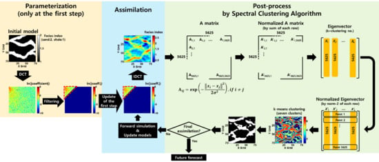
Figure 4 shows an example SCA application example on an average of one hundred updated facies index fields (Figure 4a). An affinity matrix was calculated using Equation (11), and is 5625 by 5625 in dimension because a reservoir grid system is 75 by 75 (Figure 4b). This reflects the relationship between each grid point. This matrix was normalized using the sum of each row (Figure 4c), and the eigenvectors were calculated (Figure 4d). One thing to note is that k, the clustering number, has to be decided in advance. The number of clusters was set to seven in this research based on an experimental sensitivity analysis. According to the experimental analysis, three or four clusters technically worked, but details of facies boundaries needed to be modified. In the case of five or six clusters, the boundary was decent overall. but we put one more cluster for a spare and seven clusters were finally chosen. Although a larger number of clusters than seven can give more details, it requires more computational cost and seven clusters are enough to describe information of facies distribution in this study. In Figure 4e, eigenvectors were normalized using the norm-2 of each row. Then, we regarded each row of the normalized eigenvector as each grid point, which can be assigned to each cluster through k-means clustering, as shown in Figure 4f. In this research, one hundred updated fields were converted into a clustered filed using SCA. Computational cost for application of SCA in the one hundred ensemble members took about nine minutes. The total cost was about 45 min because the number of data assimilations was equal to 5.
Each cluster needed to be determined in sequence of index values so that they could be organized to easily understand which clusters would be sand or shale. In the first place, sand and shale were assigned index numbers 2 and 1, respectively. Naturally, index values of around 2 or 1 will most likely represent sand or shale. Table 1 shows the results of a sequential arrangement. Cluster 6 has the highest average index value. Thus, it is assigned to class A. In contrast, cluster 4 has the lowest average index value, and was assigned to the last class, G.
Figure 5 displays the facies distribution of cluster combinations based on the sequence arrangement and averages of the dynamic data errors. The white indicates sand, and the black is shale. The first row shows each cluster, and the second row indicates the accumulation of each class in sequence such as A, A + B, and A + B + C. For example, the last model in the second row only consists of sand facies due to summation of all clusters. In the last row, a dynamic data error was estimated using Equation (12) to verify which cluster combination is the best to describe a channel pattern.
The combination A + B + C has the lowest error among all of the cluster combinations (the third column) because the main sand facies pattern was grasped out. Therefore, this combination was selected as the best, and we applied an A + B + C combination to one hundred clustered fields using SCA. The facies was assigned as the cluster combination. A reservoir simulation was performed based on this facies distribution.
2.5. Overall Workflow for History Matching
Figure 6 shows the overall workflow of the proposed method, the SCA, for ES-MDA using DCT with one realization example. The entire workflow consists of three parts: parameterization, assimilation, and post-processing. Initial ensemble members were transformed by DCT at the only first step in ES-MDA and DCT coefficients were filtered one realization by one realization (the second column in Figure 1a). The coefficients of each ensemble member were all updated together by the Kalman gain based on ES-MDA. Assimilated DCT coefficients were implemented through an inverse DCT for each realization (the third column in Figure 1a). In the post-processing part, the SCA was applied to the assimilated coefficients of all ensemble members. In this study, the PFR was also tested instead of the SCA for comparison.
One thing of note during the procedure is that the updated reservoir models normally go through parameterization through DCT during every iteration step, as shown in Figure 1a. However, the proposed procedure excluded iterative parameterization of the facies index fields by DCT. It did not move on to the parameterization step after post-processing. Instead of returning to the parameterization phase, it entered the assimilation phase and the DCT coefficients were updated (the far below the assimilation and post-process phases are shown in Figure 6). We can respect the previous updated information of the DCT coefficients, and no artificial modifications occur, thus, information of assimilation can be entirely preserved using ES-MDA.
3. Results and Discussion
In this research, our target was 2D channelized gas reservoirs with an aquifer. The grid size of the reservoir model is 250, 250, and 100 ft for x-, y-, and z-axes, respectively. Reservoir models of the ensemble and the reference field were generated using a single normal equation simulation (SNESim) of the SGeMS. The number of ensemble members was 100. Figure 7a,b shows the training image (TI) used in SNESim and the reference field. The facies proportions of the TI were 28% and 72% for sand and shale, respectively. Figure 8 presents water saturation maps in each time step of observation to understand reservoir behaviors in the reference model. As time goes by, water comes into the reservoir from four sides of the aquifer. It is clear that water behavior absolutely follows the channel. That means figuring out the channel pattern is important for history matching. The sand proportion of the reference is 33%, which was applied to the PFR case. That means the PFR is likely to give a good history matching result, so we can verify the SCA performance strictly through comparison with the PFR.
There were 16 gas production wells. We assumed that there are five observation times until 3500 days with an interval of 700 days. Then, the updated models were simulated from days 0 to 7000 and its prediction was compared with the well behaviors of the reference field. The number of assimilations for history matching was five times. Commercial black oil simulator and Eclipse 100 were used for the forward simulation. An aquifer was developed with pore volume multiplications of four sides of a reservoir model (MULTPV keyword in ECLIPSE). The boundary condition for an aquifer in this study is finite. MULTPV was set about 300 to send a huge amount of water influx to the reservoir. Other reservoir and simulation conditions are described in Table 2.
3.1. Facies Distribution
Before an analysis of the final updated results, we checked how the PFR and SCA work in an updated facies index field. Figure 9 shows three examples of the initial reservoir models, updated facies index, and post-processed results using the PFR and SCA. In the initial models of Figure 9a, facies index fields have values of 2 and 1 for sand and shale, respectively. After updates by ES-MDA such as for the first columns of Figure 9b,c, the models had smeared out channel frontiers and it was hard to tell which area had to be sand or shale. That is the reason why we needed the post-processing techniques of PFR or SCA.
Post-processed results are presented as white (sand) or black (shale) so that updated reservoir models can be simulated with two facies channel model in the forward simulator. In Figure 9b,c, the first column is the updated facies index, which differs due to the different previous assimilated results. In the PFR case, post-processed fields have a clear channel boundary and channel patterns (Figure 9b). In addition, the post-processed fields can provide reliable facies distributions, which are similar to those of the reference field of Figure 7b. This seems to be because the reference sand ratio 33% was applied for the cut-off criterion to classify the facies for PFR. The SCA case shows a better performance than the PFR case in terms of channel connectivity and continuity (Figure 9c). The PFR categorized into sand and shale facies with one specific cut-off. On the other hand, the SCA divided a reservoir model into a couple of areas while considering the spatial distribution of facies parameters. Thus, the post-processed fields using areas divided by the SCA show better geological plausibility of channels. In particular, the second and third post-processed models had improved connectivity in the SCA compared to in the PFR. This verifies that the proposed ES-MDA algorithm coupled with SCA has a good potential to be a trustworthy post-process for an EBM.
Figure 10 shows the initial and final updated facies distribution. In the first row, the sand facies probability maps are presented. They are averages of one hundred realizations. Each value of grid is 0–1, which shows what probability a specific grid has to appear. Figure 10a–c is the initial models and the updated models by PFR and SCA in sequence, respectively. Four reservoir models below the first row are examples among one hundred models of the averages.
Facies probabilities of around 1 indicate a high probability of sand (the red area) and around 0 mean a low probability of sand, and a high probability of shale (the blue area). The drilled well locations are shown as white and blue circles representing sand and shale facies, respectively, as shown in Figure 10a. In the first row of Figure 10a–c, we can infer that there is higher uncertainty in the initial ensemble mean compared to the updated ensemble means by PFR and SCA. In the images, the clear red and blue colors mean that the area most likely to have sand or shale facies. In the initial ensemble mean, the six red spots have a high probability to be sand facies where the drilled positions have sand cores. On the other hand, the yellow and green colored areas between the six red spots have about a 50-50 possibility for sand and shale facies, respectively. It can be said that those colors have qualitatively higher uncertainty. The four initial ensemble members show various channel connectivities of the reservoirs due to limited static data.
The four initial ensemble members show various channel connectivities of the reservoirs due to limited static data. There is potential channel connectivity between every well location in the average of initial models. Therefore, it is important to appropriately break or conserve channel connectivity to figure out a channel pattern of the reference field. Moreover, we should preserve channel properties with geological plausibility. When it comes to this plausibility and channel properties issues, the SCA suggests more suitable updated models than the PFR. In the facies probability maps of Figure 10b,c, an area between well P12 and P15 has a difference of channel connectivity. The SCA result has connectivity. On the other hand, the PFR has broken connectivity between the two wells. The area between the wells is supposed to be linked according to the reference field (Figure 7b). Also, the SCA has overall enhanced connectivity in the four examples of Figure 10b,c. Consequently, the SCA case gives us a stable channel connectivity and pattern compared to the PFR case. The SCA case mimics an S-shaped channel trend, whereas the PFR case does not, although it assumes the best cut-off criterion. These improved channel properties are expected to have a future prediction of the reservoir behaviors.
3.2. Gas and Water Productions
Figure 11 describes the prediction of well gas and water behaviors from 0 to 7000 days of the initial and updated ensemble by the PFR and SCA. Four representative wells with large uncertainty are compared among the sixteen production wells. One of goals of history matching is to properly decrease high uncertainty, which is challenging and necessary at the same time. That is the reason why we need to check uncertainty of reservoir models before and after assimilations. In addition, the sensitivity between reservoir parameters and observations needs to be checked for a successful history matching to calibrate appropriate parameters [40]. The gray lines are the behaviors of one hundred realizations and the blue dotted lines are their means. The red lines are the behaviors of the reference field. The gas production rate is set to be maintain a plateau of 15,000 Mscf/day. In general, gas rates show a plateau until about 2000 days and then they start to go down. The decrease of gas rate is because of mainly two reasons: water breakthrough and pressure decrease. Gas rates of well P1, P9, and P14 decrease with an increase of water rates in the reference model: water breakthrough. On the other hand, gas production rate at well P15 shows a downtrend at around 2500 days without water production. The production rate decreases gradually to maintain the bottomhole pressure at a certain value because bottomhole pressure reaches the constraint of the production well.
Gas production rates of the initial ensemble show a large discrepancy between the blue and red lines, particularly for P14 and P15. The PFR and SCA give well-predicted results in both of the wells. In the PFR case, a couple of grey lines are deviated from the others for wells P9 and P14 (Figure 11b). This seems to be due to a determination of the facies from the cut-off without a consideration of the channel pattern compared to the SCA.
In terms of the well water production rates, they have higher uncertainty than the gas rates because the water behaviors are more sensitive to permeability and an aquifer than the gas behaviors because of the mobility difference. Thus, the water rates from the initial models are affected by the high uncertainty of the facies distribution (Figure 10a) and the uncertainty is represented more noticeably (Figure 10d). In both cases, Figure 11e,f is successful for decreasing uncertainty. The large bandwidths clearly became narrower in P1, P14, and P15. There is connectivity between well P15 and the southern aquifer in some reservoir models out of the initial ensemble members, thus causing a water breakthrough to P15. Water productions of 15 disappear due to updates by the ES-MDA algorithm (P15 of Figure 11e,f). The well P9 was affected by uncertainties of the west aquifer and channel connectivity. These complicated circumstances cause high uncertainty so that the water behaviors of P9 still have large uncertainty, even after assimilations.
Although the PFR case presents decreased uncertainty compared with the initial models, the average and the reference rates are still not matched enough compared to the SCA case. The PFR case is supposed to show fine results because it assumes the best condition for the cut-off criterion. In spite of that, the PFR did not give better results than the SCA. The PFR case did not respect the trend of assimilated values or the channel properties, such as the connectivity and pattern. In contrast, the SCA provided a reasonable prediction of future production with reliable facies connectivity. Besides, the uncertainty from the SCA case is narrower than that of the PFR case. For quantitative analysis of results, Figure 12 shows histograms of the objective functions of the two cases. The objective functions are computed following Equation (13).
where, is the model parameter and is the mean of the prior model. In addition, is the prior model covariance matrix. In Figure 12a,b, the results of an objective function are scaled to 104 for comparison. The average of the objective functions of the PFR case is more than double that of the SCA case. Although the 13 realizations had more than 106 errors in Figure 12a, there were only two realizations in Figure 12b. This explains the reason why the average value of the PFR case is larger than that of the SCA case. From these results, we can verify quantitatively that SCA achieved better history matching performance than the PFR.
4. Conclusions
The proposed method provided new combined auxiliary parameterizations such as DCT and SCA for improvement of ES-MDA performance. SCA works particularly well as a useful post-process to categorize a specific distribution such as a facies distribution and divides it into several territories so that we can recognize an important area as separated parts. In this study, SCA was utilized to help in making a decision about how to assign rock facies into grid-blocks of reservoir models. As in the previous method, PFR is also a post-processing technique to make rock facies indexes discrete. However, the results of PFR are dependent on how index numbers are set for the facies and a cutoff used to categorize facies. Moreover, it is necessary to assume the ratio between rock facies. Even though we determine the true facies proportions (facies ratio of the reference field) in the PFR case, the PFR does not provide geological plausibility and superior results compared to the SCA.
On the other hand, the SCA properly works conserving geological features and plausibility without assumption of the estimated facies proportions or index criterion other than PFR. In addition, SCA decreases the objective functions remarkably compared to the PFR case. The main reason why the SCA achieves a better performance than the PFR is its consideration of the channel trend and overall spatial pattern with the Gaussian affinity. It is also verified that the SCA for ES-MDA coupled with DCT was an appropriate and reliable post-processing method to enhance the history matching performance such as for gas and water well production rates.
Consequently, the SCA can be an alternative to previous post-processing methods because it is satisfactory for facies designation based on quantitative estimation and with respect to geological plausible features at the same time. In spite of those advantages of SCA, there are still three challenges for SCA. Firstly, it needs a standard criterion to decide how many clusters will be proper. Secondly, SCA takes an extra computational cost to calculate the Gaussian affinity. Thirdly, the proposed SCA with DCT and ES-MDA has to be applied to more complicated and practical reservoir models. Although an additional computational time is a limitation of the SCA, this is expected to be mitigated using modified or supplementary calculation methods.
Author Contributions
S.K. wrote programming codes for all of DCT and SCA algorithms and contributed the Introduction, Methodology, and Result. He also summarized the manuscript in the Conclusion Section. K.L. identified the outline of the paper and organized general material of the pictures. Also, he contributed the Abstract and Introduction sections.
Funding
This study is supported by the project of Korea Institute of Geoscience and Mineral Resources (KIGAM) (GP2017-024) and the project of Korea Institute of Energy Technology Evaluation and Planning (KETEP) granted financial resource from the Ministry of Trade, Industry and Energy (MOTIE), Republic of Korea (No. 20172510102090).
Conflicts of Interest
The authors declare no conflict of interest.
References
- Jia, B.; Tsau, J.; Ghahfarokhi, R.B. Investigation of Shale-Gas-Production Behavior: Evaluation of the Effects of Multiple Physics on the Matrix. SPE Reserv. Eval. Eng. 2019. [Google Scholar] [CrossRef]
- Jia, B.; Tsau, J.; Barati, R. A review of the current progress of CO2 injection EOR and carbon storage in shale oil reservoir. Fuel 2019, 236, 404–427. [Google Scholar] [CrossRef]
- Evensen, G. Sequential Data Assimilation with a Nonlinear Quasi-Geostrophic Model Using Monte Carlo Methods to Forecast Error Statistics. J. Geophys. Res. 1994, 99, 10143–10162. [Google Scholar] [CrossRef]
- Nævdal, G.; Manneseth, T.; Vefring, E.H. Near-well Reservoir Monitoring Through Ensemble Kalman Filter. In Proceedings of the SPE/DOE Improved Oil Recovery Symposium, Tulsa, OK, USA, 13–17 April 2002. [Google Scholar] [CrossRef]
- Yeo, M.J.; Jung, S.P.; Choe, J. Covariance matrix localization using drainage area in an ensemble Kalman filter. Energy Sour. Part A Recovery Util. Environ. Eff. 2014, 36, 2154–2165. [Google Scholar] [CrossRef]
- Kim, S.; Lee, C.; Lee, K.; Choe, J. Aquifer characterization of gas reservoirs using Ensemble Kalman filter and covariance localization. J. Pet. Sci. Eng. 2016, 146, 446–456. [Google Scholar] [CrossRef]
- Jung, H.; Jo, H.; Lee, K.; Choe, J. Characterization of various channel fields using an initial ensemble selection scheme and covariance localization. J. Energy Resour. Technol. Trans. ASME 2017, 139, 062906. [Google Scholar] [CrossRef]
- Kang, B.; Yang, H.; Lee, K.; Choe, J. Ensemble Kalman filter with principal component analysis assisted sampling for channelized reservoir characterization. J. Energy Resour. Technol. Trans. ASME 2017, 139, 032907. [Google Scholar] [CrossRef]
- Kang, B.; Choe, J. Regeneration of initial ensembles with facies analysis for efficient history matching. J. Energy Resour. Technol. Trans. ASME 2017, 139, 042903. [Google Scholar] [CrossRef]
- Lee, K.; Jeong, H.; Jung, S.P.; Choe, J. Characterization of Channelized Reservoir Using Ensemble Kalman Filter with Clustered Covariance. Energy Explor. Exploit. 2013, 31, 17–29. [Google Scholar] [CrossRef]
- Park, K.; Choe, J. Use of ensemble Kalman filter to 3-dimensional reservoir characterization during waterflooding. In Proceedings of the SPE Europec/EAGE Annual Conference and Exhibition, Vienna, Austria, 12–5 June 2006. [Google Scholar] [CrossRef]
- Jo, H.; Jung, H.; Ahn, J.; Lee, K.; Choe, J. History matching of channel reservoirs using ensemble Kalman filter with continuous update of channel information. Energy Explor. Exploit. 2017, 35, 3–23. [Google Scholar] [CrossRef]
- Skjervheim, J.A.; Evensen, G. An ensemble smoother for assisted history matching. In Proceedings of the SPE Reservoir Simulation Symposium, The Woodlands, TX, USA, 21–23 February 2011. [Google Scholar] [CrossRef]
- Van Leeuwen, P.J.; Evensen, G. Data assimilation and inverse methods in terms of a probabilistic formulation. Mon. Weather Rev. 1996, 124, 2898–2913. [Google Scholar] [CrossRef]
- Emerick, A.A.; Reynolds, A.C. Ensemble smoother with multiple data assimilations. Comput. Geosci. 2013, 55, 3–15. [Google Scholar] [CrossRef]
- Lee, K.; Lim, J.; Choe, J.; Lee, H.S. Regeneration of channelized reservoirs using history-matched facies-probability map without inverse scheme. J. Pet. Sci. Eng. 2017, 149, 340–350. [Google Scholar] [CrossRef]
- Lee, K.; Jeong, H.; Jung, S.P.; Choe, J. Improvement of Ensemble Smoother with Clustered Covariance for Channelized Reservoirs. Energy Explor. Exploit. 2013, 31, 713–726. [Google Scholar] [CrossRef]
- Lee, K.; Jung, S.; Lee, T.; Choe, J. Use of Clustered Covariance and Selective Measurement Data in Ensemble Smoother for Three-Dimensional Reservoir Characterization. J. Energy Resour. Technol. Trans. ASME 2017, 139, 022905. [Google Scholar] [CrossRef]
- Kang, B.; Lee, K.; Choe, J. Improvement of ensemble smoother with SVD-assisted sampling scheme. J. Pet. Sci. Eng. 2016, 141, 114–124. [Google Scholar] [CrossRef]
- Kang, B.; Choe, J. Initial model selection for efficient history matching of channel reservoirs using Ensemble Smoother. J. Pet. Sci. Eng. 2017, 152, 294–308. [Google Scholar] [CrossRef]
- Emerick, A.A.; Reynolds, A.C. History matching time-lapse seismic data using the ensemble Kalman filter with multiple data assimilations. Comput. Geosci. 2012, 16, 639–659. [Google Scholar] [CrossRef]
- Fan, Z.; Yang, D.; Chai, D.; Li, X. Estimation of relative permeability and capillary pressure for PUNQ-S3 model using a modified iterative ensemble smoother. J. Energy Resour. Technol. Trans. ASME 2018, 141, 022901. [Google Scholar] [CrossRef]
- Evensen, G. Analysis of iterative ensemble smoothers for solving inverse problems. Comput. Geosci. 2018, 22, 885–908. [Google Scholar] [CrossRef]
- Zhao, Y.; Forouzanfar, F.; Reynolds, A.C. History matching of multi-facies channelized reservoirs using ES-MDA with common basis DCT. Comput. Geosci. 2017, 21, 1343–1364. [Google Scholar] [CrossRef]
- Oliver, D.S.; Chen, Y. Recent Progress on Reservoir History Matching: A Review. Comput. Geosci. 2011, 15, 185–221. [Google Scholar] [CrossRef]
- Kim, S.; Lee, C.; Lee, K.; Choe, J. Characterization of channel oil reservoirs with an aquifer using EnKF, DCT, and PFR. Energy Explor. Exploit. 2016, 34, 828–843. [Google Scholar] [CrossRef]
- Kim, S.; Lee, C.; Lee, K.; Choe, J. Characterization of channelized gas reservoirs using ensemble Kalman filter with application of discrete cosine transformation. Energy Explor. Exploit. 2016, 34, 319–336. [Google Scholar] [CrossRef]
- Kim, S.; Jung, H.; Lee, K.; Choe, J. Initial Ensemble Design Scheme for Effective Characterization of Three-Dimensional Channel Gas Reservoirs with an Aquifer. J. Energy Resour. Technol. Trans. ASME 2017, 139, 022911. [Google Scholar] [CrossRef]
- Jung, H.; Jo, H.; Kim, S.; Lee, K.; Choe, J. Recursive update of channel information for reliable history matching of channel reservoirs using EnKF with DCT. J. Pet. Sci. Eng. 2017, 154, 19–37. [Google Scholar] [CrossRef]
- Lorentzen, R.J.; Flornes, K.M.; Nævdal, G. History Matching Channelized Reservoirs Using the Ensemble Kalman Filter. SPE J. 2012, 17, 137–151. [Google Scholar] [CrossRef]
- Lorentzen, R.J.; Nævdal, G.; Shafieirad, A. Estimating Facies Fields by Use of the Ensemble Kalman Filter and Distance Functions-Applied to Shallow-Marine Environments. SPE J. 2013, 3, 146–158. [Google Scholar] [CrossRef]
- Jafarpour, B.; McLaughlin, D.B. History matching with an ensemble Kalman filter and discrete cosine parameterization. Comput. Geosci. 2008, 12, 227–244. [Google Scholar] [CrossRef]
- Jafarpour, B.; McLaughlin, D.B. Reservoir characterization with the discrete cosine transform. SPE J. 2009, 14, 182–201. [Google Scholar] [CrossRef]
- Panwar, A.; Trivedi, J.J.; Nejadi, S. Importance of distributed temperature sensor data for steam assisted gravity drainage reservoir characterization and history matching within ensemble Kalman filter framework. J. Energy Resour. Technol. Trans. ASME 2015, 137, 042902. [Google Scholar] [CrossRef]
- Mouysset, S.; Noailles, J.; Ruiz, D. On an Interpretation of Spectral Clustering Via Heat Equation and Finite Elements Theory. In Proceedings of the World Congress on Engineering 2010, London, UK, 30 June–2 July 2010. [Google Scholar]
- Mouysset, S.; Noailles, J.; Ruiz, D.; Tauber, C. Spectral Clustering: Interpretation and Gaussian Parameter; Springer: Cham, Germany, 2013; Volume 4, pp. 153–162. [Google Scholar]
- Mouysset, S.; Guivarch, R.; Noailles, J.; Ruiz, D. Segmentation of cDNA Microarray Images using Parallel Spectral Clustering. Adv. Distrib. Comput. Artif. Intell. J. 2013, 2, 1–8. [Google Scholar]
- Ahmed, N.; Natarajan, T.; Rao, K.R. Discrete cosine transform. IEEE Trans. Computers 1974, 100, 90–93. [Google Scholar] [CrossRef]
- Kim, S.; Min, B.; Kwon, S.; Chu, M. History Matching of a Channelized Reservoir Using a Serial Denoising Autoencoder Integrated with ES-MDA. Geofluids 2019, 2019, 3280961. [Google Scholar] [CrossRef]
- Yin, Z.; Feng, T.; MacBeth, C. Fast assimilation of frequently acquired 4D seismic data for reservoir history matching. Comput. Geosci. 2019, 128, 30–40. [Google Scholar] [CrossRef]
Figure 1.
(a) One realization example of the discrete cosine transform (DCT) principle and application to history matching procedure and (b) sensitivity analysis of the DCT coefficients.
Figure 1.
(a) One realization example of the discrete cosine transform (DCT) principle and application to history matching procedure and (b) sensitivity analysis of the DCT coefficients.

Figure 2.
One realization example of the preservation of facies ratio (PFR) principle and application to an updated facies index field.
Figure 2.
One realization example of the preservation of facies ratio (PFR) principle and application to an updated facies index field.

Figure 3.
Spectral clustering algorithm (SCA) application for discretization in heat equation.

Figure 4.
SCA application for clustering of an updated facies index field (7 clusters).

Figure 5.
Facies distributions of each cluster and cluster combination with average errors of dynamic data.
Figure 5.
Facies distributions of each cluster and cluster combination with average errors of dynamic data.

Figure 6.
Example of overall update procedures of a channel reservoir using DCT.

Figure 7.
Training image for (a) SNESim and (b) the reference field.

Figure 8.
Water saturation distribution maps of the reference field on the observation time.

Figure 9.
PFR and SCA applications on three reservoir models.

Figure 10.
Comparison between final updated facies distribution using PFR and SCA: Averages of one hundred realizations of (a) initial models, updated models by (b) PFR and (c) SCA in the first row, and four example realizations below the first row.
Figure 10.
Comparison between final updated facies distribution using PFR and SCA: Averages of one hundred realizations of (a) initial models, updated models by (b) PFR and (c) SCA in the first row, and four example realizations below the first row.

Figure 11.
Gas and water well production rates of initial ensemble and updated ensembles using PFR and SCA.
Figure 11.
Gas and water well production rates of initial ensemble and updated ensembles using PFR and SCA.


Figure 12.
Objective functions of one hundred updated ensemble members using PFR and SCA.


Table 1.
Arrangement sequence of clusters based on average index values of each cluster.
| Clusters 1–7 | Average Index Values | Assigned Class |
|---|---|---|
| 6 | 1.9419 | Cluster A |
| 7 | 1.7291 | Cluster B |
| 1 | 1.5202 | Cluster C |
| 3 | 1.3482 | Cluster D |
| 5 | 1.1916 | Cluster E |
| 2 | 1.0533 | Cluster F |
| 4 | 0.9495 | Cluster G |
Table 2.
Simulation and reservoir conditions.
| Parameters | Values |
|---|---|
| Reservoir grid system | 75 by 75 by 1 |
| Well locations, grid coordinate (from the upper left) Well numbering P1–P16 | (14, 14), (30, 14), (46, 14), (62, 14), (14, 30), (30, 30), (46, 30), (62, 30), (14, 46), (30, 46), (46, 46), (62, 46), (14, 62), (30, 62), (46, 62), (62, 62) |
| Observed data types | Well gas production rate, Well bottomhole pressure |
| Porosity, fraction | 0.2 (sandstone), 0.1 (shale) |
| Permeability, md | 100 (sandstone), 1 (shale) |
| Relative permeability, modified Brooks-Corey relation | Connate water saturation = 0.25 Connate gas saturation = 0.2 Sandstone (nw = 3, ng = 2) Shale (nw = 5, ng = 4) |
| Initial water saturation, fraction | 0.25 |
| Initial reservoir pressure, psia | 3000 |
| Bottomhole pressure limit, psia | 1000 |
| The number of DCT coefficients used in a reservoir | 465 (8% of total) |
© 2019 by the authors. Licensee MDPI, Basel, Switzerland. This article is an open access article distributed under the terms and conditions of the Creative Commons Attribution (CC BY) license (http://creativecommons.org/licenses/by/4.0/).
Share and Cite
MDPI and ACS Style
Kim, S.; Lee, K. Application of Spectral Clustering Algorithm to ES-MDA with DCT for History Matching of Gas Channel Reservoirs. Energies 2019, 12, 4394. https://doi.org/10.3390/en12224394
AMA Style
Kim S, Lee K. Application of Spectral Clustering Algorithm to ES-MDA with DCT for History Matching of Gas Channel Reservoirs. Energies. 2019; 12(22):4394. https://doi.org/10.3390/en12224394
Chicago/Turabian StyleKim, Sungil, and Kyungbook Lee. 2019. "Application of Spectral Clustering Algorithm to ES-MDA with DCT for History Matching of Gas Channel Reservoirs" Energies 12, no. 22: 4394. https://doi.org/10.3390/en12224394
Note that from the first issue of 2016, this journal uses article numbers instead of page numbers. See further details here.