Steady-State Power Flow Analysis of Cold-Thermal-Electric Integrated Energy System Based on Unified Power Flow Model

Abstract

The integrated energy system includes various energy forms, complex operation modes and tight coupling links, which bring challenges to its steady-state modeling and steady-state power flow calculation. In order to study the steady-state characteristics of the integrated energy system, the topological structure of the cold-thermal-electric integrated energy system is given firstly. Then, the steady-state model of the power subsystem, the thermal subsystem, the cold subsystem and the distributed energy station are established, the unified power flow model is established, and the Newton Raphson algorithm is used to solve the unified power flow model. Finally, the influence of the key technical parameters on the steady-state power flow of the integrated energy system is analyzed. Research results show that the photovoltaic power generation plays a supporting role in the voltage of each bus; with the increase of electric load power, the unit value of bus voltage decreases continuously; the water supply temperature of the source node has a greater impact on the steady-state flow in the pipeline and the water supply temperature of each node; the pipeline length of the heat network has a greater impact on the end temperature of the pipeline, the water supply temperature, and the return water temperature of each node. The analysis results can support the planning, design, and optimal operation of the integrated energy system.

1. Introduction

Currently, a variety of energy production systems, such as the electric power system, water conservancy system, wind power system, thermal power system, cold energy system, etc., are often operated independently and regulated separately. Each system is lacking in necessary coupling connection and coordinated control, so that the energy utilization rate is low, and energy waste phenomenon is serious. The inefficient energy utilization is hardly in line with the goals of social sustainability and reducing carbon emission [1,2,3]. Therefore, the Energy Internet has been proposed to solve existing problems in energy production, transmission, and utilization [4,5]. The integrated energy system (IES) acts as a basic part of the Energy Internet, and can realize efficient utilization of different energy sources within a region (such as a city, community, industrial park, etc.). IES refers to an integrated system formed by the energy generation, transmission and distribution, conversion, storage, consumption, and other links in the process of planning, construction, and operation [6,7]. It greatly promotes energy consumption and improves the energy efficiency; thus, it has important development prospects and utilization scenarios in the future.

On the basis of system modeling, the simulation analysis of the IES to reveal its operation mechanism and dynamic characteristics is the premise of the application. For the modeling and simulation analysis of the IES, it is necessary to solve the problems of multi-time scale, high dimension, and nonlinearity. A mathematical model of electric power subsystem and natural gas subsystem in IES is established in literature [8]. It presents a global calculation method of multi energy flow of electricity and gas, which can give an accurate solution by using fewer iterations. In reference [9], considering the time and space correlation between load and renewable energy generation, a multi-energy flow calculation method based on nataf transformation and point estimation was proposed. In reference [10], the mathematical model of production, transmission, and consumption links of the IES was established, and the overall mathematical model of the IES was obtained by connecting each link with energy hub. In reference [11], based on the relationship between electricity and heat output of the cogeneration system, different operation modes of the energy hub were analyzed. On this basis, a calculation method of multi-energy flow is proposed, but only the heat load was considered in the paper, and the heat network model was not considered. In reference [12], the mathematical model of the three subsystems of electricity, heat, and gas in the IES was established, the optimal energy flow model was established by selecting appropriate optimization variables, and the intelligent optimization algorithm was used to solve the model. Among the modeling methods of the IES, the concept of the energy hub, proposed by Professor G. Anderson of the Zurich Federal Institute of Technology, has attracted wide attention from academic circles [13,14]. The energy hub highly abstracts and classifies the energy supply and application, which embodies the concept of multi-energy coordination. Although the steady-state modeling of the IES has been carried out in preliminary research at home and abroad, the existing research of the cold-thermal-electric coupling link contains less energy conversion equipment, thus, there is still a lack of practicality in the project. In addition, the accuracy and solving speed of the model still need to be improved.

This article mainly studies the unified power flow of the cold-thermal-electric IES. In Section 2, the electric power subsystem, thermal subsystem, cold subsystem, and the coupling link are modeled to establish a cold-thermal-electric IES model. In Section 3, the unified energy flow model is constructed and Newton-Raphson is used to solve the model. On this basis, Section 5 studies the influence of the key technical parameters on the steady-state power flow of the IES. Finally, the whole paper is summarized in Section 6.

2. Model of Cold-Thermal-Electric IES

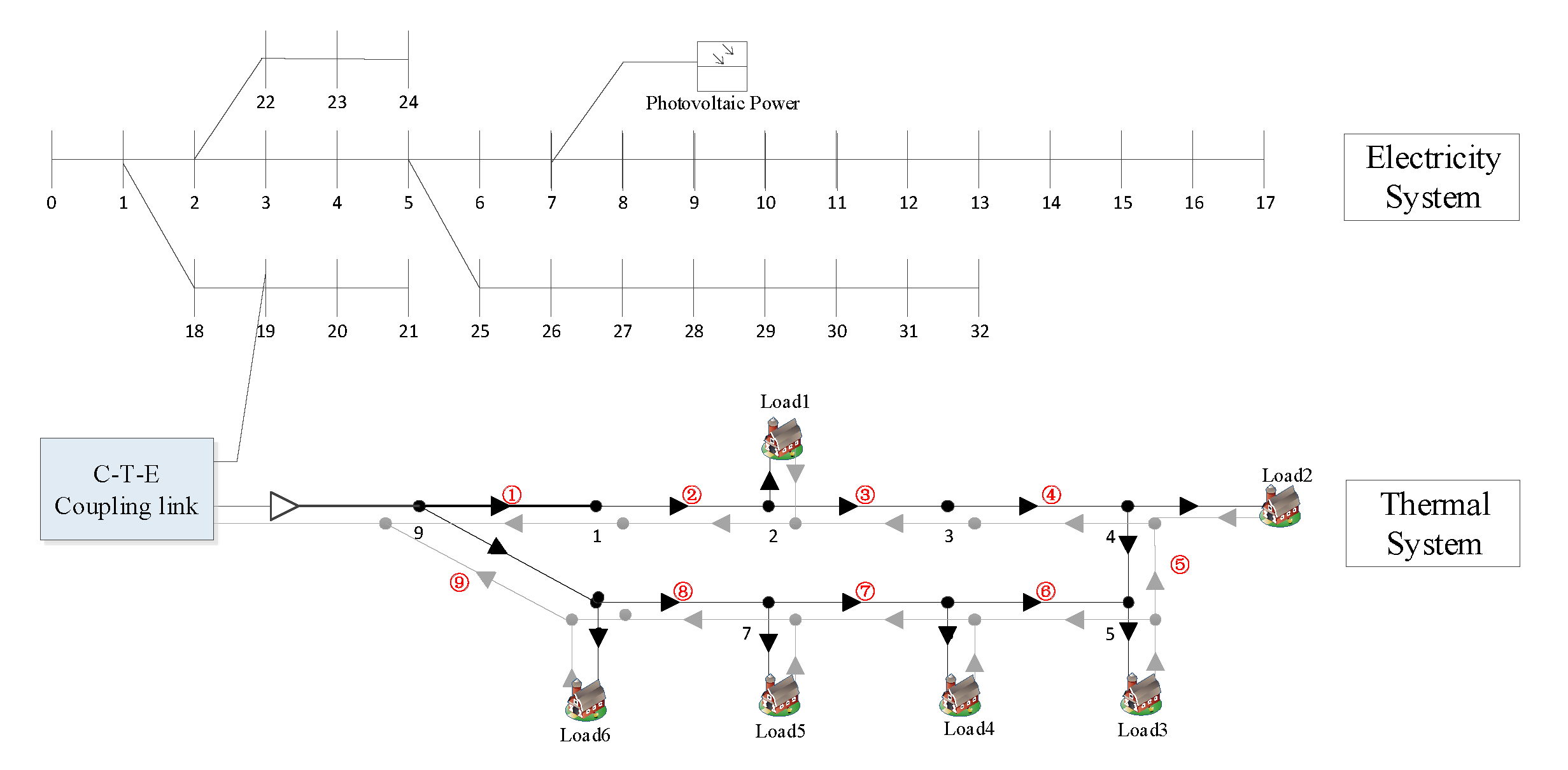
The topology of the cold-thermal-electric IES is shown in Figure 1, which was adopted as the research object in this paper. The 33 node three-phase balance electric power systems [15] and the modified 9 node thermal power system [16] were adopted. The cooling power system is directly connected with the load in order to reduce energy transmission losses.

Thus, the electric power subsystem, thermal subsystem, cooling power subsystem, and coupling link component were modeled in this chapter.

All energy conversion components are modeled in the coupling link, including a combined heat and power (CHP), heat pump (HP), electric boiler (EB) and other electric-thermal coupling components, absorption chiller (AC) and other electric-cooling coupling components, electric chiller (EC) and other electric-cooling coupling components, and an electric power and cooling joint supply (PC) device and other thermal- electric-cooling coupling components.

2.1. Model of Electric Power Subsystem

The traditional model of the power distribution system is adopted for the electric power subsystem. The influence of the three-phase imbalance on power flow calculation is ignored [17]. If the power distribution network has n_e nodes, node1 is the balancing node, node2 to node1 + n_pv are PV node, and the rest of the nodes belong to the PQ node. The model of the power distribution network is the node power equation reflecting the relationship among node power, node voltage and phase angle:

$$P_i=V_i{\displaystyle \sum _{j\in i}{V}_j(G_{ij}\cos {\theta }_{ij}+B_{ij}\sin {\theta }_{ij})}$$

(1)

$$Q_i=V_i{\displaystyle \sum _{j\in i}{V}_j(G_{ij}\sin {\theta }_{ij}-B_{ij}\cos {\theta }_{ij})}$$

(2)

$$P_i=P_{\mathrm{gen},i}-P_{load,i}$$

(3)

$$Q_i=Q_{\mathrm{gen},i}-Q_{load,i}$$

(4)

2.2. Model of Thermal Power Subsystem

Energy is transmitted with water as media in the thermal subsystem, thus, they are modeled by the hydraulic model and thermal power force model.

2.2.1. Hydraulic Model

Based on the graph theory, the characteristics of the pipeline in the thermal subsystem are described, and the flow law in the thermal subsystem is modeled by Kirchhoff’s law for reference. The continuity equation of energy flow can be described by Equation (5):

$$Am=m_q$$

(5)

Head loss is the pressure change per unit length caused by pipeline friction. In a closed circuit, the sum of head losses is zero:

$$B{h}_f=0$$

(6)

where B refers to the loop-pipeline incidence matrix of the thermal subsystem and h_f refers to head loss (m), which can be expressed with Equation (7):

$$h_f=Km\left|m\right|$$

(7)

where K refers to the resistance coefficient of the pipeline.

2.2.2. Thermal Power Model

The solution of the thermal power system is mainly related to the following three temperatures: supply water temperature $T_s$ (the temperature from heat supply network to all thermal load node), outlet water temperature $T_o$ (outlet water temperature of the thermal load node), and return water temperature $T_{\mathrm{r}}$ (the temperature when outlet water of all nodes are mixed into the return water pipeline).

The thermal of all nodes can be expressed as follows:

$$\varphi =C_p{m}_q\left(T_s-T_o\right)$$

(8)

Considering the heat loss of the pipeline, the temperature drop of the water flow at the first and last nodes of the pipeline during its transmission is as follows:

$$T_{end}=\left(T_{start}-T_a\right)e^{-\frac{\lambda L}{C_{p}m}}+T_a$$

(9)

The temperature at the joint of multiple pipes can be calculated according to Equation (10):

$$\left({\displaystyle \sum m_{out}}\right)T_{out}={\displaystyle \sum \left(m_{in}{T}_{in}\right)}$$

(10)

2.3. Model of Cooling Power Subsystem

The model of the cooling power subsystem is similar to that of thermal power subsystem, which also can be described by Equations (5)–(10). No further description is given here.

2.4. Model of Coupling Link

The coupled integrated energy station is adopted for the electricity-thermal-cooling coupling link, the energy conversion and flow relationship is shown in Figure 2.

Energy concentrator theory is adopted for obtaining the following mathematical model of the energy station:

$$\left(\begin{array}{c}{L}_e\\ L_h\\ L_c\end{array}\right)=\left(\begin{array}{c}{c}_{GE,E}+c_{GE,G}{c}_{HP}m\left(1-\mathsf{\alpha }\right)c_{CP,E}\\ c_{GE,H}{c}_{HE,W}+c_{GE,G}{c}_{HP}\left(m\mathsf{\alpha }{c}_{AHP}+\left(1-m\right)\mathsf{\beta }{c}_{LHS}+\left(1-m\right)\left(1-\mathsf{\beta }\right)c_{HE}\right)\\ c_{GE,G}{c}_{HP}m\left(1-\mathsf{\alpha }\right)c_{CP,C}\end{array}\right)\left(P_g\right)$$

(11)

The thermal-to-electric ratio and thermal-to-cooling ratio of the energy station are obtained as follows, under the operation mode of determining electricity/cold through heat:

$$\{\begin{array}{l}{c}_{m,e}=\frac{c_{GE,H}{c}_{HE,W}+c_{GE,G}{c}_{HP}\left(m\mathsf{\alpha }{c}_{AHP}+\left(1-m\right)\mathsf{\beta }{c}_{LHS}+\left(1-m\right)\left(1-\mathsf{\beta }\right)c_{HE}\right)}{c_{GE,E}+c_{GE,G}{c}_{HP}m\left(1-\mathsf{\alpha }\right)c_{CP,E}}\\ c_{m,c}=\frac{c_{GE,H}{c}_{HE,W}+c_{GE,G}{c}_{HP}\left(m\mathsf{\alpha }{c}_{AHP}+\left(1-m\right)\mathsf{\beta }{c}_{LHS}+\left(1-m\right)\left(1-\mathsf{\beta }\right)c_{HE}\right)}{c_{GE,G}{c}_{HP}m\left(1-\mathsf{\alpha }\right)c_{CP,C}}\end{array}$$

(12)

The conversion efficiency of all energy conversion components in the energy station and distribution coefficient of the energy flow are shown in

Table 1. Efficiency of all energy conversion components.

Coefficient	$c_{GE,E}$	$c_{GE,G}$	$c_{GE,H}$	$c_{HP}$	$c_{AHP}$	$c_{HE}$	$c_{LHS}$
Value	0.6	0.1	0.1	3	3	0.98	0.8
Coefficient	$c_{HE,W}$	$c_{CP,C}$	$c_{CP,E}$	$m$	$\alpha$	$\beta$	-
Value	0.98	0.5	0.4	0.9	0.3	0.8	-

.

The thermal-to-electric ratio c_m,e of the energy station is 0.54 through calculation, and the thermal-to-cooling ratio c_m,c is 3.87.

3. Unified Power Flow Model and Calculation Algorithm

Modeling of each decoupling subsystem is the basis of power flow analysis of the IES. It is necessary to set up the system power flow solution model and select the appropriate power flow solution algorithm in order to realize the calculation of power flow of cooling-thermal-electric IES.

3.1. Unified Power Flow Model

The steady-state mixed power flow model of the IES with power subsystem, thermal power subsystem and cooling power subsystem can be expressed through the following form:

$$\{\begin{array}{l}0 = F(x_e,x_h,x_c,x_{eh})\\ 0 = H(x_e,x_h,x_c,x_{eh})\\ 0 = C(x_e,x_h,x_c,x_{eh})\\ 0 = EH(x_e,x_h,x_c,x_{eh})\end{array}$$

(13)

The coupling relationship between above systems can be described by the coupling judgment matrix CO:

$$CO=\left(\begin{array}{ccc}\frac{\partial F}{\partial x_e}& \frac{\partial H}{\partial x_e}& \frac{\partial C}{\partial x_e}\\ \frac{\partial F}{\partial x_h}& \frac{\partial H}{\partial x_h}& \frac{\partial C}{\partial x_h}\\ \frac{\partial F}{\partial x_c}& \frac{\partial H}{\partial x_c}& \frac{\partial C}{\partial x_c}\end{array}\right)$$

(14)

Each element in the equation represents the mutual influence of the energy system. When each element of CO matrix is not equal to zero, the above three energy subsystems are coupled completely; they are dependent on mutual operation state. Coupling mode analysis of the IES is the basis of energy flow analysis. Different mixed power flow solutions should be considered for different coupling modes.

3.2. Solution Algorithm

The theoretical basis for solving the mixed power flow problem lies in that different energy networks all satisfy energy conservation law and material conservation law. However, a large amount of high-dimensional nonlinear equation and decision-making variable are added due to the simultaneous equation of different energy system, which makes the solution of the equations complicated. At present, the Newton-Raphson method is used as a more efficient algorithm for solving the unified power flow model of the IES [16,18].

The essence of power flow calculation is the process of obtaining the system operation point under a given series of conditions for the IES. Since the cooling power subsystem does not have a common node network, modeling of the IES is not conducted for cooling power subsystem. Thus, the unified power flow model of electric-thermal coupling system can be described as follows:

$$F\left(x\right)=\left(\begin{array}{c}\mathsf{\Delta }P\\ \mathsf{\Delta }Q\\ \mathsf{\Delta }\varphi \\ \mathsf{\Delta }p\\ \mathsf{\Delta }{T}_s\\ \mathsf{\Delta }{T}_r\end{array}\right)=\{\begin{array}{l}P-\mathrm{Re}\left\{\dot{U}{\left(Y\dot{U}\right)}^{*}\right\}=0\\ Q-\mathrm{Im}\left\{\dot{U}{\left(Y\dot{U}\right)}^{*}\right\}=0\\ C_p{A}_{s}m(T_s-T_o)-\varphi =0\\ BKm\left|m\right|=0\\ C_s{T}_{s,load}-b_s=0\\ C_r{T}_{r,load}-b_r=0\end{array}$$

(15)

where line 1 and 2, respectively, express the active deviation and reactive deviation of the electric power system, line 3–6, respectively, express node thermal power deviation of the thermal power subsystem, loop pressure drop deviation of the heat supply network, heat supply temperature deviation, and back heating temperature deviation, P, Q, and Φ are, respectively, the active power, reactive power, and thermal power of the system, A_S refers to the reduced order incidence matrix of the heat supply network, C_S and C_r are the matrix, respectively, of the heat supply network and heat supply network structure and flux, B_s and b_r are column vectors related to heat supply temperature and output temperature, respectively, and x = [θ,U,m,T_s,load,T_r,load]^T is the system state quantity.

The unified power flow model is solved through Newton-Raphson Method, and the iteration form is shown as follows:

$$\{\begin{array}{l}\mathsf{\Delta }{x}^{(k+1)}={\left(J^{(k)}\right)}^{-1}\mathsf{\Delta }{F}^{(k)}\\ x^{(k+1)}=x^{(k)}-\mathsf{\Delta }{x}^{(k)}\end{array}$$

(16)

where ΔF refers to the deviation value of the power flow equation set, J refers to Jacobi matrix, x(k) and Δx(k), respectively, refer to the state variable in the k iteration and deviation value of the state variable, and the superscript k represents iterations.

Jacobi matrix J can be expressed as follows:

$$J=\left(\begin{array}{cc}{J}_{ee}& J_{eh}\\ J_{he}& J_{hh}\end{array}\right)$$

(17)

where diagonal block J_ee and J_hh, respectively, refer to the relationship between own power flow of separate electric and thermal systems and own state variable and non-diagonal block J_eh and J_he, respectively, refer to the coupling relationship among the electric and thermal subsystem.

The power flow equation set was solved simultaneously to get the current operation point of the system according to the initial conditions.

4. Example Calculation

The topology shown in Figure 1 and the modeling method in Section 2 were used to establish the unified power flow model for modeling and simulation, and the parameter list of electric power load and thermal power load is given as shown in A1 [19,20] and A2 [17] of Appendix A.

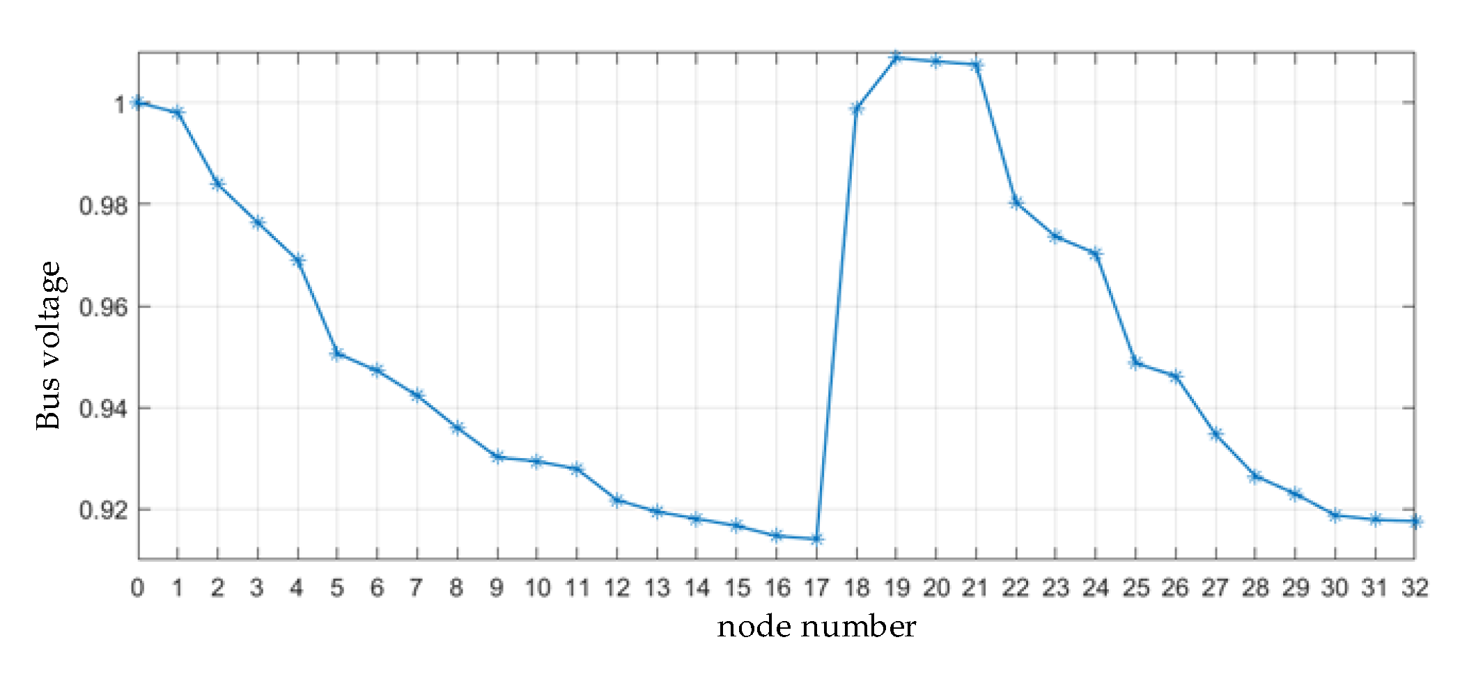
The pipeline flux, node supply water temperature and node return water temperature of the thermal power subsystem are obtained, as shown in Figure 3, Figure 4 and Figure 5, respectively, after alternating iteration operation, and the electric power system bus voltage is shown in Figure 6.

Figure 6 shows that the voltage around power subsystem bus 19 is greatly increased compared, with 33 node power distribution network connected with thermal/cooling network not through the coupling link because the thermal-to-electric ratio of the cooling-thermal-electric coupling link is higher. The coupling link also can provide more electric power at the same time under the condition of meeting the thermal power requirements. Therefore, it has large support role to the electric power system bus voltage.

The load power supplied to the cooling power system is 103.39 kW by calculation through the thermal-to-cooling ratio.

5. Steady State Characteristic Analysis

Due to the close coupling relationship of the integrated energy system, the system model presents the characteristics of multi-input, multi-output, and dynamic change, which causes a change of a certain parameter in the system to directly affect the output characteristics and output state. Thus, it is necessary to carry out a sensitivity analysis and comparison of some parameters of the system. However, it is difficult to analyze the sensitivity change of the whole system, and it is simple and meaningful to analyze the sensitive parameters of a single system. Therefore, this paper will analyze some sensitive parameters of a single system.

5.1. Sensitivity Analysis of Power Subsystem

The sensitive parameters of the electric power subsystem are considered in this section, including the output of photovoltaic power generation. The output of the photovoltaic power generation system is affected by solar radiation intensity, photovoltaic array area, inverter efficiency, and other factors. The maximum output power is shown as follows:

$$P=\epsilon A_{PV}{G}_T\left[1-0.005\left(T_C-25\right)\right]$$

(18)

where ε refers to the photovoltaic conversion efficiency (%) of the photovoltaic array, A_PV refers to the area (m²) of the photovoltaic array, G_T refers to solar radiation intensity (kW/m²), and T_C refers to the solar cell temperature (°C).

Therefore, the output of the photovoltaic power generation is mainly affected by solar radiation intensity G_T. The change group of the solar radiation intensity can be estimated through statistics of previous solar radiation intensity data in the area, thereby obtaining the interval of the photovoltaic power generation output. A group of photovoltaic power generation device is added in bus 7 of the power subsystem as shown in Figure 7.

The value interval of illumination intensity is predicted according to the historical data of illumination intensity, thereby obtaining the output scope of photovoltaic power generation as [119.7, 146.3] kW. Four groups of photovoltaic output data are set as follows: scenario 1 PV output 119.7 kw, scenario 2 PV output 128.57 kw, scenario 3 PV output 137.44 kw, and scenario 4 PV output 146.3 kw. The photovoltaic power generation under four output scenarios is compared with power subsystem flow of the original network not containing photovoltaic (PV) grid connection, which are shown in

Table 2. Power subsystem bus voltage (per unit value) under different PV output scenarios.

Bus No.	Bus Voltage (Per-Unit Value)
	Scenario 1	Scenario 2	Scenario 3	Scenario 4	Excluding PV
0	1.0000	1.0000	1.0000	1.0000	1.0000
1	0.9976	0.9976	0.9976	0.9976	0.998
2	0.9840	0.9840	0.9840	0.9841	0.9839
3	0.9768	0.9768	0.9769	0.9770	0.9764
4	0.9697	0.9698	0.9699	0.9700	0.969
5	0.9520	0.9522	0.9523	0.9524	0.9506
6	0.9487	0.9488	0.9490	0.9491	0.9472
7	0.9444	0.9446	0.9448	0.9450	0.9423
8	0.9382	0.9384	0.9385	0.9387	0.936
9	0.9324	0.9326	0.9328	0.9329	0.9302
10	0.9315	0.9317	0.9319	0.9321	0.9294
11	0.9300	0.9302	0.9304	0.9306	0.9279
12	0.9239	0.9241	0.9243	0.9245	0.9218
13	0.9217	0.9219	0.9221	0.9222	0.9195
14	0.9203	0.9205	0.9206	0.9208	0.9181
15	0.9189	0.9191	0.9193	0.9195	0.9167
16	0.9169	0.9171	0.9173	0.9175	0.9147
17	0.9163	0.9165	0.9167	0.9169	0.9141
18	0.9978	0.9978	0.9978	0.9978	0.9988
19	1.0012	1.0012	1.0012	1.0012	1.0088
20	1.0005	1.0005	1.0005	1.0005	1.0081
21	0.9999	0.9999	0.9999	0.9999	1.0075
22	0.9804	0.9804	0.9805	0.9805	0.9803
23	0.9737	0.9738	0.9738	0.9738	0.9736
24	0.9704	0.9704	0.9705	0.9705	0.9703
25	0.9501	0.9502	0.9504	0.9505	0.9487
26	0.9475	0.9477	0.9478	0.9479	0.9462
27	0.9361	0.9363	0.9364	0.9365	0.9347
28	0.9279	0.9281	0.9282	0.9283	0.9265
29	0.9244	0.9245	0.9247	0.9248	0.923
30	0.9202	0.9204	0.9205	0.9206	0.9188
31	0.9193	0.9195	0.9196	0.9197	0.9179
32	0.9190	0.9192	0.9193	0.9195	0.9176

.

Comparing the data in Table 2, the photovoltaic power generation is regarded as a distributed power supply and connected into the power subsystem. It plays a supporting role to the voltage of all buses, the output is lager, and the supporting role to the bus voltage is larger. Since the capacity of photovoltaic power generation set is smaller, the total power generation capacity can only meet the load demand of bus 7. However, a small part of electric load in bus 7 should be supplied by the power grid. The demand for electric power load of bus 7 is decreased from the perspective of power grid, thus, the voltage of all buses is increased to a small degree, and the voltage at bus 7 drops slowly.

5.2. Sensitivity Analysis of Thermal Power Subsystem

In this section, by adjusting the key technical parameters of the thermal subsystem and solving the steady-state power flow, the influence characteristics of different parameters on the system are analyzed.

5.2.1. Temperature of Source-Node Supply Water

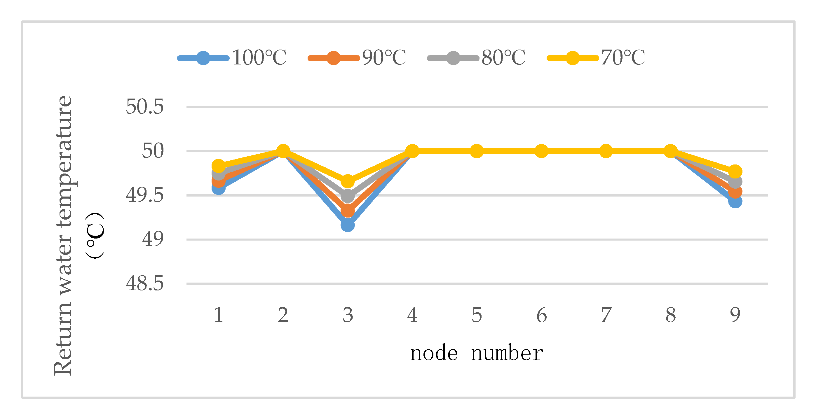
Four groups of different source-node supply water temperatures are set under the condition that the parameters of other technologies are consistent, including: 100 °C, 90 °C, 80 °C, and 70 °C. The steady-state power flow under different source-node supply water temperatures was calculated. The pipeline steady-state flux, node supply water temperature and node return water temperature were obtained, as shown in the Figure 8, Figure 9 and Figure 10.

Figure 10 shows that the source-node supply water temperature is lower and the steady-state flux in the pipeline is higher. The same conclusion also can be obtained by the thermal equation:

$$\varphi =C_p{m}_q\left(T_s-T_o\right)$$

(19)

When the load thermal power Φ is constant and the node outlet water temperature T₀ is the same, the node supply water temperature T_s is lower, the flux m_q for the load is larger, and the pipeline flux in the heat supply network system is also larger. Figure 8 shows that the supply water temperature of all nodes is also reduced when the source-node supply water temperature is reduced. However, the relative relationship among all node supply water temperatures remains unchanged. Figure 9 shows that the return water temperature of all load nodes is still the same, with the set outlet water temperature under different source-node supply water temperatures, namely 50 °C. The return water temperature of the non-load node is slightly increased with the increase of the source-node supply water temperature, and the change trend is small.

Parameter changes of the thermal power subsystem have influence on the electric power subsystem through the coupling link. Since the thermal power subsystem scale is much smaller than the power subsystem, the source node supply water temperature changes in the thermal subsystem may generate almost no influence on the electric power subsystem. For example, it can be seen that when the water supply temperature of the source-node of the thermal subsystem changes, the steady flow of the pipeline and the return water temperature of the node have a great influence, but have little effect on the power subsystem. The output of the power subsystem and the cold subsystem cannot be changed under the operation mode of determining electricity with heat or determining cold with heat.

5.2.2. Pipeline Length of Heat Supply Network

All technical parameters were consistent, taking the parameters of the example in Section 4 as the standard, and with four groups of different pipe lengths of the heat supply network: 0.5 times standard length, 0.75 times standard length, standard length, and 1.25 times standard length. The steady-state power flow under different pipeline lengths of the heat supply network was calculated. Steady-state pipeline flux, node supply water temperature and node return water temperature were obtained, as can be seen in Figure 11, Figure 12 and Figure 13.

It can be seen from Figure 11, Figure 12 and Figure 13 that when the pipe length of the heat supply network increases, the steady-state pipe flow increases by a small margin, and the supply water temperature and the return water temperature of each node decrease by a small margin. This is because with the increase of the pipe length of the heating network, the loss of heat in the transmission process with water as the medium increases, which is shown as the increase of temperature loss, as shown in the drop formula of water flow temperature at the first and last nodes of the pipe:

$$T_{end}=\left(T_{start}-T_a\right)e^{-\frac{\lambda L}{C_{p}m}}+T_a$$

(20)

The pipeline length L is larger, the temperature of the pipeline terminal is lower. Therefore, both supply water temperature and return water temperature of all nodes are decreased, and the supply water temperature is decreased more obviously. Therefore, the temperature difference of the thermal power supplied by the thermal-supply pipe network is decreased, and the pipeline flux is increased accordingly, thereby ensuring adequate supply of thermal load.

The changes of the heat supply network pipeline length in the thermal power subsystem may produce certain influence on steady-state pipeline flux in the thermal power subsystem as well as node supply water temperature and return water temperature. There is almost no influence on the power subsystem and cooling power subsystem.

6. Summary

In this paper, the hybrid power flow model of the cold-thermal-electric IES is established, in which the cold-thermal-electric coupling link is modeled based on the energy hub, and the hybrid modeling of the IES is realized. On this basis, the Newton Raphson algorithm is used to decompose the hybrid power flow. The steady-state characteristics of the IES are obtained, and the influence characteristics of the key technical parameters of the power subsystem and the thermal subsystem on the steady-state tide flow of the IES are discussed

• After photovoltaic power generation is incorporated into the power subsystem as a distributed power source, it plays a supporting role for each bus voltage, and the larger the output, the greater the supporting role for the bus voltage.
• With the increase of electric load power, the unit value of bus voltage is decreasing, that is, the voltage loss is increasing. At this time, the role of the distributed generation is particularly important, thus, it is necessary to study the steady-state power flow considering the interaction of the distributed generation and the load fluctuation.
• The lower the source-node water supply temperature, the higher the steady-state flow in the pipeline, and the lower the node water supply temperature. However, the return water temperature of each load node is still the same as the set outlet water temperature. The return water temperature of the non-load node rises slightly with the decrease of the water supply temperature of the source node, with little change.
• When the pipe length of the heating network increases, the steady flow of the pipe increases by a small margin, the water supply temperature and return water temperature of each node decrease by a small margin, and the end temperature of the pipe decreases; thus, the water supply temperature and return water temperature of each node decrease.

The results can support the planning, design and optimal operation of the integrated energy system.

References

- Yang, Y.; Fang, Z.; Zeng, F.; Liu, P. Research and Prospect of Virtual Microgrids Based on Energy Internet; IEEE: Piscataway, NJ, USA, 2017; pp. 1–5. [Google Scholar]
- Holmes, J. A More Perfect Union: Energy Systems Integration Studies from Europe. IEEE Power Energy Mag. 2013, 11, 36–45. [Google Scholar] [CrossRef]
- Sun, H.; Guo, Q.; Zhang, B.; Wu, W.; Wang, B.; Shen, X.; Wang, J. Integrated Energy Management System: Concept, Design, and Demonstration in China. IEEE Electrif. Mag. 2018, 6, 42–50. [Google Scholar] [CrossRef]
- Ma, T.; Wu, J.; Hao, L.; Yan, H.; Li, D. A Real-Time Pricing Scheme for Energy Management in Integrated Energy Systems: A Stackelberg Game Approach. Energies 2018, 10, 2858. [Google Scholar] [CrossRef]
- Qian, A.; Ran, H. Key Technologies and Challenges for Multi-energy Complementarity and Optimization of Integrated Energy System. Autom. Electr. Power Syst. 2018, 42, 1–8. [Google Scholar]
- Jia, H.; Wang, D.; Xu, X.; Yu, X. Research on Some Key Problems Related to Integrated Enery System. Autom. Electr. Power Syst. 2015, 39, 198–207. [Google Scholar]
- Cheng, H.; Hu, X.; Wang, L.; Liu, Y.; Yu, Q. Review on Research of Regional Integrated Energy System Planning. Autom. Electr. Power Syst. 2019, 43, 2–13. [Google Scholar]
- Martinez-Mares, A.; Fuerte-Esquivel, C.R. A unified gas and power flow analysis in natural gas and electricity coupled networks. IEEE Trans. Power Syst. 2012, 27, 2156–2166. [Google Scholar] [CrossRef]
- Sun, G.; Chen, S.; Wei, Z.; Li, Y. Probabilistic Optimal Power Flow of Combined Natural Gas and Electric System Considering Correlation. Autom. Electr. Power Syst. 2015, 39, 11–17. [Google Scholar]
- Krause, T.; Andersson, G.; Frohlich, K.; Vaccaro, A. Multiple-energy carriers: Modeling of production, delivery, and consumption. Proc. IEEE 2011, 99, 15–27. [Google Scholar] [CrossRef]
- Xu, X.; Jia, H.; Jin, X.; Yu, X.; Mu, Y. Study on Hybrid Heat-Gas-Power Flow Algorithm for Integrated Community Energy System. Proc. CSEE 2015, 35, 3634–3642. [Google Scholar]
- Shabanpour-Haghighi, A.; Seifi, A.R. Simultaneous integrated optimal energy flow of electricity, gas, and heat. Energy Convers. Manag. 2015, 101, 579–591. [Google Scholar] [CrossRef]
- Sun, H.; Pan, Z.; Guo, Q. Energy Management for Multi-energy Flow: Challenges and Prospects. Autom. Electr. Power Syst. 2016, 40, 1–8. [Google Scholar]
- Wu, J. Drivers and State-of-the-art of Integrated Energy Systems in Europe. Autom. Electr. Power Syst. 2016, 40, 1–7. [Google Scholar]
- Han, L. Interval-Affine Analysis Method in Power System with Consideration of Intermittent. Ph.D. Thesis, Tianjing University, Tianjin, China, 2014. [Google Scholar]
- Liu, X.; Jenkins, N.; Wu, J.; Bagdanavicius, A. Combined Analysis of Electricity and Heat Networks. Energy Procedia 2014, 61, 155–159. [Google Scholar] [CrossRef]
- Pan, Z.; Guo, Q.; Sun, H. Interactions of district electricity and heating systems considering time-scale characteristics based on quasi-steady multi-energy flow. Appl. Energy 2016, 167, 230–243. [Google Scholar] [CrossRef]
- Luo, B.; Mu, Y.; Zhao, B. Static Sensitivity Analysis of Integrated Electricity and Gas System Based on Unified Power Flow Model. Autom. Electr. Power Syst. 2018, 42, 29–35. [Google Scholar]
- Wang, W.; Wang, D.; Jia, H.; Chen, Z.; Guo, B.; Zhou, H.; Fan, M. Review of Steady-state Analysis of Typical Regional Integrated Energy System Under the Background of Energy Internet. Proc. CSEE 2016, 36, 3292–3306. [Google Scholar]
- Wang, Y.; Zeng, B.; Guo, J.; Shi, J.Q.; Zhang, J.H. Multi-Energy Flow Calculation Method for Integrated Energy System Containing Electricity, Heat and Gas. Power Syst. Technol. 2016, 40, 2942–2951. [Google Scholar]
Figure 1.
Topology of cooling-thermal-electric integrated energy system.
Figure 2.
Energy flow chart of cooling-thermal-electric coupling link.
Figure 3.
Pipeline flux of thermal power subsystem.
Figure 4.
Node supply water temperature of thermal power subsystem.
Figure 5.
Node return water temperature of thermal power subsystem.
Figure 6.
Bus voltage of power subsystem.
Figure 7.
IES containing photovoltaic power generation in bus 7.
Figure 8.
Pipeline flux under different source-node supply water temperatures.
Figure 9.
Supply water temperature of all nodes under different source-node supply water temperatures.
Figure 10.
Return water temperature of all nodes under different source-node supply water temperatures.
Figure 11.
Pipeline flux under different pipeline lengths.
Figure 12.
Supply water temperature of all nodes under different pipeline lengths.
Figure 13.
Return water temperature of all nodes under different pipeline lengths.