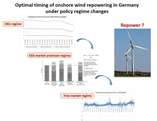
Optimal Timing of Onshore Wind Repowering in Germany under Policy Regime Changes: A Real Options Analysis


1
Institute for Future Energy Consumer Needs and Behavior (FCN), School of Business and Economics/E.ON Energy Research Center, RWTH Aachen University, Mathieustraße 10, 52074 Aachen, Germany
2
Department of Industrial Economics and Technology Management, Norwegian University of Science and Technology (NTNU), 7491 Trondheim, Norway
3
RWTH Aachen University, Templergraben 55, 52056 Aachen, Germany
*
Author to whom correspondence should be addressed.
Energies 2019, 12(24), 4703; https://doi.org/10.3390/en12244703
Submission received: 31 August 2019
/
Revised: 5 December 2019
/
Accepted: 6 December 2019
/
Published: 10 December 2019
(This article belongs to the Special Issue Economics of Sustainable and Renewable Energy Systems)
Abstract
:In this paper, we investigate capacity expansion, the technological development of wind turbine generators, and the merits of onshore wind repowering in Germany. We analyze the regulatory framework that is presently in place and its impact on the profitability of the onshore wind parks commissioned under previous regulatory frameworks. The optimal timing of repowering under today’s market premium model is scrutinized. Repowering in a market without subsidies for onshore wind energy is also evaluated. In the two cases (regimes) investigated, the electricity price is modeled stochastically as a geometric Brownian motion process. More specifically, using a real options modeling framework for investments under a free market regime, we analyze how the regime change affects the optimal timing of repowering. Further, we check the results for their robustness via a sensitivity analysis for both analyzed regimes. We find that repowering well before the plant’s expected end of life (‘early repowering’) can be economically preferable under the German Renewable Energy Sources Act 2017 remuneration scheme and that, due to the electricity spot market price development, repowering under the market premium regime is more profitable than it is under the free market regime. The economic viability is strongly influenced by the duration of the initial tariff granted to the old installation, the expected digression factor of the future reference tariff, and the increase in electricity generation achieved through repowering.
1. Introduction
The European Commission passed indicative climate and energy targets for member countries for the first time in 2001 [1]. Since then, the capacity of renewable energy sources (RES) has increased rapidly in the EU. This growth can mainly be attributed to the implementation of policy measures on a national level in order to attract investments in this sector. Especially onshore wind capacity has been deployed extensively, because it is one of the low-cost renewable energy technologies (RET) in most countries [2] (and it plays a significant role in today’s electricity generation. As the expansion of onshore wind started in some countries already in the late 1970s, the best wind sites are nowadays often engaged by less efficient, relatively small-scale wind turbine generators (WTGs); also, land constraints for greenfield developments are faced. With an increasing number of old turbines reaching at least the second half of their service lifetime, repowering is in many cases becoming an economic opportunity. In the context of our analysis, repowering refers to the replacement of old WTGs by new ones, in contrast to developing a greenfield project. This carries inter alia the possibility for further net capacity additions and often yields a significant increase in renewable electricity generation, which can contribute substantially to reaching national and EU targets.
The investment conditions set by national policy frameworks are essential for onshore wind repowering to be economically feasible and, in general, for further RES additions. As policy schemes are not only under constant revision by national legislators, but also by the EU Commission, they can change quite frequently. The latter recently passed the “Guidelines on state aid for environmental protection and energy 2014–2020”, which oblige member states to implement more market-oriented RES incentive schemes.
The focus of our study is Germany as one of the pioneer countries for wind power and the largest onshore wind market in Europe. The main original contribution of this study is two-fold: (1) the analysis of how the changes in the regulatory framework impact the profitability of the existing wind power plants and repowering decisions; (2) an analysis of the impact of applying a dividend yield to the underlying project on the threshold value and probability of repowering. Section 2 provides a concise overview of related literature using real options analysis in the context of RET investment under different regimes, and repowering in particular. In Section 3, an overview of the onshore wind power market development in Germany is provided, including capacity additions, technological development of WTGs, and the merits of repowering. In Section 4, the various amendments of the German Renewable Energy Sources Act (Erneuerbare Energien Gesetz—EEG) and the current regulatory framework are briefly described, paving the way for economic analysis of the effect of different frameworks on the timing of repowering, which in this form is novel. Further, the regulatory regimes are evaluated with regard to the uncertainty inherent in the revenue stream of the new onshore wind asset, as described in Section 5. The two settings analyzed are the market premium model and the free market regime without any subsidies in order to show the effect of market exposure. In Section 6, the models derived for the three scenarios are applied to a fictional wind park and the results obtained are discussed. Section 7 concludes and provides some ideas for further research.
2. Related Literature
In real options analysis (ROA) the value of a firm does not only depend on the present value of assets in place, but also on the present value of future growth options. As the latter cannot be determined by classical investment calculation, the principles of financial options theory are applied to real assets. ROA has become increasingly popular and the spectrum of topics covered by ROA in the power sector is manifold. While in this paper only revenue uncertainty is taken into consideration, along with the analysis of other deterministic factors that can have an impact on the repowering decision, the following literature has treated investments in RET under different aspects. Murto [3] analyzed the effect of uncertainty in revenues and technology. He finds that technological uncertainty has no effect on the optimal investment policy, while it decreases the attractiveness of an investment when combined with revenue uncertainty. The effect of learning curve information on the diffusion of RET is analyzed within a dynamic programming model by Kumbaroğlu et al. [4], taking the increasingly deregulated market of Turkey as an example. The authors find that due to the high cost of RES, additional support to that of the renewable energy law in place at the time, is needed to attract investments in RET, especially in a liberalized market. Rohlfs and Madlener [5] compare investments in different power generation technologies, taking into account multiple underlying, technology-specific prices, such as those of fuel, CO2, and electricity. Due to the correlation of the underlying variables the optimal investment strategy for the erection of generation units is investor-dependent. Among other findings, the increase of the expected net present value (NPV), the value of waiting, and the asymmetric distribution of the cash flows is shown. Heggedal et al. [6] analyze the effect of policy uncertainty on investments in small hydropower plants in Norway. They observe a greater delay of investments among professional investors than among non-professionals. They find that there was strong evidence of non-professionals assuming a “now-or-never” perspective, while professional investors tend to compare immediate investment with the value of continuing to wait for clarification in the discussion over policy support. Research on the comparison of support mechanisms was, among others, performed by Boomsma et al. [7], who study the capacity choice and investment timing under a feed-in tariff (FIT) and green certificate trading. In a case study for an onshore wind park in Norway, they find that investments are taken earlier under an FIT regime, whereas larger projects are realized under certificate trading. Concerning repowering, Madlener and Schumacher [8] examine the risk and potential of repowering in Germany with simulations, whereas Himpler and Madlener [9] use ROA for the analysis of repowering in Denmark, considering investment and revenue uncertainties. Ritzenhofen and Spinler [10] assess investment behavior with respect to onshore wind farms under a FIT regime and a free market regime, and the effect of a regime switch. The authors find inter alia that under a sufficiently attractive FIT regime, future regime changes have little impact on current investment projects as they represent now-or-never decisions. Kitzing et al. [11] analyze wind power project investments under different support schemes (feed-in tariffs, feed-in premia and tradable green certificates) using an ROA applied to offshore wind in the Baltic Sea. In the optimization, the authors impose a capacity constraint and explore the trade-off between faster (slower) deployment of smaller (larger) projects. Anatolitis and Welisch [12] develop an agent-based model of onhore wind power auctions (uniform and pay-as-bid pricing) for Germany. They find lower prices for pay-as-bid auctions (but at the expense of lower allocative efficiency of that type of auction) and identify threats to smaller operators and their diversity in the longer run, learning the effects of lowering the strike price. Voss and Madlener [13] analyze different auction schemes, bidding strategies, and the cost-optimal level of promoting renewable electricity in Germany. Moon and Baran [14] apply ROA for determining the optimal time to invest in a (small or large) residential photovoltaic system, and the differences in project deferral for the cases of Germany, Japan, Korea, and the US. Gazheli and van den Bergh [15] investigate a community’s optimal investment strategy in solar PV or wind power using an ROA approach. They assume uncertainty in electricity prices and the speed at which learning drives down technology costs and study its impact on the threshold to investment. Finally, Ruberg et al. [16] propose a levelized cost of electricity (LCOE)-based decision support tool aimed to assist with lifetime extension decisions for onshore wind turbines. As part of a case study, the tool is applied to a wind park in the UK that comprises six 900 kW turbines.
3. Wind Energy and Repowering in Germany
The German Energiewende (sustainable energy transition) stipulates that the share of RES in final energy consumption should reach 18% by 2020, 30% by 2030, and 45% by 2040. The target share of RES in gross electricity consumption is 40–45% in 2025 and 55–60% in 2035 [17]. As one of the least-cost RETs, onshore wind plays a key role in reaching this target and has experienced significant capacity additions since the introduction of the EEG in 2000 (see Appendix A.1 for details). In 2018, the production of RES-E reached 546 TWh (40.6%) of gross electricity consumption. Wind power contributed around 112 TWh (20%), making it the largest source of renewable electricity ahead of the 45 TWh (8.2%) from biomass [18].
3.1. Installed Onshore Wind Capacity and Technological Development
The annual capacity additions of onshore wind in Germany already started to pick up speed around 1996, and experienced a significant increase in 2000, when the EEG was introduced. Since then, the yearly additions have never fallen below 1.4 GW and reached a record high in 2017 of 5.3 GW (Figure 1). The high volatility in the capacity additions can partly be explained by developers rushing to finish (or delaying) their projects, when amendments of the EEG were about to be passed that either lowered or raised the amount of remuneration, respectively. It would explain the drop of installed capacity in 2018, after the adoption of the EEG 2017. The increasing resistance among the population to new wind turbines (WT) and increasing prices of raw materials were two main factors explaining the decrease in annual capacity additions after 2002 [8] (p. 298). Figure 1 also shows the effect of varying wind conditions on the electricity production. For example, between 2008 and 2010, the wind power production output experienced a significant drop due to comparatively poor wind conditions even though the installed capacity increased by over 4.5 GW.
The use of wind power naturally started in the north of Germany (i.e., Lower Saxony, Schleswig-Holstein, Mecklenburg-Western Pomerania, Bremen, and Hamburg), close to the shoreline, due to better wind conditions than in central or southern Germany. Since the technology was still in its infancy twenty-five years ago, the average WTG deployed in 1995 had only a hub height of about 45 m, a rotor diameter of 40 m, and a capacity of 500 kW. As the turbines were so small by today’s standards, many had to be deployed to achieve the capacity additions shown in Figure 1, so that by the end of 2013 around 1300 WTGs had already reached or exceeded their assumed 20 years of service life. This number represents about 5.5% of all installed WTGs, but only 0.68% of the total nominal power.
Figure 2 depicts the age structure of the wind turbines by size class in Germany. Note that the nominal capacity reported does not correspond exactly with the capacity in Figure 1, because the underlying data used by [22] lists only WTs that have been registered by the owner, the operator, or the original equipment manufacturer. Therefore, this database does not claim completeness, but it is a very good indicator which has been used by many professional researchers.
Due to the quick increase in the size of WTGs (‘upscaling’), land constraints in the north of Germany, and because the EEG linked the remuneration for electricity from WTGs to the quality of the wind site (see Appendix A), the attractiveness of projects on lower quality wind sites increased. More capacity additions could be observed in central and southern Germany and, since 2004, the percentage of the capacity added in the north has stabilized at around 45%.
In 2018, the average installed WT had a capacity of 3.34 MW, a hub height of 133 m, and a rotor diameter of 118 m, reflecting the remarkable increase in size since 1995 (Figure 3). With the market share of the 3–4 MW turbine class reaching 70% and manufacturers testing even larger prototypes, further increases in average size can be expected. As many as 114 different designs of WTGs were deployed, increasingly adapting to the conditions of a specific site by the choice of rotor diameter and hub height. The rotor diameter hereby varies between 48 m and 149 m, the latter being the one of a Nordex N149 [24]. This increase in size and capacity, as well as technological developments are reasons why repowering is becoming an attractive opportunity at the end of a WTG’s service life. Therefore, it is discussed in more detail in the following.
3.2. Purpose and Effects of Repowering
In short, onshore wind repowering means the process of decommissioning old WTs and replacing them with new, more energy-efficient WTs either on the same site or close to it. In Germany, the new WTG needed to be in the same or adjacent rural district to be subject to the repowering remuneration paid under former EEG versions (for details, see Section 5). According to [25] (p. 11), five alternatives for repowering exist: (1) 1:1 upscaling of single wind turbines (a case rather uncommon in Germany, since building permits are not granted for constructing single WTs); (2) 2:1 replacement: two smaller, old WTs are replaced by one larger, new WTG; (3) Clustering of single WTGs into wind farms; (4) 1:1 replacement of WTGs with similar rates, but newer machinery, and (5) 1:1 upscaling of wind farms (in Germany, this is usually difficult to achieve, because of the increase in demand for space of the larger new WTGs).
Repowering has come into the focus of many developers and asset owners, since land constraints are faced, especially in regions of prime wind classes, where numerous first-generation WTs are deployed, and an increasing number of assets are reaching the end of their service life. Due to the enormous increase in productivity of new WTs, repowering can also be the preferred choice many years before the end of the service lifetime is reached, and this is referred to as “early repowering”.
The drivers for repowering are numerous and can be divided into two categories. The drivers shared with greenfield projects, e.g., federal goals for RES, and the drivers specific to repowering. The following list of drivers provides an overview of the latter, without claiming completeness.
- ○
- Higher capacity, production, and efficiency. As seen in Figure 3, there has been an enormous increase in the size and capacity of WTs over the last years, which results in a higher production output. Furthermore, the growth in rotor diameter, improvements in aerodynamics, etc. have led to a much higher availability over a wider range of wind speeds. The example of a repowering project in Galmsbüll (in the federal state of Schleswig-Holstein) illustrates this increase in productivity and the decrease in the number of turbines (see Table 1).
- ○
- O&M costs. According to [27] (p. 1), the operational costs of WTs may increase by 25% after 10 years of operation; LIE [20] (p. 53) also states an increase of 20% in the second half of a WT’s lifetime, which can make repowering attractive. The O&M costs per MWh for new WTs can be expected to be lower than those for old ones, which may be due to the fact that recent projects have used larger turbines with a higher capacity factor ([28]; on the capacity factor see also Section 5.1). The newer machinery also reduces downtimes, since it is less likely to fail.
- ○
- Load factor. Hughes [29] (p. 7) found that the normalized load factors for onshore wind farms in Denmark declined from a peak of 22% at age zero to 18% at age 15 (24% to 11% in the UK). This results in a tremendous decrease in electricity production. The effect on the timing of repowering involved in such a decline is quantified in Section 6.
- ○
- ○
- Grid integration. New WTGs not only produce electricity more steadily (see above), but can also provide grid services, since their maximum active power needs to be remotely controllable by the transmission system operator (TSO), thus supporting grid stability. Also, as discussed in Section 4, regional grid capacity limitations and the rapid expansion of wind power installations may compromise grid stability. Repowering, if properly incentivized, can help to mitigate locational inefficiencies of RES generation and the need for RES curtailments [31].
- ○
- Reduction in the number of WTGs and bundling. Repowering usually helps to significantly decrease the number of installed WTs, while an increase in capacity and production is achieved. Additionally, it offers the opportunity to decommission scattered WTs and to bundle them in designated areas. This allows for the correction of any mistakes that were made in the regional and land-use planning [32]. On top of that, today’s WTs turn more slowly than old ones, which can also help to reduce the visual impact on the surroundings.
- ○
- Tax benefits. Since the trade tax law of 2009 came into effect, the municipalities where WTs are commissioned receive at least 70% of the trade tax yield, the municipality of the asset operator only 30% [33] (Art. 29). Turning local residents into stakeholders of a wind park can additionally increase the acceptance of projects through monetary incentives.
- ○
- Financial risks. The risk of a repowering project might be lower than that of a greenfield development, as good wind data are already available, improving the production forecast accuracy of electricity, thus making it easier to get favorable loan terms and allowing a very high gearing with sometimes less than 10% equity [30]. Also, contact with local communities has already been established [8] and the integration into the planning process might be easier.
- ○
- Availability of favorable sites. As mentioned above, repowering is becoming especially attractive when favorable wind sites are already occupied by old WTGs, and when available sites are scarce.
- ○
- New permitting process. Old WTs have usually been built under different regulatory and environmental frameworks and also, due to the increase in the size of WTs, the permit process can be considered to be as difficult as that of a greenfield project [30]. In contrast, resistance from local communities can often be expected, because of the height of new generation WTs and their visibility from a great distance, especially at night, since constructions higher than 100 m have to be marked with beacons.
Figure 4 shows that repowering has gained momentum in the recent past and that WTGs commissioned under repowering projects made up for over 25% of the total added capacity in 2013. Whereas in the past, repowering was promoted by the EEG, since August 2014 the dismantling of wind turbines has only been carried out on the basis of the condition of the plant or because the site can be used more profitably with a modern wind turbine. This legislative change resulted in a decline in repowering projects (cf. Figure 4). From 1252 installed WTGs in 2015, only 226 WTGs were installed within the framework of repowering [34].
However, the theoretical potential for further repowering projects in the near future is still large, and repowered projects might still make up for a significant share of the future annual capacity additions, even though financial subsidies were abolished in 2014. One indicator is the number of WTs installed and their capacity before 2002, because under the EEG 2012 a repowering bonus was paid if the decommissioned WTGs were deployed before 2002, indicating economic feasibility. Furthermore, these WTGs have already reached the second half of their service life today. According to [20], 10,400 WTs fell under this category, totaling a capacity of 8250 MW. This is equivalent to 43% of all WTGs, but only 25% of the installed capacity. Obviously, most of them are located in the northern parts of Germany (Figure 5). Therefore, the spatial-temporal diffusion of repowering will likely be similar to the general development of wind power and concentrate at first in the north.
The numbers mentioned previously are only a theoretical value for the potential of repowering, though, since height restrictions and distance regulations in some rural districts may reduce this potential. Additionally, planning and building regulations limit areas where WTs can be commissioned (for an overview of the latter, including their significance for repowering projects, see, e.g., [8]).
4. Policy Frameworks in Germany from 1991 Until Today
Since, in most cases, RES-E has been more expensive than electricity from conventional generation and has still not reached grid parity in most countries yet, incentives are to be introduced to promote the use of RET. Therefore, the German government passed the Electricity Feed-In Law (Stromeinspeisungsgesetz, StrEG) in 1991. This was the first law subsidizing RES-E in Germany, superseded in 2000 by the EEG (Erneuerbare Energien Gesetz), which has been amended six times since then (see [36], Appendix A, for a useful overview). The following section examines in some detail the development of the remuneration for onshore wind energy provided by the two renewable energy laws StrEG and EEG.
The StrEG that was passed in 1991 ensured grid access for RES, and utilities operating the grid were obliged to pay a premium price (feed-in tariff, FIT) for RES-E. The premium was technology-specific and calculated annually as a percentage of the mean specific revenues for all electricity sold via the public electricity grid in the two years before, i.e., the average electricity price for all customers. The payment of the premium did not involve any public budget funds, but instead the extra financial burden had to be carried by the utilities operating the grid to which the RES plants were connected. This led to an unequal burden distribution among the utilities, since the majority of the wind farms were built in the north of Germany. Therefore, the law was amended in 1998 and a “double cap” was introduced. Regional and obligated electricity suppliers only had to purchase a maximum share of 5% of their total electricity supply, leading to a total cap of 10%. This threshold was reached in a few regions in the north of Germany already in 2000 [37], but since the cap was abolished with the introduction of the EEG 2000, it did not hamper the onshore wind extension significantly.
The rapid growth of wind power capacity in the north of Germany, coupled with shortages in transmission grid capacity to transport the excess electricity to the south, pushed the green electricity towards Poland and the Czech Republic, compromising grid stability. The absence of trading limitations on those borders also reduced energy exchange capabilities on other, regional borders. Since October 2018, the German and Austrian market zone has been split due to the prevailing regional congestion problems, enabling opposite price dynamics in the two markets.
The latest amendment of the EEG so far came into force on January 1, 2017 [38], and aims at accelerating the market integration of RES and lowering the cost of the sustainable energy transition (Energiewende) in Germany. Probably the most drastic change in the revised EEG is that of the new rules for tenders [39,40]. The remuneration for feeding electricity from photovoltaics, wind power (onshore and offshore), and bioenergy plants into the grid is awarded to companies by means of invitations to tender. The bidding procedure is mandatory for installed WTGs with a capacity of more than 750 kW and the contract is awarded to the interested party that demands the lowest subsidy amount. Direct marketing is made compulsory for all installations with a capacity exceeding 100 kW. The expansion path for onshore wind energy provides for an annual gross capacity increase of 2800 MW in the years 2017–2019 and 2900 MW per year from 2020 onwards. The gross addition covers all new plants, even if they replace old plants that have been out of service (repowering).
Installations that were commissioned before the EEG 2017 came into force are generally protected from regulatory change (at least if it is to their disadvantage). This means that they continue to receive the remuneration in accordance with the valid EEG at the time of construction and do not have to be included in the tender (EEG 2017).
Cost reductions were implemented by abolishing the repowering bonus and phasing out the system service bonus that would have expired by the end of 2014, resulting in a lower total remuneration even though the RT was slightly adjusted (Figure 6). Additionally, the possibility to prolong the initial tariff is reduced for sites with favorable wind conditions. The Federal Ministry of Economics and Technology expected the support level at profitable sites to be 10–20% lower in 2015 than in 2013 [41].
The development of installations under less favorable wind conditions was supported in the EEG 2014 [42] by a two-tier reference yield model. For every 0.36% that a WT produces, less than the 130% of the reference yield, the payment of the initial tariff is prolonged for one month. Additionally, installations reaching less than 100% of the reference yield receive an extension of one month for every 0.48% of the reference yield by which the yield of the installation falls short of 100% of the reference yield. This additional time is given to installations on sites with a lower wind class (dent of the gray line in Figure 7). The same figure also compares the remuneration structure of the initial tariff in dependency of the quality of the wind for all EEG amendments.
The EEG 2014 also presented a target corridor for the annual net capacity additions of onshore wind energy of 2.4–2.6 GW [42] (Art. 26). The added capacity was supposed to be controlled by adjusting the digression rate of the tariffs for installations commissioned after January 1, 2016. The basic digression amounts to 0.4%, to be applied by January 1, April 1, July 1, and October 1, and was altered if the target corridor was not reached.
5. Timing of Repowering Under Changing Policy Frameworks
In this section, we present our models for evaluating the optimal timing of onshore repowering in Germany under both the EEG 2017 and a free market regime (compared with each other on the basis of a fictional wind park; cf. Section 6).
5.1. Optimal Timing of Onshore Wind Repowering
As WTGs age and eventually reach the end of their expected service life, asset owners have a number of options to extend their projects’ lifetime. These include: (1) enhancements to extend the lifetime of the existing project; (2) run to fail or at least until it is unsafe to run; and (3) repowering the old asset [30]. When repowering is considered, the timing is an important element, because even before a WTG breaks down or before the end of its service life is reached, this decision can be economically feasible (see also [8,9]). Bloomberg [30], e.g., names a project in Germany that was already repowered in its twelfth year of operation. However, the point of time depends highly on the specific asset, as main drivers such as the possible increase in generated electricity, O&M costs of the old asset, and the remuneration for the electricity are case-dependent. Therefore, the analysis here is conducted for a fictional wind park, and the results thus should only be interpreted and generalized with caution.
In the analysis, we consider a single, rational investor that focuses on the optimization of the project’s value, and that already owns the wind asset that can be repowered with the specifications presented in Table A1 in the Appendix B for the numerical example. Additionally, we assume that the owner of the asset also sells the electricity on the spot market, so that he is directly exposed to the market risk. Furthermore, it is assumed that the debt of the old asset is already paid off. The owner has the option to repower the old asset in any future period t within the decision time horizon TD, which means that he holds an American call option for repowering the old asset. An investment is therefore made as soon as the value of the immediate investment equals or exceeds the value of later investment opportunities within the decision time horizon.
As mentioned earlier, we study the remuneration for the generated electricity under different policy frameworks in greater detail, and also how it affects the optimal timing of repowering. For other major elements that have an impact on the cash flow of a repowering project, the following assumptions are made (see Table A1 in Appendix B for a summary of the input parameter values assumed for the base case numerical example).
- ○
- Upfront investment costs (capital expenditure). The upfront investment costs for onshore WTs account for approximately 75% of the levelized cost of electricity (LCoE) of wind power over the WTs’ lifetime in Germany [28] (p. 44). They can be divided into the main investment costs and the additional investment costs. The first usually include the wind turbine, rotor, tower, and transportation, while the latter comprise, e.g., grid connection (note that since the increase in capacity of a repowering project is usually significant, the old grid connection is often not sufficient and has to be strengthened), infrastructure, foundation, as well as planning- and permission costs among others. According to [47], the main investment costs for WTs with a tower height of ≥110 m amounted to an average of 1070 €/kW between 2006 and 2013, while WTs with a rotor diameter of ≤95 m cost around 870 €/kW in 2014 (these prices are drawn from projects in Europe, and in North and Latin America). According to [20], the average additional investment costs sum up to 326 €/kW in Germany, while the total investment costs range between 1130–2000 €/kW for 3 MW turbines, with an average of 1570 €/kW. In our base case assumptions for the numerical analysis, we assume a lower value than the average total investment costs stated by [20], since the data provided by [47] suggest lower main investment costs. The effects of higher investment costs are discussed in Section 6.1. Additionally, we assume a slight downward trend of the investment costs, in line with historical data reported in [47] and also used in [9].
Following Ritzenhofen and Spinler [10] and Rohlfs and Madlener [5], the investment costs are assumed to be deterministic. This can be justified by the fact that the onshore wind technology is maturing and further advancements in technology are becoming increasingly incremental [24,48]. Nevertheless, it has to be noted that the development of investment costs for WTs are considered to be stochastic in other research, such as Himpler and Madlener [9]. One reason is the high dependence on raw material commodity prices such as steel, copper, and aluminum. IRENA [28] (p. 6) summarizes research that quantifies the effect of an incline in commodity prices that partly caused a spike in turbine prices around 2008/2009 [28,47]. Another reason that triggered this steep incline in prices, also mentioned in [28], was a strong increase in demand. Furthermore, learning curve effects could also have an impact on the development of investment costs and, therefore, on the investment decision, which is discussed inter alia by Kumbaroğlu et al. [4].
- ○
- Decommissioning costs. In the case of repowering, the decommissioning costs of the old WTs have to be considered in the upfront costs as well. According to data from early repowering projects collected by Bloomberg [47], decommissioned WTs can usually be resold, and their residual value covers the dismantling costs or even exceeds them. Himpler and Madlener [9] found that the residual value does not have a significant impact on the repowering decision, though. Additionally, it is difficult to find good quality data about the second-hand turbine market. Hence, for reasons of simplicity, we assume that the residual value equals the dismantling costs, so that the two cancel each other out and can thus be neglected.
- ○
- O&M costs. O&M costs are assumed to account for the remaining 25% of the LCoE of wind power over the total lifetime [28] (p. 44). They include e.g., insurance, regular maintenance, repairs, spare parts, land lease, and administration. Most components can be observed quite easily, such as insurance cost or land lease, which is why the O&M costs are considered to be deterministic in our analysis. Spare parts and repairs can be quite costly, though. Especially if major parts, such as the gearbox, fail in the second half of a WT’s lifetime, it could have a major impact on the decision of repowering, and should be analyzed on a case-by-case basis. Since the experience with WTGs reaching the end of their lifetime is quite limited [49] the O&M costs still provide quite some uncertainty and their actual development, especially at the end of a WT’s lifetime, is an area of further research.
Another important aspect to consider is the fact that O&M costs are unevenly distributed over a WT’s lifetime but tend to increase with the length of time since commissioning [28] (p. 26). According to DWG [50] (p. 34), the O&M costs typically grow by 11% in the second decade of a WT’s lifetime due to 40% higher repair and maintenance costs. In [20] (p. 53), the increase is even quantified with 20%, based on questionnaires sent out to market participants. We linearize this increase over the total lifetime of the WTs to simplify calculations and because it seems reasonable not to assume a sudden jump in O&M costs after ten years. According to LIE [20] (p. 53), the yearly O&M costs amount to 3–6% of the total investment costs, while DWG (2013) estimates an annual average of 56,000 €/MW in 2012. We assume that the O&M costs per MW of the new asset are slightly lower than those of the old asset due to economies of scale.
- ○
- Capacity factor and degradation of WTGs. In our study, the load factor is defined as the electricity produced, divided by the electricity that would have been produced by the plant running under full nameplate capacity. Therefore, we refer to it as the capacity factor. The capacity factor of a WT is highly dependent on its location and wind conditions. According to WindEurope [51], gross capacity factors in Germany lie between 22% (onshore) and 36% (offshore). For the numerical analysis, we assume a net capacity factor of 32% following the specifications of the Vestas V90 3 MW turbine with a hub height of 125 m. For the old WTs, a slightly lower initial capacity factor of 26% is assumed due to their age. Since exact historical wind data for the old asset are available over a long period of time, the capacity factor is assumed to be deterministic. According to Hughes [29], the normalized capacity factor of wind farms in the UK declined from a peak of about 24% at age 1 to 11% at age 15, and in Denmark from a peak of 22% to 18% at age 15 (in years). While the study of Hughes does not take into account WTs in Germany, there is no reason to believe that the decrease in the capacity factor should be dissimilar in Germany. Note that the decline of the capacity factor is neglected in the exemplary calculation, but its impact is included in the sensitivity analysis.
- ○
- Construction lead times. For onshore wind farm construction, lead times are relatively short. Small wind parks of up to 10 MW can be built in less than two months, larger wind farms of 50 MW in six months [52]. In Germany, the size of many wind farms lies somewhere in this range. We assume that the investor already holds all the permits necessary for construction, so that construction can start as soon as the economically optimal point in time is reached. Therefore, lead times are neglected.
- ○
- Discount factor. In the model, a risk-free interest rate of 0.5% is used for discounting, which equals the average 10-year German government bond yield (rounded to the next integer; [53]). For the calculation of the NPV, a risk premium of 5% is added to the risk-free rate [54]; this is an arbitrarily chosen value since the discount rate applied depends on the investor’s risk attitude and time preference rate.
- ○
- Repowering factor. The repowering factor describes the ratio between the capacity installed before repowering and afterwards. DEWI [55] lists 11 repowering projects from 2013 in Schleswig-Holstein, with repowering factors varying between 1.2 and 11.3 (average value: 2.67; ignoring the outlier of 11.3, which is uncommonly high not only in the considered data series). The average repowering factor according to Figure 4 in Germany in 2013 was equal to 3.2. Since in the numerical analysis it is assumed that the old asset is 10 years old and one old WT has a capacity of 1 or 2 MW, the resulting repowering factor of 2.3 is smaller than the two average factors described above. However, it still seems reasonable in light of the range of repowering factors described in DEWI [55].
5.2. Repowering Under the Market Premium Model
As mentioned in Section 3, the FIT for RES-E, which shielded asset owners entirely from price- and quantity-related market signals, was already phased out by the EEG 2014 and also by the EEG 2017. Instead, the sliding market premium (MP—explained in Figure 8 and Appendix A.4) has been made compulsory. This makes RES-E generators active market participants and offers the opportunity to increase revenues by adapting the feed-in-profile of RES to market price signals. The EEG 2017 also allowed for switching between different sale forms (see Art. 21b, EEG 2017) and increase this opportunity again. Furthermore, in the current design of the MP, where the average, technology-specific market price is subtracted from the reference tariff, almost all price risk is eliminated, since the MP covers the gap between feed-in tariff rates and the market price (cf. [56] (p. 9)).
Hence, the assumption that under the current design of the MP electricity producers have to bear only the risk of forecasting errors and the affiliated balancing costs, seems to be reasonable. These may add some uncertainty to the revenue stream, but since forecasting has become quite accurate, and the direct marketing of most RES is done by professional companies with a large portfolio, assuming a fixed amount of direct marketing costs seems appropriate. According to DLR [57], the specific costs for direct marketing in 2014 vary among different market players between 0.80 €/MWh and 2.60 €/MWh. In DIW [58] the balancing costs are examined; they are found to amount on average 3.2% of the electricity price for the territory of the grid operator 50Hertz in 2010. These two costs mentioned above are summed up in the analysis under the variable “direct marketing costs” (DMC).
With the assumptions made above, and abstracting from regulatory uncertainty, cash flows can be considered to be deterministic, and an NPV evaluation can be used to evaluate the repowering decision. Abstracting from taxes, the cash flow of the old asset per period () can be calculated as:
where denotes the number of old turbines and is the feed-in tariff that the old project is entitled to. The quantity of electricity produced by one old turbine in period () is defined as:
where is the installed capacity of one old turbine, the number of periods per year, the degradation factor of the old WTs, the initial capacity factor, and the age of the old project. The fixed costs of the old turbine in period t , which are assumed to increase linearly over the lifetime of the WT due to aging, result in:
where denotes the fixed costs of the old turbine at the beginning of its lifetime and is the growth factor of the fixed costs of the old wind turbine per year.
The NPV of the old project in each period () within the decision time horizon (and therefore the opportunity costs of repowering) are determined as follows:
where denotes the expected lifetime of the wind turbine and is the annual discount factor, consisting of the risk-free rate and the risk premium, adjusted to the size of a time period (which becomes relevant in the ROA). Note that the discount factor is here applied within an exponential function to be consistent with the ROA approach presented later.
The cash flow formula for the new asset after repowering () looks similar to the old asset, but has to be adjusted slightly, resulting in:
where is the number of new wind turbines. The remuneration for the generated electricity is now determined by the reference tariff granted under the EEG 2017 (in the numerical example a distinction is made between the initial tariff and the basic tariff; cf. Appendix A.1) and the direct marketing costs . The level of the RT applicable in the calculation of depends on the decision time td, when the NPV of the new asset is calculated with Equation (7). The formula for the quantity of produced electricity () is slightly modified in comparison to that of the old WTG (Equation (2)) to:
where is the installed capacity of one new turbine, the degradation factor of the new WTs, and the initial capacity factor of the new project.
Taking into account the investment costs , the NPV of the new onshore wind project in each period () can be determined as:
The NPV of the repowering project in each period () within the decision time horizon can now be calculated as follows:
When reaches its maximum value, the decision is taken to repower the old asset, which means that the optimization formula can be specified as follows:
The proposed approach allows for the analysis of (1) when to repower the wind turbines, if their operation is under the market premium model, and whether it is profitable, and (2) whether the wind power turbine should be further operated after repowering (over the second decade of its operation lifetime) under the FIT regime. The disinvestment of old turbines due to non-profitable operation under the new regime beyond the EEG support scheme has been studied in [36].
5.3. Repowering Under A Free Market Regime
In this section, a time-discrete model for repowering under a free market regime is elaborated, where the electricity of the new onshore wind power plant asset is sold on the spot market. Following [4,5], it is assumed that electricity spot market prices are governed by a GBM process at time ():
where (drift) and (volatility) are constants, represents a standard Brownian motion process at time , is the time increment and is a Wiener process. It should be noted, though, that many researchers have found that GBM may not be the most accurate process to model electricity price developments. Reasons for this include the fact that it does not display the high volatility in the form of price jumps and spikes caused by the scarce possibilities to store electricity. Also, seasonal patterns and periodicities as well as mean-reverting dynamics are not considered. More accurate stochastic processes might therefore be mean reversion models such as the Ornstein-Uhlenbeck diffusion or mean-reverting jump diffusion models (also called “affine jump diffusions”) that also account for the spikes present in electricity price time series data. Still, work by Metcalf and Hasset [59] (p. 1484) supports the idea that a GBM “may be reasonable […] in models of irreversible investment under uncertainty” as the average level of cumulative investment is almost the same in a finite period of time. And according to Fleten et al. [60] (p. 805) “investment in a renewable power generating unit should be regarded as a long-term investment, where the short-term mean reversion has minor influence on values and investment decisions.” Due to this perspective of a long-term investment under uncertainty, as well as computational expedience, the use of a GBM can be justified.
The solution to the timing problem of repowering under the free market regime is derived in analogy to Section 5.2. The major difference now is that the remuneration for electricity is not treated as deterministic anymore, as under the MP model. It now depends on the stochastic development of the electricity price, denoted , and simulated by applying a GBM process. Therefore, the value of the free cash flows depends on the evolution of and is approximated by a Cox, Ross, and Rubinstein (CRR) binomial lattice, as mentioned above. Cox et al. [61] assume that the development of an underlying asset can be described by a multiplicative binomial process in discrete time intervals. The price of the underlying asset either shows an upward or downward movement with the probability q, respectively (1–q) at the end of each time interval, relative to the base value S0. The value of an upward movement is, therefore, uS0 and for a downward movement dS0. Following the method of Cox et al. [61] and assuming a normal distribution of the underlying asset, the up and down factors can be calculated by using the following formulas:
where denotes the underlying volatility, the lifetime of the option, and the number of time intervals () within the options lifetime.
The basic idea of stocks is now applied to the evaluation of real assets, in this case the repowering decision. Following the standard procedure of the binomial lattice approach, an underlying variable (UV) needs to be defined, which is the equivalent to the stock price in the financial world. Its value depends on the development of one or more stochastic variables, in this case the electricity price. Here, the underlying variable is defined as the sum of all cash flows within the lifetime of the new asset, excluding the upfront investment costs I, and serves as a starting value for the binomial lattice of the underlying value:
where
The development of the future electricity prices needed for the cash flow calculation is given as a GBM process (see Equation (10)) determined from historical data.
With all the information from above, the binomial lattice of the UV can be determined.
The next step is to determine the option value (OV). As in Section 5.2, the revenues generated by the old asset are considered to be the opportunity costs (OC) of the repowering project. But instead of calculating the difference in the NPV as before, repowering the old asset is now considered to be an investment option that can, but does not have to be, exercised within the decision time horizon . Therefore, the OV lattice is derived by first determining the OV at the end of the decision time. Since the investment in repowering is only undertaken if its value is greater than zero, the OV at the end of the tree is either zero or equal to the value that results from repowering the old asset. This is the sum of the underlying value at the end of the decision time horizon (), the total investment costs (), and the opportunity costs of dismantling the old asset (), yielding the following equation:
Then, the option value lattice is folded backwards to determine the OV for every period within TD, since repowering the old asset is considered to be an American option that can be exercised at any point of time. This is done by evaluating at every node t,s whether exercising the option right away or waiting for another period yields the greater value. For this evaluation, the risk-neutral probability p is needed (not to be confused with q, which is the actual probability of an up move), defined as:
The OV at every node can now be determined as follows:
where rf denotes the risk-free interest rate, which is adjusted to the size of the one-time step by dt, and
where up refers to upward movement, and down, downward movement in the binomial lattice.
The investment should be exercised at the time when OV is greater than or equal to the investment threshold () given as:
5.4. Repowering Under A Free Market Regime Including the Dividend Yield
Dixit and Pindyck [62] note that there is an opportunity cost of holding the option instead of the underlying asset. Such opportunity costs can be considered as the forgone income stream provided by the dividend payment (in the case of ROA, this can be seen as the income stream of the underlying asset if it is channeled back to its owner) and, with a growing dividend rate, the opportunity costs rise as well. Thus “at some high enough price, the opportunity cost of foregone dividends becomes great enough to make it worthwhile to [early on] exercise the option” ([62] (p. 149)). Furthermore, it is expected that the value of the underlying asset drops by the amount of the dividend on the ex-dividend date, which also influences the option value [63]. Cox, Ross, and Rubinstein (CRR) [61] also consider dividend payouts in their binomial lattice model and according to Hull [64] (p. 252) and Mun [65], the dividend yield can be incorporated by adjusting the risk-neutral probability as follows:
where denotes the continuous dividend yield. Note that determining the dividend yield is quite a challenge and that various approaches exist to do so. Davis [66] lists some of them, referring to other work to determine the necessary parameters. If the project is a traded asset, it might be possible to estimate the required rate of return of the project and , the project returns’ drift, from market data. could also be estimated by looking for a “twin” asset or by estimating the cost of capital for the project [67]. In the absence of further information, δ = 0 is assumed by some options analysts [68] or set as equal to the convenience yield associated with the project’s output (here: RES-E). Others use an arbitrary value for δ to test the sensitivity of the option calculation to the value used (e.g., [69]). For our base case assumption, we set δ =3%, and thus similarly to Himpler and Madlener [9], who used the earnings per price ratio to determine δ. By incorporating the dividend yield, a threshold value is calculated, and the option of repowering is exercised also before the expiration date.
The different threshold values and the dividend yield affect the probability of repowering over the considered time period as well. The probabilities of repowering in each period are approximated here by the actual probability of the state s in the binomial lattice, when the threshold is reached. The actual probability of an up movement is given by CRR (1979) as:
where the values of μ and σ equal the value of the considered stochastic variables, so in our case the historical electricity price data. Guthrie [70] also describes a method in which the risk-neutral probabilities can be derived from these actual probabilities with the capital asset pricing model (CAPM).
6. Model Application and Discussion of Results
In this section, the previously derived approaches for the analysis of the timing of repowering are applied to a fictional wind park, considered as a repowering project. It is assumed that the old wind park consists of eight turbines and the new one of 6 turbines. As most repowering projects take place within 10–20 years of the lifetime of the old asset, it is assumed that the holder of the option of repowering owns a ten-year-old asset, as well as all necessary permits to start construction of the new asset, as soon as it is economically feasible. In the numerical example, equals the FIT granted under the EEG 2008, as we assume that the old asset is ten years old before repowering is considered. Nevertheless, during the lifetime, the owners of the wind parks have the possibility to switch to the new regime (with probably better conditions) of the amended EEG law (e.g., EEG 2012 or 2014). According to Figure 2, the most frequently installed turbines that are 10 years old now belong to the 1–2 MW class and the most often installed turbines today belong to the 3–5 MW class. These two assumptions result in 12 numerical cases regarding the market premium model (see Table 2) and 12 cases for the free market regime (see Table 3). The EEG 2017 is considered as the regulatory framework which the analyzed WT can switch to.
The assumptions regarding all parameters needed for the calculations are summarized in Table A1 in the Appendix B. According to Wallasch et al. [71], the investment costs for turbines with a capacity of 3–5 MW are equal to 1180 €/kW. For reasons of simplicity the DMC are kept constant at the value of 0.2 €-ct/kWh (according to Wallasch et al. [71,72]) and do not change with the considered market price in the numerical analysis. The electricity price is simulated using a GBM process where the historical time series of the hourly electricity spot price from 1 January 2015 until 31 December 2018 from the electricity exchange (EEX) in Leipzig was applied. The simulated electricity price was parametrized by a normal probability distribution (with a mean value of 34.53 €/MWh and a standard deviation of 16.45 €/MWh).
The expected reference tariff (RT), which is equal to the difference of market premium (MP) and technology-specific market value (MV) (see Figure 8), was calculated using the historical data from [73,74] and the relevant EEG amendments [42,46], respectively.
For the numerical calculations, all formulas for the MP model (Section 5.2) and the free market regime model (Section 5.3) were implemented in Matlab®.
6.1. Repowering Under the Market Premium Model
Note again that the economic aspects of repowering are highly case-dependent, so that the following discussion might only be applicable for the fictional repowering project with the technical details described in Table A1 (see Appendix B). The model presented does in some way take into account future technology and size developments of the new WTs to be installed. As mentioned before, repowering with 3 or 5 MW turbines is considered in the analysis. Hence, their specifications are not altered over the time of deferring the investment in the repowering project, except for the digression of investment costs. As mentioned previously, the RT of 2008 serves as a starting value for the numerical analysis but also those of the EEG 2012 and 2014 are considered (see the case description at the beginning of Section 6).
Figure 9 presents the results (the NPV calculated for the years and represented as points) for the cases described in Table 2. It can be noticed that the decision regarding repowering under the market premium model should be undertaken when the wind turbines are 15 years old in the situation of repowering from 1 or 2 MW to 3 MW, as well as from 2 MW to 5 MW (Figure 9a,b,d) irrespective of the remuneration regime (EEG 2008, EEG 2012 or EEG 2014). In these situations, the deferral of repowering leads to a larger NPV as long as the old asset is still receiving the initial FIT, because during that time the opportunity costs outweigh the effects of the RT digression. When the old asset receives only the basic tariff as a remuneration from year 15 onwards, the NPV reaches its maximum value in that year. Only in the case of repowering from 1 MW to 5 MW should the decision of repowering be taken when the age of the old wind park is 20 years (see Figure 9c), which means that it becomes optimal to defer the investment until the end of the technical lifetime.
In the analysis presented, we considered the option to switch from the starting regime EEG 2008 (A-cases; the considered fictional wind park was commissioned in 2008) to regime EEG 2012 (B-cases) or later to regime EEG 2014 (C-cases). The results show that, in the operation years 11 to 14, the remuneration according to the FIT under EEG 2008 (A-cases) led to a better performance of the wind park. After that, the higher NPVs from repowering are obtained for the FIT under EEG 2012 (C-cases). This suggests that the plant owners who switched early on to the FIT according to EEG 2012 can, after repowering, obtain a better NPV using the market premium model.
Furthermore, the better performance regarding the NPV of repowering can be observed by the repowering from 1 MW to 5 MW wind turbines as well as from 2 MW to 5 MW (scale effects). Table 4 gives additional information on the NPVs obtained in all cases analyzed, i.e., the minimum and maximum values. As presented in Table 4, the higher the number of new turbines, the better the NPV obtained. Considering the time of repowering, only in the cases A4–C4 and the smaller number of new turbines installed (i.e., four) taking the deferral of the repowering also until the end of the expected lifetime.
The results of the sensitivity analysis that was conducted for the case B4, which are depicted in Figure 10, show that deferring the investment decision until the period when the payment of the initial tariff ends also yields the maximum NPV, provided that the initial FIT of the old asset is paid for only 12 years. Of course, the NPV of repowering is higher in this case as well, since the opportunity costs are lower. In this case, the repowering should be undertaken when the old asset is 13 years old. If TFIT,high is prolonged to 16 years, though (this is not displayed in Figure 10), it becomes optimal to defer the investment until year 20. Nevertheless, the achievable increase of the NPV is minor and only due to the slight upward trend of the repowering NPV in this specific scenario in year 20. Since the duration of the initial tariff was prolonged generously under previous EEG amendments even for good wind sites, the duration of the payment of the initial FIT may be a reason why repowering is postponed in some cases.
If the capacity factor of the new asset is lowered by only 2% points, the optimal timing of repowering does not change but results in a lower NPV value in comparison to the base case B4.
A similar result can be observed if the number of new turbines is decreased by one or two and the capacity factor is kept at 32%. Therefore, it seems that not only the capacity factor can be decisive for the timing and NPV of the repowering project, but also the increase in electricity production. It also shows just how sensitively the economics of onshore wind power projects can react to minor changes in the operating parameters of the new installation.
A higher increase of the fixed costs of the old asset towards the end of the lifetime with lower costs in early years only has an impact on the NPV of the repowering project in comparison to case B4 when FRT is set to 1% (Figure 10).
All in all, the results show, on the one hand, a high dependency of the repowering decision on the conditions set by the regulatory framework and on the robustness of the timing to moderate modifications of the specifications of the old asset. On the other hand, the performance of the new asset, its size, and the investment costs seem to have a greater impact on the timing of repowering. Madlener and Schumacher (2011) offer a more detailed analysis of the effect of different project specifications on the timing of repowering under previous versions of the EEG.
6.2. Repowering Under the Free Market Regime
In this section, a numerical example of repowering under a free market regime is presented for the approach developed in Section 5.3, and the results are discussed.
In the first step of this analysis, the D–F cases defined at the beginning of Section 6 were analyzed in order to find the cumulative probability of the repowering decision. As can be seen, by the repowering from 1 MW to 3 MW or 5 MW the decision to repower should be undertaken with a very small probability in operation year 19 and almost 100% probability at the end of the expected lifetime (cf. the values reported in Table 5, cases D1–F1 and D2–F2 for six new turbines, and Figure 11a,b). Regarding the situation where the old wind park consists of eight turbines of 2 MW each of installed capacity which should be repowered with 3 MW turbines, the decision is postponed until the end of the wind park’s lifetime with almost 100% probability (see Figure 11c). By repowering with 5 MW wind turbines the decision with a very low probability is also possible in operation year 19 (Figure 11d). The reason for this late repowering decision and so low probability values for times before the end of the lifetime under the free market model is the value of the electricity price obtained by the GBM process and the value of the FIT obtained according to the EEG regimes considered in the analysis.
Analogously to the market premium model, the different number of WTs in the repowered wind park was analyzed (see Table 5). Here, we observe that with the decreasing number of turbines, the probability of the repowering decision in earlier periods at the end of the lifetime (i.e., year 19) also decreases. In one group of cases (D4–F4), only small differences are observed for different remuneration schemes (D—EEG 2008; E—EEG 2012; F—EEG 2014).
We start our further analysis with a parameter variation of δ (dividend yield) and its effect on the threshold value (Equation (20)), since it seems to be the decisive parameter for exercising the option of repowering before the expiration date. The results are illustrated in Figure 12. The high threshold values for low values of δ explain why repowering is barely undertaken before the expiration date. The threshold value (Equation (20)) is here approximated by the minimum ratio within the binomial lattice that triggers an investment. From the financial market perspective, the payment of dividends reduces the stock price. This results in the situation where call options will become less valuable and put options more valuable as dividend payments increase [76]. In the context of real assets, the introduction of dividends will reduce the project value. In other words, the value of the asset is discounted back to the present at the dividend yield (so-called “cost of delay”, i.e., the loss in output for each year of delay) in order to account for the expected drop in value due to the dividend payment. The consideration of a dividend yield in the case of wind power plants can result in the decision to repower earlier.
Since the electricity price is considered as a stochastic variable, the volatility and drift are determined from historical data. The estimation of the two variables is described in greater detail at the beginning of Section 6.
The results of the sensitivity analysis of the cumulative probability to varying dividend yields is illustrated in Figure 13. The increasing probability of early repowering with a higher value of δ is due to the lower threshold value, since the opportunity costs of holding the option of repowering becomes greater with larger values of δ, as explained above. The steep incline at the end of year 20 observed for low values of δ is due to the fact that exercising the option at the end of its lifetime does not depend on δ, but only on the optimization decision described in Equation (16). The fact that the probability of repowering does not amount to 100% after 20 years can be explained by values of the UV at the end of the UV lattice that are too low to cover the investment costs plus the opportunity costs, which is also explained by Equation (16).
The sensitivity of the threshold to revenue uncertainty can be demonstrated by altering the values of the volatility. Himpler and Madlener [9] find a significant increase of the threshold value when increasing the volatility, which leads to a deferral of the investment decision. This, however, cannot be observed very clearly in our case.
7. Conclusions
The increasing share of net capacity additions that repowering could contribute to the annually added capacity in the recent past, as well as an indicator for the theoretical future potential of repowering was presented. Through the technological progress of WTs, repowering projects do not only allow an increase in capacity and electricity generation in comparison to the old installation, they also bear technological, ecological, and economic advantages, and can contribute significantly to increasing the share of RES-E in the total electricity generation in the coming years.
Repowering has been incentivized since the EEG 2004 regime, but due to inter alia the affiliated restrictive regulations and the low remuneration granted, only few repowering projects have been carried out since then. The framework conditions were improved through the EEG amendments in 2009 and in 2012, which has contributed to the increase in repowering projects over the last four years. The EEG 2014 nevertheless abolished not only the system service bonus but also the repowering bonus, which reduces the attractiveness of repowering projects from a policy perspective. The effects of this decrease in granted remuneration remain to be seen.
The analysis of the market premium that the EEG 2014 made compulsory showed that installation operators are now subject to balancing responsibilities and the affiliated risks. But since the MP closes the gap between the average technology-specific market price and the RT, the uncertainty of revenues from selling the electricity on the spot market is almost eliminated. Thus, the German MP offers a gradual transition away from the fixed FIT to a more market-based system of remuneration. The design of the MP permitted a deterministic NPV calculation in our analysis instead of an ROA, thus not taking into account the uncertainty of spot market prices and managerial flexibility of postponement and optimal timing to invest. With the simplified approach described in Section 5.2, it was shown that early repowering can be economically feasible under the remuneration granted by the EEG 2014. Nevertheless, the optimal timing was found to be highly case-dependent, and one major factor influencing the economic viability is the duration of the initial tariff granted to the old installation. Furthermore, the expected digression factor of the RT in the future and the increase in electricity generation achieved through repowering play a major role.
The examination of the free market regime showed clearly that today’s prices for electricity at the EPEX spot market are not sufficient for a profitable operation of existing wind power plants after repowering. For that reason, the probability to repower is higher only at the end of the wind turbines’ lifetime. Interesting results related to this study can also be found in [36], where an analysis was performed on the profitable operation of wind parks after the expiration of their lifetime and subsidy schemes.
The timing of repowering was examined with a CRR binomial lattice with risk-neutral probabilities accounting for revenue uncertainty. The option value calculation yielded a positive value for repowering the old asset, even when the NPV was negative. This shows the value of waiting that is taken into account in the ROA. The OV increases with higher values of the revenue uncertainty as well as the risk-free rate if changes in the latter do not influence the value of the discount factor. Nevertheless, if no dividend yield was introduced, early repowering did not take place. The investment decision was deferred until the end of the lifetime of the old installation, since the value of waiting was greater than the one of immediate investment. By introducing a continuous dividend yield representing the costs of holding the option, the investment threshold is lowered, and the probability of early repowering increases. The higher the dividend yield is set, the lower the investment threshold becomes, and hence the cumulative probability of early repowering increases. Especially in the case of a low dividend yield, a significant increase in the probability of repowering can be observed in the last year of the lifetime of the old asset, which is due to the decision rule at the end of the OV lattice. The option is exercised when the NPV of the revenues exceeds both the investment costs and the opportunity costs of repowering. This also explains why repowering is not exercised in all cases, since values of the NPV of the cash flows can occur that are not sufficiently high. The probability of repowering can be increased, e.g., by introducing a fixed market premium on top of the electricity price, providing installation operators with a guaranteed remuneration.
The analysis conducted shows that repowering under the market premium model still offers the owners of wind parks larger profits than under the free market regime, in part due to the electricity spot market price development. The EEG remuneration and the market premium model are still more attractive for onshore wind parks than the free energy market. The differences in the results obtained from the two models analyzed are also connected with the stochastic character of the electricity price taken into account in the free market regime and ROA. Together with the need for the installation of new wind turbines, the auctioning introduced by the EEG 2017 opens up new possibilities for wind park operators, introduces more competition, and creates considerable scope for further research.
Author Contributions
Methodology, B.G. and L.G.; software, B.G. and L.G.; formal analysis, B.G. and L.G.; investigation, B.G. and L.G.; data curation, B.G. and L.G.; writing—original draft preparation, R.M. and L.G.; writing—review and editing, R.M.; supervision, R.M.; project administration, R.M.
Funding
This research received no external funding.
Acknowledgments
The authors gratefully acknowledge comments received from participants at the INREC 2015 “Energy Markets – Risks of Transformation and Disequilibria”, Essen, Germany, March 23-25, 2015, as well as research assistance provided by Sanloremi Khargharia and Malte Giesenow.
Conflicts of Interest
The authors declare no conflict of interest.
Abbreviations and Symbols Used
| Capi | Capacity of one wind turbine (i = {o, n} for “old” and “new”) |
| DMC | Direct marketing costs |
| EEG | German Renewable Energy Sources Act (Erneuerbare Energien Gesetz) |
| FCap,i | Capacity factor of asset i (i = {o, n} for “old” and “new”) |
| FCi,initial | Initial fixed costs of one wind turbine (i = {o, n} for “old” and “new”) |
| FDeg,i | Performance degradation factor of asset i (i = {o, n} for “old” and “new”) |
| FFC,growth,i | Growth factor of the fixed costs of asset i (i = {o, n} for “old” and “new”) |
| FI | Annual decrease of the investment costs |
| FIT, FITo,high | Feed-in tariff, initial (high) feed-in tariff of the old asset |
| FITo,low | Basic (low) feed-in tariff of the old asset |
| FRT | Digression factor of the reference tariff |
| GBM | Geometric Brownian motion |
| Iinit | Initial investment costs per wind turbine |
| LCoE | Levelized cost of electricity |
| MP | Market premium |
| n | Number of periods per year |
| Ni | Number of wind turbines (i = {o, n} for “old” and “new”) |
| O&M | Operation & maintenance |
| OV | Option value |
| Electricity price | |
| RES, RES-E | Renewable energy sources, electricity from renewable energy sources |
| RET | Renewable energy technologies |
| rf | Risk-free interest rate |
| ROA | Real options, Real options analysis |
| RT | Reference tariff |
| RThigh, initial,RTlow,initial | Initial high (low) reference tariff |
| StrEG | German Electricity Feed-in Act (Stromeinspeisungsgesetz) |
| TD | Decision time horizon |
| TFIT,high | Duration of the initial (high) feed-in tariff of the old asset |
| TL | Assumed lifetime of wind turbines |
| To | Age of the old asset |
| TRT,high | Duration of the high reference tariff |
| TSO | Transmission system operator |
| UV | Underlying variable |
| WT, WTG | Wind turbine, Wind turbine generator |
| δ | Dividend yield |
| μ, σ | Drift and volatility of the electricity price |
Appendix A. EEG Amendments
Appendix A.1. Renewable Energy Sources Act 2000 (EEG 2000)
The EEG was passed in 2000. Its aim was to double the share of RES-E in the total electricity consumption in Germany by 2010. The remuneration for electricity from onshore wind energy was paid as a fixed FIT for a total of 20 years after the year of commissioning, and it is differentiated between two tariffs. The initial tariff is higher and granted for at least the first five years after commissioning, while the basic tariff is paid for the remaining time. If the initial tariff is prolonged, it is determined by comparing the actual electricity production of a WT over the first five years of operation to a theoretical reference yield. If the WT produced 150% of the reference yield, only the basic tariff was paid for the remaining 15 years. For every 0.75% that the WT produced less than the 150% of the reference yield, the payment of the initial tariff was prolonged for two months. By linking the duration of the higher initial tariff to the quality of the wind site, the legislator intended to stimulate the deployment of WTs in less windy areas, such as in the south of Germany, to take some pressure off the northern part, where most WTs had been constructed. The calculation of the reference tariff (RT) is explained in Appendix B below, since it is still used under the EEG 2014.
The initial tariff for onshore wind in 2000 was set to 9.10 €-ct/kWh, which was higher than the 8.23 €-ct/kWh provided by the StrEG in 2000, and the basic tariff amounted to 6.19 €-ct/kWh. As of January 1, 2002, the remuneration for newly constructed WTs in that year was lowered annually by 1.5% to provide an incentive for cost reduction (rounded to one decimal; the annual reduction of the FIT is referred to as the digression factor of the FIT; see Figure 6 for the influence of the digression factor and the development of the remuneration under the EEG).
The EEG 2000 retroactively also changed the remuneration for WTs commissioned before 2000. The FIT described above was applied by taking April 1, 2000, as the commissioning date and granting the FIT for 20 years minus half the asset’s age, but at least for a minimum of four years (EEG, 2000). The higher remuneration in comparison to the StrEG and the market independence of the FIT reduced risk and facilitated project planning for the installation operator and developer. This increased the attractiveness of investments in onshore wind energy projects. It was one of the reasons for the increase of the yearly capacity additions discussed above and shown in Figure 1.
The reference yield model (Referenzertragsmodell) is used to determine whether and how much longer an asset receives the initial tariff beyond the minimum five years. Therefore, the EEG defines a reference site that is determined by means of a Rayleigh distribution with a mean annual wind speed of 5.5 m/s at a height of 30 m, a roughness length of 0.1 and a logarithmic wind shear profile. Using the P-V curve (correlation between wind speed and power output) of a specific WT model, the theoretical power output over five years of that WT on the reference site is calculated by an authorized institution, taking also the hub height into account (EEG, 2014). This theoretical amount of generated electricity is referred to as the reference yield of this WT model and is compared to the actual electricity generation of the asset. The extension of the duration of the initial tariff is then determined by the deviation between the reference yield and actual production as described here. This is applicable for all EEG amendments until 2014. The EEG 2014 changed the calculation of the extension of the initial period slightly (cf. Section 4).
Appendix A.2. EEG (2004)
The amendment of the EEG passed in 2004 aimed at increasing the share of RES-E in the total electricity supply to at least 12.5% by 2010 and at least 20% by 2020, as required by the EU directive discussed in Section 3. Apart from changing the granted tariffs slightly, as shown in Figure 6, the EEG 2004 offered for the first time an incentive for the replacement of old WTs. The period of the initial tariff was prolonged by two months for every 0.6% (instead of 0.75%) of the reference yield, by which the yield of the installation falls short of 150% of the reference yield. The payment of the bonus was linked to two conditions that had to be fulfilled. First, the new plant had to modernize or replace existing plants in the same rural district (Landkreis), and the former plant had to be commissioned before December 31, 1995. Second, the installed capacity had to be at least tripled (EEG, 2004). Under these conditions, repowering did not really take place, especially because tripling the capacity was a difficult obstacle to surmount [8].
Appendix A.3. EEG (2009)
In contrast to the previous amendment, the revised EEG from 2009 raised the initial tariff for wind energy to 9.2 €-ct/kWh and set the basic tariff to 5.02 €-ct/kWh, in order to take higher installation costs due to increased steel and copper prices into account [77]. The digression factor was also decreased to 1% as opposed to the previous 2%. In addition, the initial tariff was increased by 0.5 €-ct/kWh if new installations fulfilled certain requirements that aimed at improving grid integration (system service bonus). Requirements of the ordinance in accordance with EEG 2009 Art. 64, para 1(1). All in all, this led to a significant increase in remuneration (Figure 6). Furthermore, the remuneration for repowering was altered and the requirements were less strict. An additional 0.5 €-ct/kWh on top of the initial tariff was granted if the following two criteria were met: (1) the installation that was to be replaced had to be at least ten years old; (2) the new installation had to have at least two and at the most five times the capacity of the replaced one (EEG, 2009).
Appendix A.4. EEG (2012) and Market Premium Model
The EEG amendment from 2012 aimed at reaching the following minimum shares of RES-E in the total electricity consumption, which were also disclosed in the Federal Government’s energy concept of 2010 [78]: 35% by 2020, 50% by 2030, 65% by 2040, and 80% by 2050. The basic principles of the EEG remained the same, but due to the increasing share of RES-E, the importance of market-, system-, and grid integration was recognized and direct marketing (Direktvermarktung) was introduced as an alternative to the guaranteed FIT (EEG 2012 Art. 33a). The most commonly used form of direct marketing is the one according to Article 33g of the EEG 2012. Other forms of direct marketing include the so-called “Grünstromprivileg” (green power privilege), which was abolished in the EEG (2014), and direct marketing without claiming the market premium. Both forms have barely been used and are therefore not discussed here any further. In the direct marketing according to Article 33g the generator sells the electricity on the spot market either directly himself or through a third party. The generated electricity is sold mostly on the spot market of the European Energy Exchange (EPEX), namely the day-ahead spot market and the intraday market, as the production from wind cannot be forecasted a long time in advance. On top of the spot market price, he may then claim an MP as well as a “management premium” from the TSO. The MP is calculated retrospectively each calendar month, based on the average spot market price of onshore wind electricity at the EPEX spot market, while the management premium was introduced to compensate operators for the extra costs and risks caused by direct marketing. For 2012, it was set at 1.2 €-ct/kWh and adjusted by a digression factor over the next years for new installations. To be eligible for the MP, inter alia, the following three criteria have to be fulfilled by installations: (1) the electricity has to be transmitted via a grid system; (2) the electricity feed-in from the installation is accounted for at quarter-hourly intervals and is accounted for in a balancing- or sub-balancing group, which accounts only for directly sold electricity (Art. 33c, 2(3-4)); (3) installations need to be remotely accessible in a way that the grid system operator can access the electricity that is currently being fed in, as well as reducing it at all times (Art. 6, 1(1-2)) if a grid bottleneck occurs.
Direct marketing was broadly accepted by the majority of plant owners since it gives the opportunity to increase revenues. By the end of 2013, 87.7% of all onshore capacity was being used to sell electricity under direct marketing [79].
The conditions applicable for repowering were also changed to increase the attractiveness and stimulate net capacity additions. The additional 0.5 €-ct/kWh on top of the initial tariff was paid for electricity from wind powered installations, which replaced existing installations in the same or an adjacent district, provided (1) the replaced installation was commissioned prior to January 1, 2002; (2) the replaced installation is still entitled to the tariff provision of the EEG; (3) the new installation amounts to at least double the capacity, and (4) the number of repowered WTs exceeds the number of installations they replace (EEG, 2012).
As mentioned above, an MP was introduced in 2012 to improve market- and system integration in order to support grid stability. Installation operators are offered a premium on top of the electricity market price in order to align the renewable electricity supply with market signals. The MP for direct marketing according to the EEG 2012 is calculated as follows:
where RT denotes the reference tariff according to the EEG 2012 (Art. 33h), which equals the FIT granted for onshore wind and Pm is the management premium (not applicable for the EEG 2014 anymore). MV denotes the market value that is determined retrospectively. This equals the actual monthly arithmetic average of hourly contracts of onshore wind energy on the EPEX Spot SE. Under the MP, the installation operator is therefore exposed to the volatility of the spot market price and to the risk that the electricity production of his installation deviates from the forecasted amount that was planned to be fed in and communicated to the TSO (further analysis on the actual risk of direct marketing can be found in Section 5.2).
Appendix B. Parametrization

Table A1.
Techno-economic parameters used in the cases analyzed.
| Input Parameter | Value | Unit | Description |
|---|---|---|---|
| Capo | 1/2 | [MW] | Installed capacity of an old WT |
| FCap,o | 26 | [%] | Capacity factor of the old asset |
| No, To | 8, 10 | [a] | Number of old WTs, Age of the old asset |
| FITo,high, FITo,low | 80.20 / 50.70 | [€/MWh] | Initial / Basic FIT for the old asset (according to EEG 2008) |
| FITo,high, FITo,low | 89.30 / 48.70 | [€/MWh] | Initial / Basic FIT for the old asset (according to EEG 2012) |
| FITo,high, FITo,low | 89.00 / 49.50 | [€/MWh] | Initial / Basic FIT for the old asset (according to EEG 2014) |
| TFIT,high | 14 | [a] | Duration of the initial FIT for the old asset |
| FCo,init | 26.8 | [€/MWh] | O&M costs of an old WTG (in the second operating decade) |
| FFC,growth,o | 1 | [%] | Growth factor of the fixed costs of the old WTs p.a. |
| FDeg,o | 0 | [%] | Performance degradation factor of the old WTs |
| Capn | 3 / 5 | [MW] | Installed capacity of one new WT |
| FCap,n, | 32 | [%] | Capacity factor of the new asset |
| Nn | 6 | Number of new WTs | |
| RThigh, init | 105.86 | [€/MWh] | Initial high reference tariff at t0 |
| RTlow,init | 83.92 | [€/MWh] | Initial low reference tariff at t0 |
| TRT,high | 9 | [a] | Duration of the high reference tariff |
| FRT | 1 | [%] | Digression factor of the reference tariffs |
| DMC | 2 | [€/MWh] | Direct marketing costs |
| FCn,init | 24.1 | [€/MWh] | O&M costs of an old WTG (at beginning of lifetime) |
| FFC,growth,n | 1 | [%] | Growth factor of the fixed costs of the new WTs p.a. |
| Iinit | 1,180 | [€/kW] | Initial investment costs per WT |
| FI | 0.5 | [%] | Annual decrease of Iinit |
| FDeg,n | 0 | [%] | Performance degradation factor of the new WTs |
| TL, TD | 20 / 10 | [a] | Assumed lifetime of a WTG, Decision time horizon |
| N | 4 | Number of periods per year (only for the ROA) | |
| rf, risk premium | 0.5 / 5 | [%] | Risk-free interest rate, Risk premium (the sum of the two is used for discounting) |
| Σ | 16.45 | [%] | Volatility of the electricity price |
| Μ | 25.42 | [%] | Drift rate of the electricity price |
| Δ | 0 | [%] | Dividend yield |
References
- EUR-Lex—European Union. Available online: http://eur-lex.europa.eu/legal-content/DE/TXT/?uri=CELEX:32001L0077 (accessed on 27 September 2019).
- World Energy Council. World Energy Perspective-Cost of Energy Technologies. 2013. Available online: http://www.worldenergy.org/wp-content/uploads/2013/09/ WEC_J1143_CostofTECHNOLOGIES_021013_WEB_Final.pdf (accessed on 27 September 2019).
- Murto, P. Timing of investment under technological and revenue-related uncertainties. J. Econ. Dyn. Control 2007, 31, 1473–1497. [Google Scholar] [CrossRef]
- Kumbaroğlu, G.; Madlener, R.; Demirel, M. A real options evaluation model for the diffusion prospects of new renewable power generation technologies. Energy Econ. 2008, 30, 1882–1908. [Google Scholar] [CrossRef]
- Rohlfs, W.; Madlener, R. Optimal investment strategies in power generation assets: The role of technological choice and existing portfolios in the deployment of low-carbon technologies. Int. J. Greenh. Gas. Control 2014, 28, 114–125. [Google Scholar] [CrossRef]
- Heggedal, A.M.; Linnerud, K.; Fleten, S.E. Uncertain Policy Decisions and Investment Timing: Evidence from Small Hydropower Plants, Norwegian University of Science and Technology, CICERO Center for International Climate and Environmental Research, Oslo. 2011. Available online: http://papers.ssrn.com/sol3/papers.cfm?abstract_id=1987701 (accessed on 27 September 2019).
- Boomsma, T.K.; Meade, N.; Fleten, S.E. Renewable energy investments under different support schemes: A real options approach. Eur. J. Oper. Res. 2012, 220, 225–237. [Google Scholar] [CrossRef]
- Madlener, R.; Schumacher, M. Ökonomische Bewertung des Repowering von Onshore-Windenergieanlagen in Deutschland. Z. Energiewirtsch. 2011, 35, 297–320. [Google Scholar] [CrossRef]
- Himpler, S.; Madlener, R. Optimal timing of wind farm repowering: A two-factor real options analysis. J. Energy Mark. 2014, 7, 3–34. [Google Scholar] [CrossRef]
- Ritzenhofen, I.; Spinler, S. Optimal design of feed-in-tariffs to stimulate renewable energy investments under regulatory uncertainty—A real options analysis. Energy Econ. 2016, 53, 76–89. [Google Scholar] [CrossRef]
- Kitzing, L.; Juul, N.; Drud, M.; Boomsma, T.K. A real options approach to analyse wind energy investments under different support schemes. Appl. Energy 2017, 188, 83–96. [Google Scholar] [CrossRef]
- Anatolitis, V.; Welisch, M. Putting renewable energy auctions into action—An agent-based model of onshore wind power auctions in Germany. Energy Policy 2017, 110, 394–402. [Google Scholar] [CrossRef]
- Voss, A.; Madlener, R. Auction schemes, bidding strategies and the cost-optimal level of promoting renewable electricity in Germany. Energy J. 2017, 38, 229–264. [Google Scholar] [CrossRef] [Green Version]
- Moon, Y.; Baran, M. Economic analysis of a residential PV system from the timing perspective: A real option model. Renew. Energy 2018, 125, 783–795. [Google Scholar] [CrossRef]
- Gazheli, A.; van den Bergh, J. Real options analysis of investment in solar vs. wind energy: Diversification strategies under uncertain prices and costs. Renew. Sustain. Energy Rev. 2018, 82, 2693–2704. [Google Scholar] [CrossRef] [Green Version]
- Ruberg, T.; McMillan, D.; Niewczas, P. A decision support tool to assist with lifetime extension of wind turbines. Renew. Energy 2018, 120, 423–433. [Google Scholar] [CrossRef] [Green Version]
- Pescia, D.; Graichen, P. Understanding the Energiewende: FAQ on the Ongoing Transition of the German Power System; Agora Energiewende: Berlin, Gremany, 2015. [Google Scholar]
- Fraunhofer ISE Net Public Electricity Generation in Germany in 2018. 2019. Available online: https://www.energy-charts.de/energy_pie.htm?year=2018 (accessed on 24 October 2019).
- MAKE—Make Consulting. Proprietary database extract for E.ON Climate and Renewables. 2014. Available online: https://www.woodmac.com/our-expertise/capabilities/power-and-renewables/ (accessed on 27 September 2019).
- LIE—Leipziger Institut für Energie. Vorhaben IIe Stromerzeugung aus Windenergie-Wissenschaftlicher Bericht. 2014. Available online: https://www.bmwi.de/BMWi/Redaktion/PDF/XYZ/zwischenbericht-vorhaben-2e,property=pdf,bereich=bmwi2012,sprache=de,rwb=true.pdf (accessed on 27 September 2019).
- WindGuard. Status of Land-based Wind Energy Development in Germany—Year 2018. 2019. Available online: https://www.wind-energie.de/fileadmin/redaktion/dokumente/dokumente-englisch/publications/Factsheet_Status_of_Wind_Energy_Development_in_Germany_-_Year_2018.pdf (accessed on 27 September 2019).
- IWES—Fraunhofer Institute for Wind Energy and System Technology. Wind Energy Report Germany 2013. 2013. Available online: http://windmonitor.iwes.fraunhofer.de/bilder/upload/Windreport_2013_engl (accessed on 27 September 2019).
- Mackensen, R. Windenergie Report Deutschland 2018; Fraunhofer IEE: Stuttgart, Germany, 2019. [Google Scholar]
- IWES—Fraunhofer Institute for Wind Energy and System Technology. Wind Energy Report Germany 2013. 2018. Available online: http://windmonitor.iee.fraunhofer.de /opencms/export/sites/windmonitor/img/Windmonitor-2018/WERD_2018.pdf (accessed on 24 October 2019).
- Hulshorst, W. Repowering and used wind turbines, European Copper Institute. 2008. Available online: http://www.leonardo-energy.org/sites/leonardo-energy/files/root/pdf/2008/repowering-wind.pdf (accessed on 27 September 2019).
- BWE—Bundersverband Windenergie. Repowering von Windenergieanlagen. 2012. Available online: http://www.wind-energie.de/sites/default/files/download/publication/repowering-von-windenergieanlagen/repoweringbroschuere_2012_web.pdf (accessed on 27 September 2019).
- Filgueira, A.; Seijo, M.A.; Muñoz, E.; Castro, L.; Piegari, L. Technical and Economic Study of Two Repowered Wind Farms in Bustelo and San Xoán, 24.7 MW and 15.84 MW, Respectively, ICCEP. 2009. Available online: http://ieeexplore.ieee.org/stamp/stamp.jsp?tp=&arnumber=5211998 (accessed on 27 September 2019).
- IRENA—International Renewable Energy Agency. Renewable Energy Technologies: Cost Analysis Series-Wind Power. 2012. Available online: http://www.irena.org/documentdownloads/publications/re_technologies_cost_analysis-wind_power.pdf (accessed on 27 September 2019).
- Hughes, G. The Performance of Wind Farms in the United Kingdom and Denmark, Renewable Energy Foundation (REF), London. 2012. Available online: http://www.ref.org.uk/attachments/article/280/ref.hughes.19.12.12.pdf (accessed on 31 October 2019).
- Bloomberg—Bloomberg New Energy Finance. Wind Research Note-Early Repowering, a Second Spring for Wind Projects? 2014a. Available online: https://www.bnef.com/Insight/10003?fromGlobalSearch=1239852001 (accessed on 27 September 2019).
- Höfer, T.; Madlener, R. Locational (in-) Efficiency of Renewable Power Generation Feeding in the Electricity Grid: A Spatial Regression Analysis; FCN Working Paper No. 6/2019; Institute for Future Energy Consumer Needs and Behavior: Aachen, Germany; RWTH Aachen University: Aachen, Germany, 2019. [Google Scholar]
- Höfer, T.; Sunak, Y.; Siddique, H.; Madlener, R. Wind Farm Siting Using a Spatial Analytic Hierarchy Process Approach: A Case Study of the Städteregion Aachen. Appl. Energy 2016, 163, 222–243. [Google Scholar] [CrossRef]
- Gewerbesteuergesetz (German trade tax act). 2019. Available online: https://dejure.org/gesetze/GewStG/29.html (accessed on 24 October 2019).
- Fachagentur Windenergie, Status des Windenergie-Ausbaus und Repoweringin Schleswig-Holstein. 2016. Available online: https://www.fachagentur-windenergie.de/fileadmin/files/Veroeffentlichungen/FA-Wind_RepoweringSituation_ SH_02-2016.pdf (accessed on 24 October 2019).
- DEWI—DEWI GmbH. Wind Energy Use in Germany—Status 31.12.2013. 2013. Available online: http://www.dewi.de/dewi_res/fileadmin/pdf/publications/Magazin_44/07.pdf (accessed on 27 September 2019).
- Glensk, B.; Madlener, R. Energiewende @ Risk: On the continuation of renewable power generation at the end of public policy support. Energies 2019, 12, 3616. [Google Scholar] [CrossRef] [Green Version]
- IEA—International Energy Agency. Renewable Energy Sources in Figures. 2013. Available online: https://www.erneuerbare-energien.de/EE/Redaktion/DE/Downloads/renewable-energy-sources-in-figures-2014.pdf?__blob=publicationFile&v=3 (accessed on 27 September 2019).
- EEG—Erneuerbare Energien Gesetz 2017. Available online: https://www.clearingstelle-eeg-kwkg.de/files/EEG2017_190513.pdf (accessed on 31 August 2019).
- Grashof, K. Are auctions likely to deter community wind projects? And would it be problematic? Energy Policy 2019, 125, 20–32. [Google Scholar] [CrossRef]
- Lundberg, L. Auctions for all? Reviewing the German wind power auctions in 2017. Energy Policy 2019, 128, 449–458. [Google Scholar] [CrossRef]
- BMWi—Bundesministerium für Wirtschaft. Key Elements of a Revised Renewable Energy Sources Act. 2014. Available online: https://www.bmwi.de/English/Redaktion/Pdf/eeg-reform-eckpunkte-english,property=pdf,bereich=bmwi2012,sprache=en,rwb=true.pdf (accessed on 27 September 2019).
- EEG—Erneuerbare Energien Gesetz. 2014. Available online: https://www.clearingstelle-eeg.de/files/EEG_2014_140721_2.pdf (accessed on 27 September 2019).
- EEG—Erneuerbare Energien Gesetz. 2000. Available online: https://www.clearingstelle-eeg-kwkg.de/sites/default/files/6-EEG00_031222.pdf (accessed on 27 September 2019).
- EEG—Erneuerbare Energien Gesetz. 2004. Available online: https://www.clearingstelle-eeg.de/files/private/active/0/eeg04_061107.pdf (accessed on 27 September 2019).
- EEG—Erneuerbare Energien Gesetz. 2009. Available online: https://www.clearingstelle-eeg.de/files/EEG_2009_juris_Stand_110721.pdf (accessed on 27 September 2019).
- EEG—Erneuerbare Energien Gesetz. 2012. Available online: https://www.clearingstelle-eeg.de/files/EEG2012_juris_120817.pdf (accessed on 27 September 2019).
- Bloomberg—Bloomberg New Energy Finance. Wind Turbine Price Index: H2 2014. 2014. Available online: https://www.bloomberg.com/impact/products/bloombergnef/ (accessed on 27 September 2019).
- Wüstemeyer, C.; Madlener, R.; Bunn, D. A Stakeholder Analysis of Divergent Supply-Chain Trends for the European Onshore and Offshore Wind Installations. Energy Policy 2015, 80, 36–44. [Google Scholar] [CrossRef]
- Liu, P.; Meng, F.; Barlow, C. Wind turbine blade end-of-life options: An eco-audit comparison. J. Clean. Prod. 2019, 212, 1268–1281. [Google Scholar] [CrossRef] [Green Version]
- DWG—Deutsche Wind Guard. Kostensituation der Windenergie an Land in Deutschland. 2013. Available online: http://www.wind-energie.de/sites/default/files/download/publication/kostensituation-der-windenergie-land-deutschland/20140730_kostensituation_windenergie_land.pdf (accessed on 27 September 2019).
- WindEurope. Wind energy in Europe in 2018. 2019. Available online: https://windeurope.org/wp-content/uploads/files/about-wind/statistics/WindEurope-Annual-Statistics-2018.pdf (accessed on 24 October 2019).
- EWEA—European Wind Energy Association (n.d.). Available online: http://www.ewea.org/wind-energy-basics/faq/ (accessed on 27 September 2019).
- Statista—The Statistic Portal. Rendite Zehnjähriger Staatsanleihen Deutschlands bis 2018. 2019. Available online: https://de.statista.com/statistik/daten/studie/200193/umfrage/entwicklung-der-rendite-zehnjaehriger-staatsanleihen-in-deutschland/ (accessed on 27 September 2019).
- Reetz, K.; Gaidosch, D. Hinweis nach Art. 7 Absatz 2 Satz 1 VermAnIG (Vermögensanlagengesetz; German asset investment act), reconcept consulting GmbH, Hamburg, Germany. 2017. Available online: https://www.gesetze-im-internet.de/vermanlg/BJNR248110011.html (accessed on 27 September 2019).
- DEWI—DEWI GmbH. Status of Repowering in 2013. 2014. Available online: http://www.dewi.de/dewi_res/fileadmin/pdf/publications/Magazin_44/08.pdf (accessed on 27 September 2019).
- Gawel, E.; Purkus, A. 2013—Promoting the Market and System Integration of Renewable Energies through Premium Schemes-A Case Study of the German Market. Helmholtz Zentrum für Umweltforschung: Leipzig, Germany. Available online: https://www.ufz.de/export/data/global/46349_4%202013%20Gawel_Purkus_Case%20Study%20Renewable%20Energies_gesamt.pdf (accessed on 27 September 2019).
- DLR—Deutsches Zentrum für Luft-und Raumfahrt. Optionale oder verpflichtende Direktvermarktung für Erneuerbare Energien—wer profitiert wie? 2013. Available online: http://www.dlr.de/blogs/de/desktopdefault.aspx/tabid-6192/10184_read-681/ (accessed on 27 September 2019).
- DIW—Deutsches Institut für Wirtschaftsforschung. Impact of Renewable Energy Act Reform on Wind Project Finance. 2014. Available online: https://www.diw.de/documents/publikationen/73/diw_01.c.466289.de/dp1387.pdf (accessed on 27 September 2019).
- Metcalf, G.E.; Hassett, K.A. Investment under alternative return assumptions-Comparing random walks and mean reversion. J. Econ. Dyn. Control 1995, 19, 1471–1488. [Google Scholar] [CrossRef] [Green Version]
- Fleten, S.E.; Maribu, K.M.; Wangensteen, I. Optimal investment strategies in decentralized renewable power generation under uncertainty. Energy 2007, 32, 803–815. [Google Scholar] [CrossRef] [Green Version]
- Cox, J.; Ross, S.; Rubinstein, M. Option Pricing: A Simplified Approach. J. Financ. Econ. 1979, 7, 229–263. [Google Scholar] [CrossRef]
- Dixit, A.K.; Pindyck, R.S. Investment Under Uncertainty; Princeton University Press: Princeton, NJ, USA, 1994. [Google Scholar]
- Copeland, T.E.; Antikarov, V. Real Options: A Practitioner’s Guide; Texere Publishers: New York, NY, USA, 2003. [Google Scholar]
- Hull, J.C. Options, Futures and Other Derivatives; Pearson Education International: London, UK, 2001. [Google Scholar]
- Mun, J. Real Options Analysis-Tools and Techniques for Valuing Strategic Investment Decisions; John Wiley & Sons, Inc.: Hoboken, NJ, USA, 2002. [Google Scholar]
- Davis, G.A. Estimating volatility and dividend yield when valuing real options to invest or abandon. Q. Rev. Econ. Finance 1998, 38, 725–754. [Google Scholar] [CrossRef]
- Teisberg, E.O. An option valuation analysis of investment choices by a regulated firm. Manag. Sci. 1994, 40, 535–548. [Google Scholar] [CrossRef]
- Trigeorgis, L. A Real-Options Application in Natural Resource Investments. Adv. Futures Options Res. 1990, 4, 153–164. [Google Scholar]
- Majd, S.; Pindyck, R.S. Time to Build Option Valuation for Arbitrary Stochastic Processes. J. Financ. Econ. 1987, 18, 7–27. [Google Scholar] [CrossRef] [Green Version]
- Guthrie, G. Real Options in Theory and Practice; Oxford University Press: New York, NY, USA, 2009. [Google Scholar]
- Wallasch, A.K.; Lüers, S.; Rehfeldt, K. Kostensituation der Windenergie an Land in Deutschland—Update; Windguard Gmbh: Varel, Germany, 2015. [Google Scholar]
- Wallasch, A.K.; Lüers, S.; Rehfeldt, K. Weiterbetrieb von Windenergieanlagen nach 2020; Windguard Gmbh: Düsseldorf, Germany, 2016. [Google Scholar]
- BNetzA—Bundesnetzagentur. EEG in Zahlen 2017. 2019. Available online: https://www.bundesnetzagentur.de/DE/Sachgebiete/ElektrizitaetundGas/Unternehmen_Institutionen/ErneuerbareEnergien/ZahlenDatenInformationen/zahlenunddaten-node.html (accessed on 27 September 2019).
- Netztransparenz Marktwertübersicht. 2019. Available online: https://www.netztransparenz.de/EEG/Marktpraemie/Marktwerte (accessed on 27 September 2019).
- Next-Kraftwerke. Was ist die Marktprämie? Available online: https://www.next-kraftwerke.de/wissen/ marktpraemie (accessed on 27 September 2019).
- Damodaran, A. The Promise and Peril of Real Options, NYU Working Paper No. S-DRP-05-02. 2005. Available online: https://ssrn.com/abstract=1295849 (accessed on 27 September 2019).
- Beckius, D.; Magnusson, D. The German Wind Energy Market and its Developers-a Study of Sourcing Models, Success Factor and Challenges; Division of Applied Thermodynamics and Refrigeration, KTH School of Industrial Engineering and Refrigeration; Stockholm, Sweden; Available online: http://www.diva-portal.org/smash/get/diva2:644677/FULLTEXT01.pdf (accessed on 27 September 2019).
- BMWi—Bundesministerium für Wirtschaft. Energy Concept for an Environmentally Sound, Reliable and Affordable Energy Supply. 2010. Available online: http://www.germany.info/contentblob/3043402/Daten/3903429/BMUBMWi_Energy_Concept_DD.pdf (accessed on 27 September 2019).
- BDEW—Bundesverband der Energie- und Wasserwirtschaft e.V. 2014. Available online: https://www.bdew.de/internet.nsf/id/83C963F43062D3B9C1257C89003153BF/$file/Energie-Info_Erneuerbare%20Energien%20und%20das%20EEG%20%282014%29_24.02.2014_final_Journalisten.pdf (accessed on 27 September 2019).
Figure 1.
Onshore wind gross capacity additions and electricity production in Germany, 1994–2018.Source: Own illustration, based on [19,20,21].

Figure 2.
Age structure of wind turbines in Germany, as of 2018. Source: Own illustration, based on [22,23].

Figure 3.
Development of onshore wind turbine generators in Germany, average values, 1990–2018. Source: Own illustration, based on [22,23].

Figure 4.
Development of the annual repowering capacity in Germany, 2004–2018. Source: Own illustration, based on [21,35].

Figure 5.
Number of wind turbines in Germany per federal state, as of December 31, 2018. Source: Own illustration, based on [20,21].

Figure 6.
Remuneration for onshore wind according to the EEG, 2000–2016. Source: Own illustration, based on [20,42]. Note: The value for the RT of 2016 is the amount paid for installations commissioned in the first three months of that year.

Figure 7.
Duration of the initial tariff under the various EEG amendments. Source: Own illustration, based on [38,42,43,44,45,46].


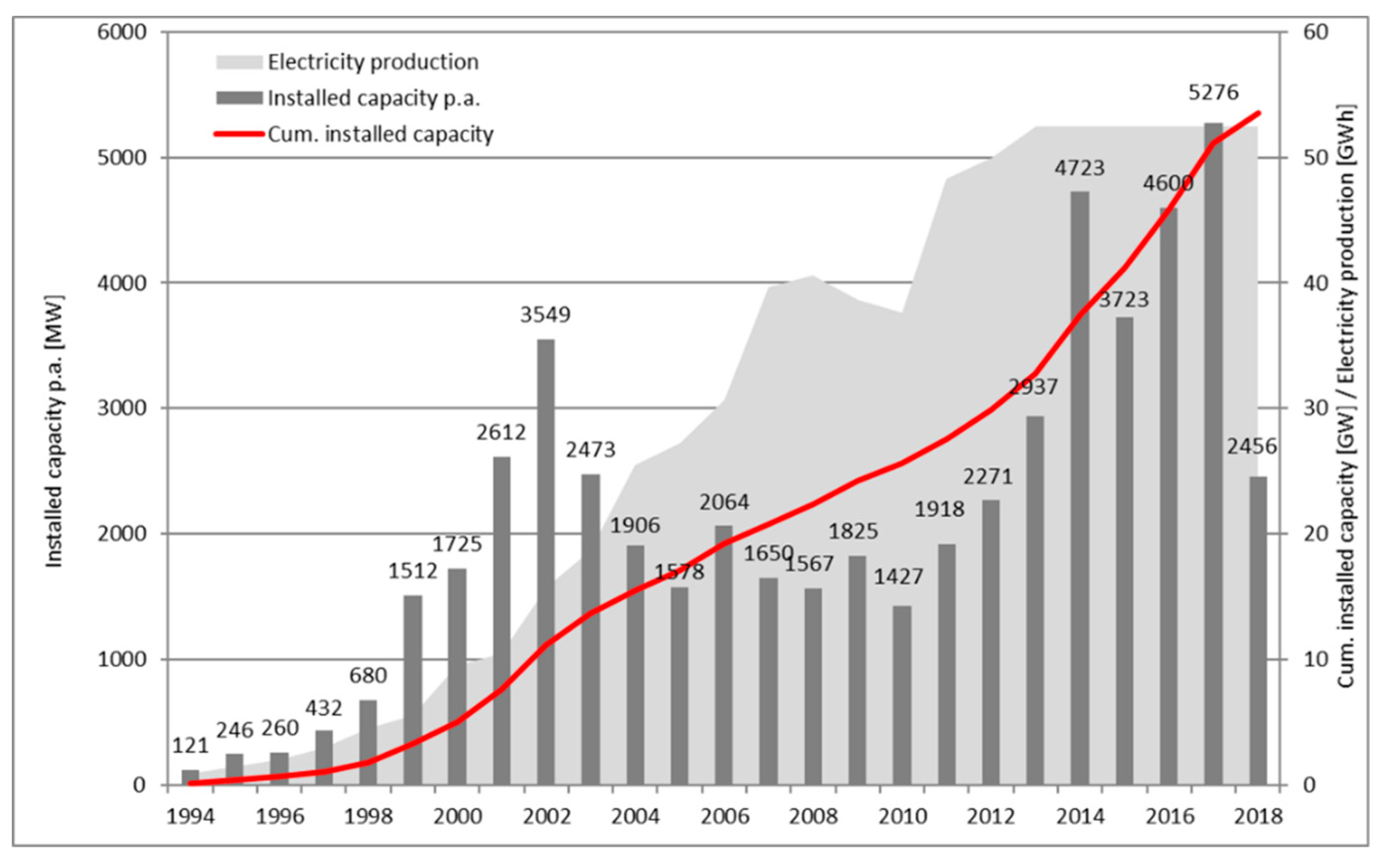
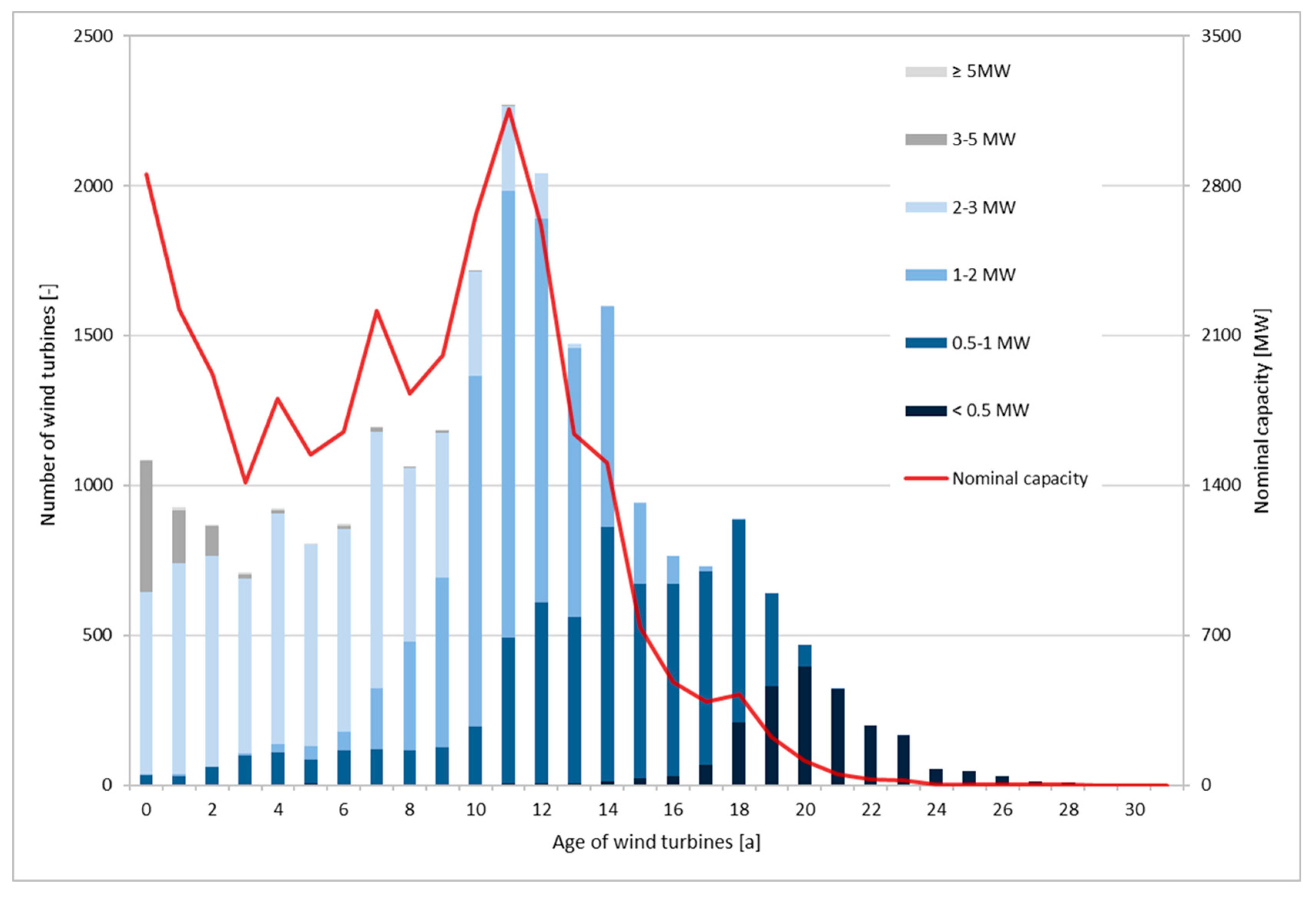
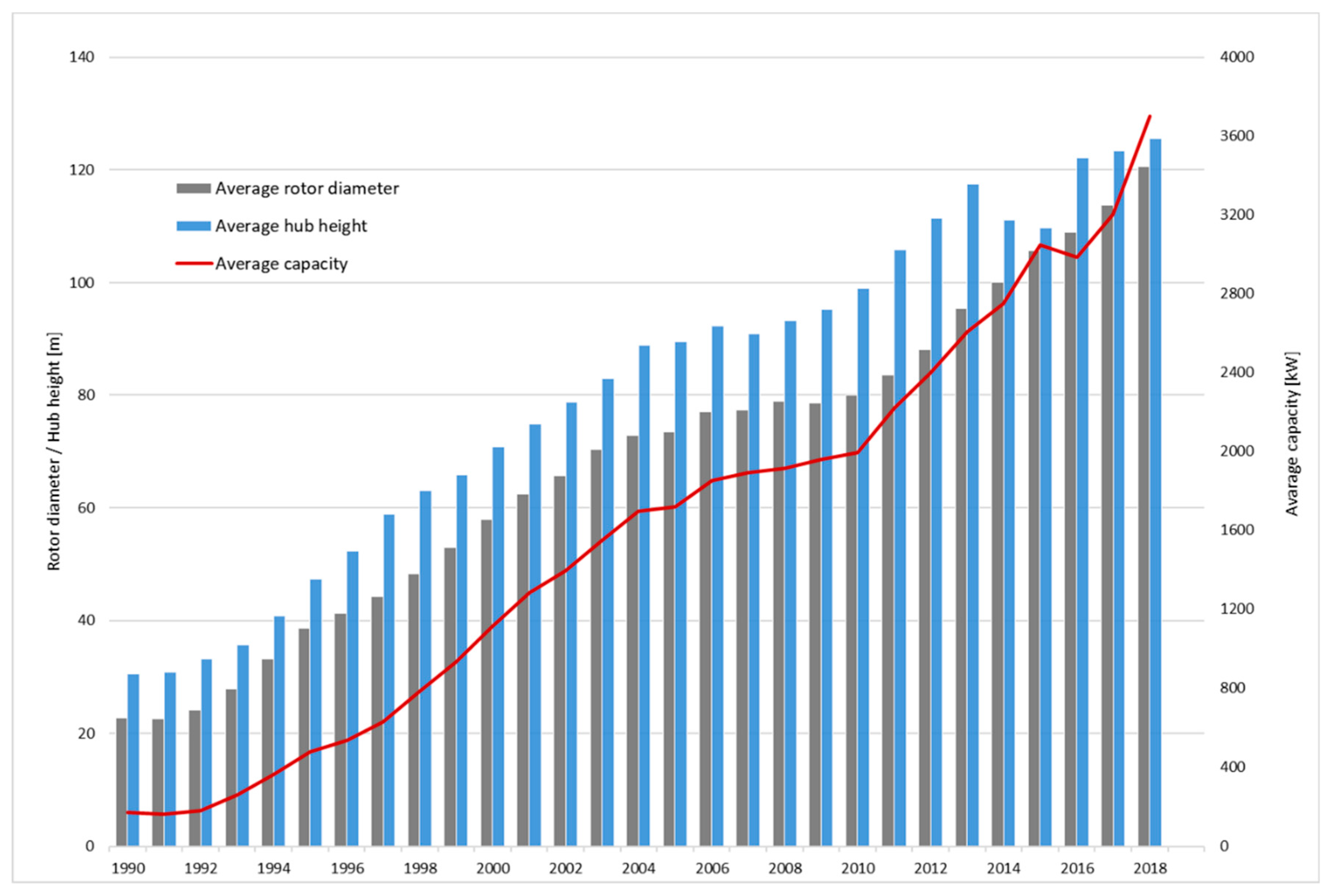
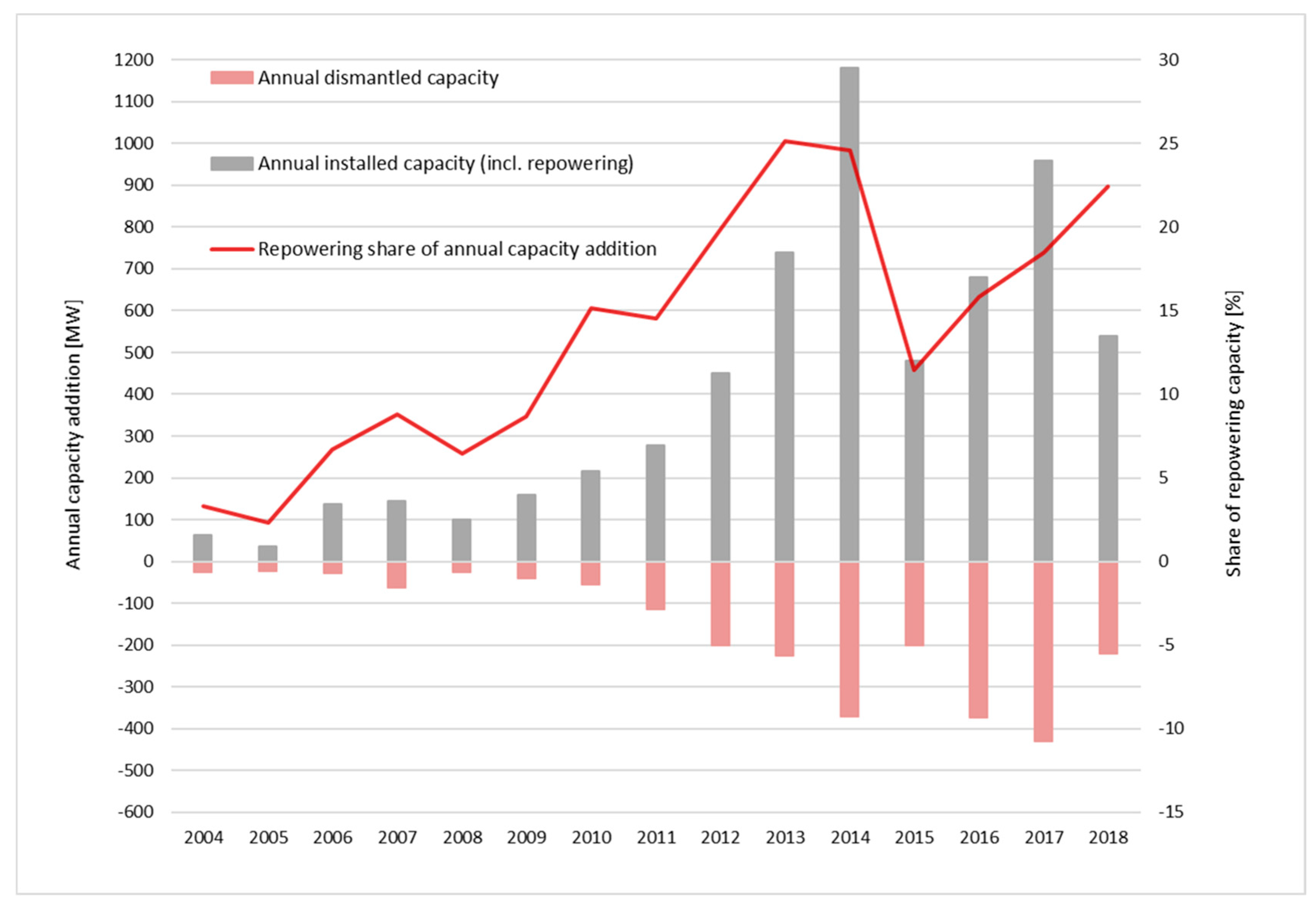
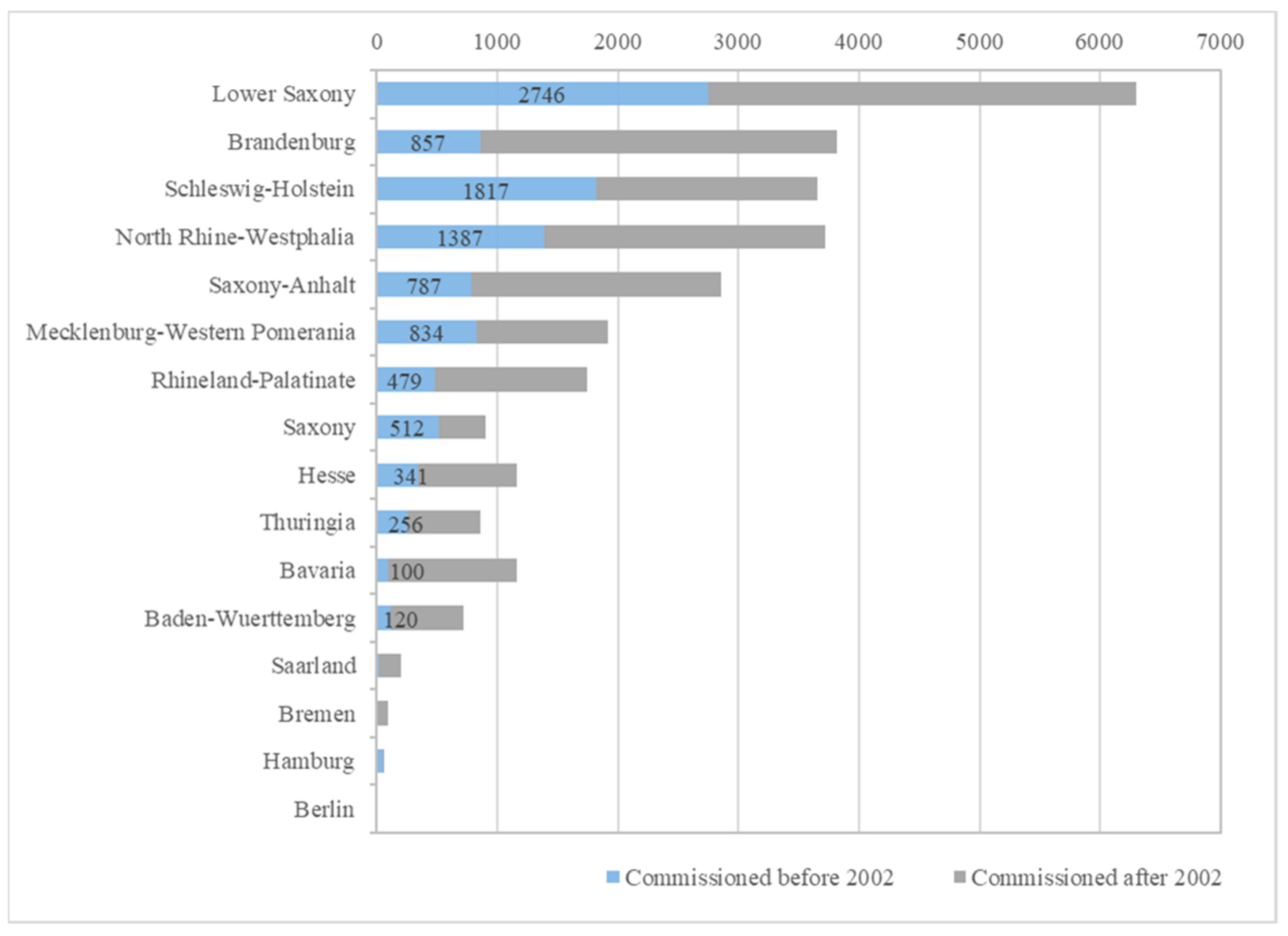
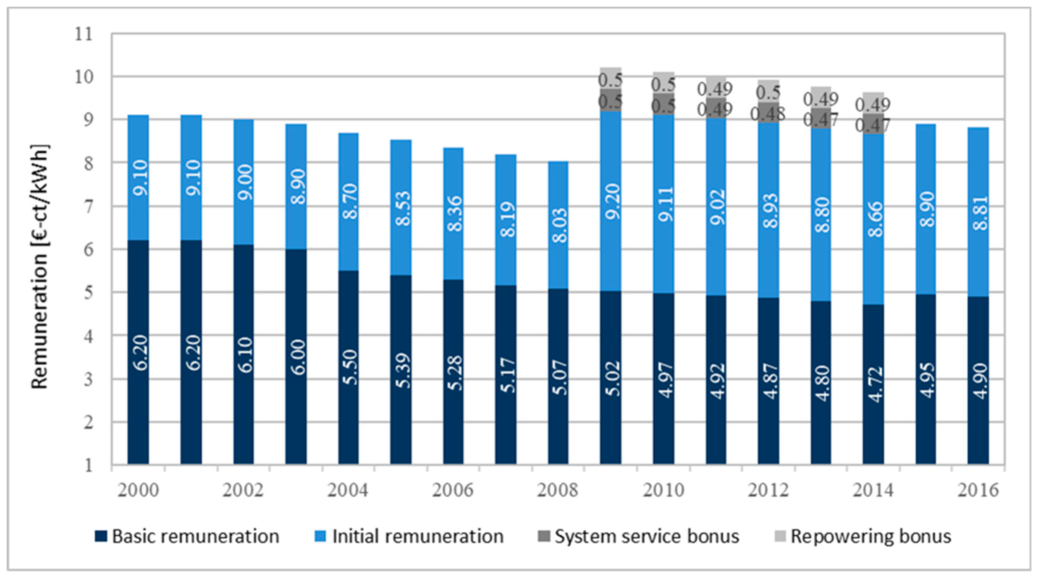
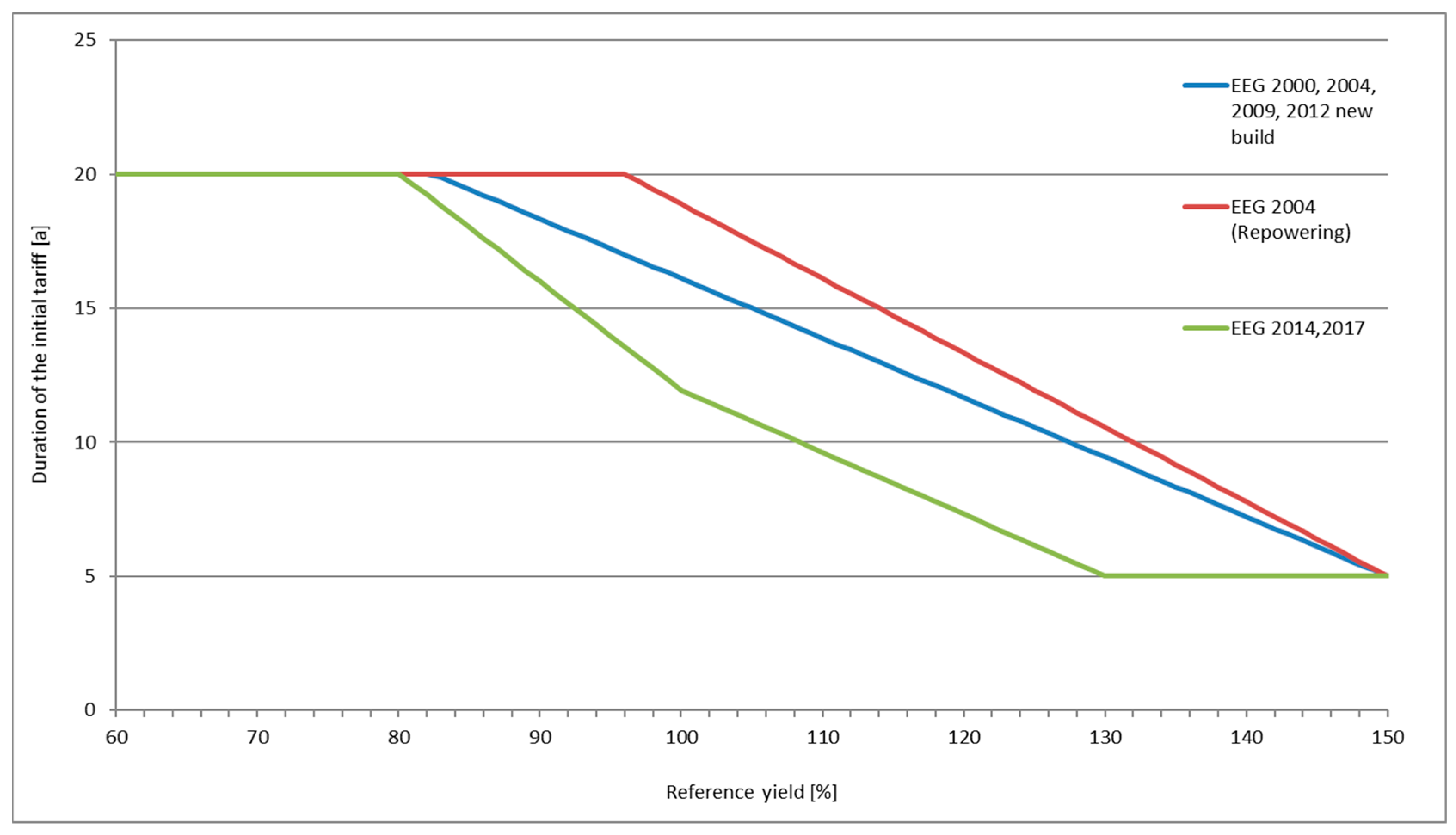
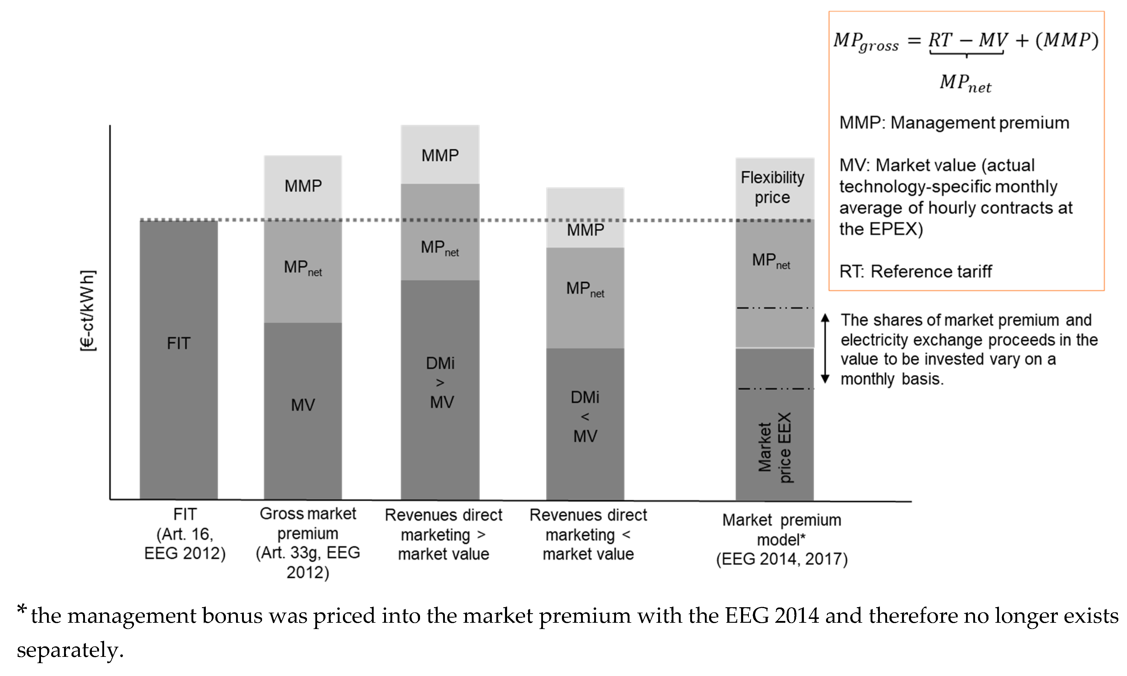
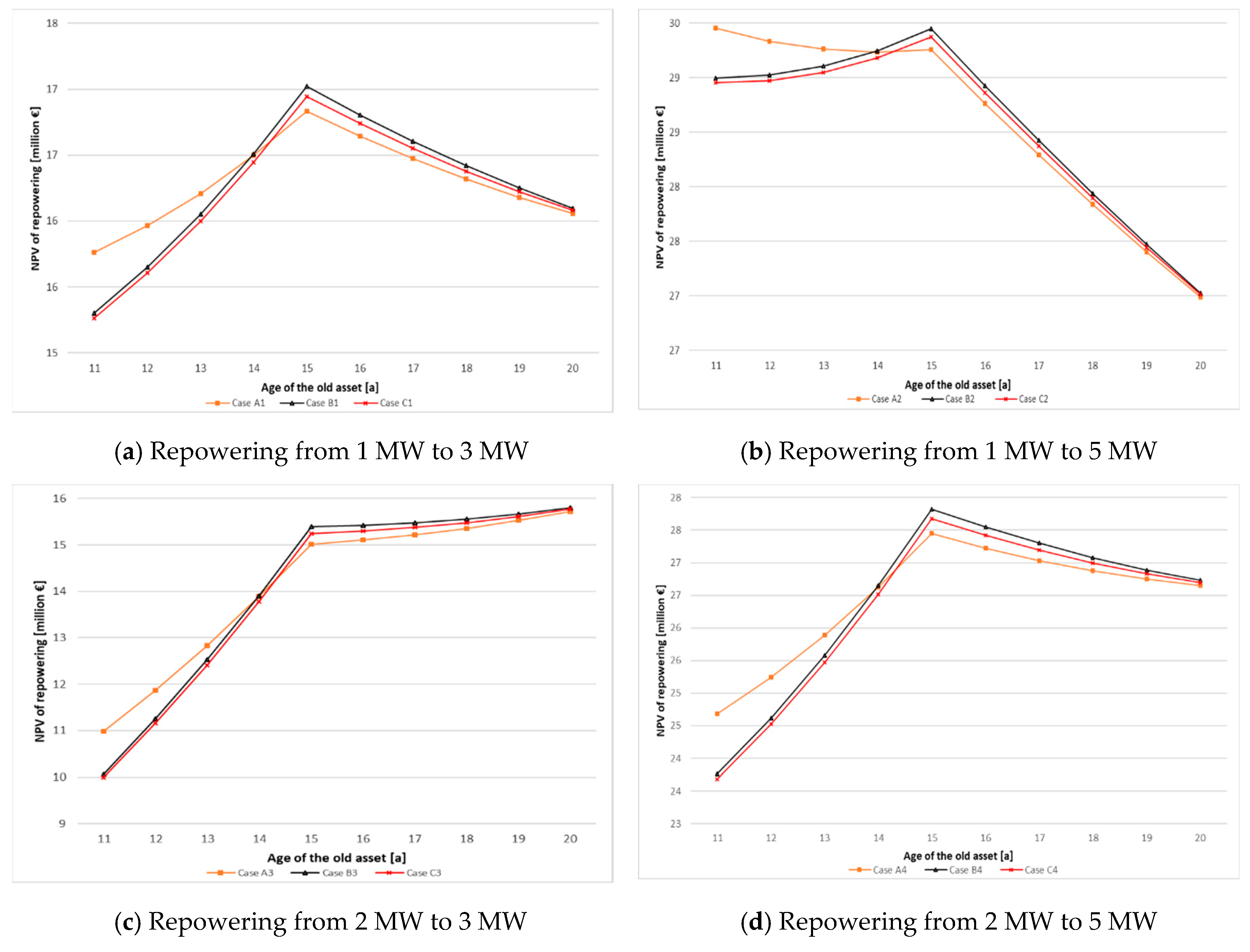
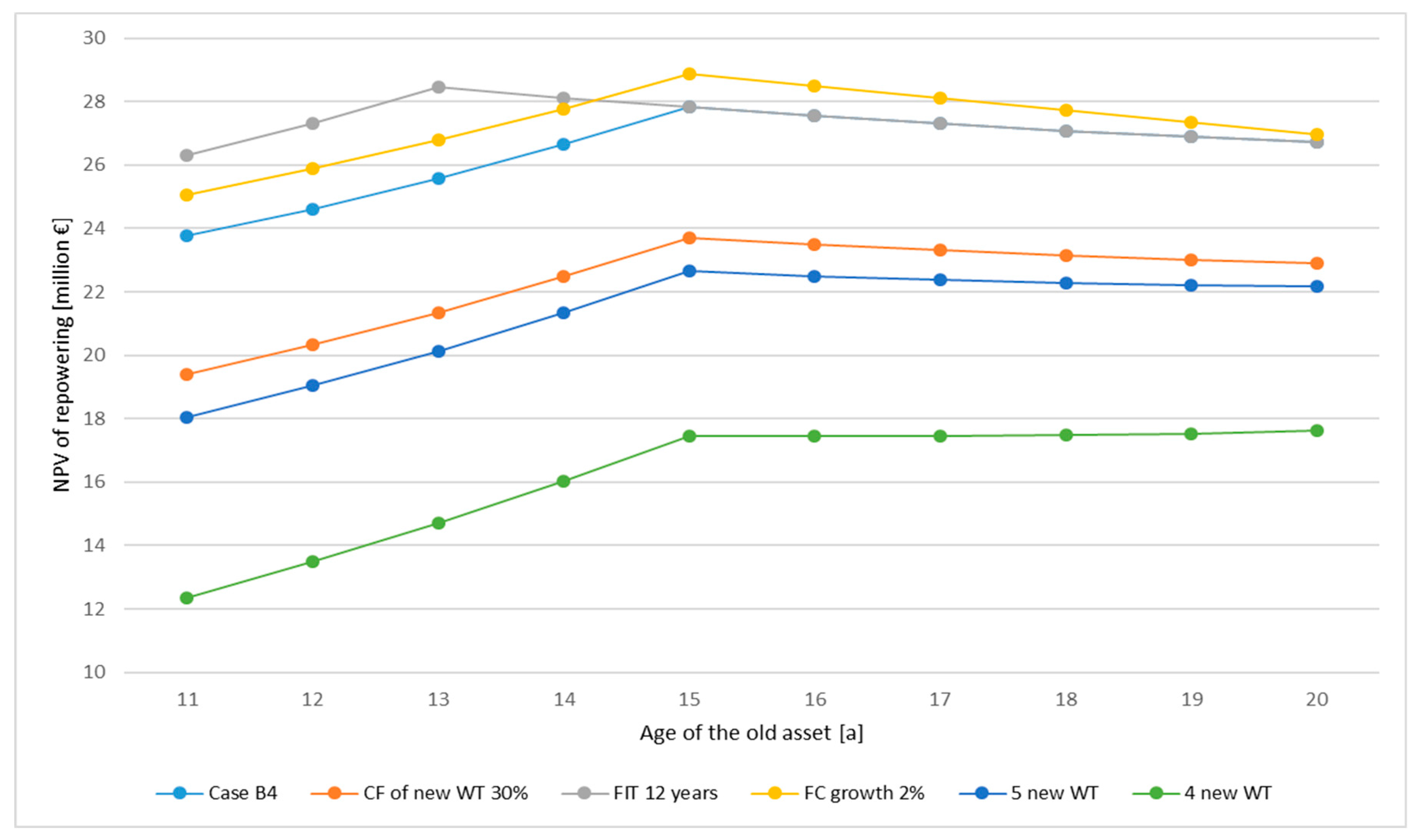
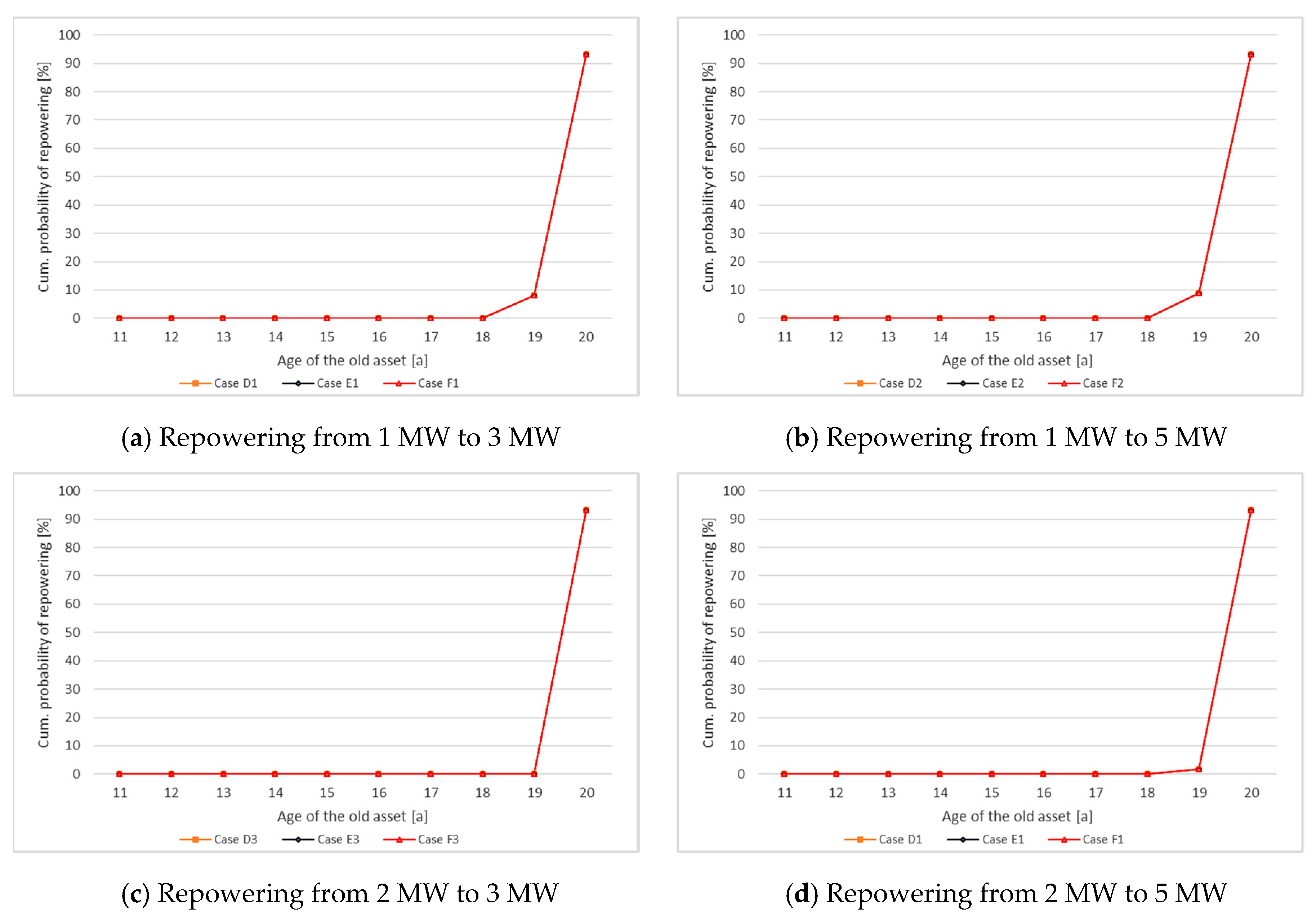
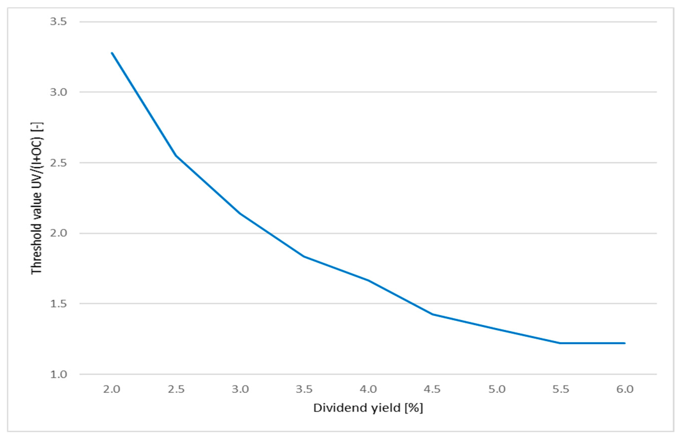
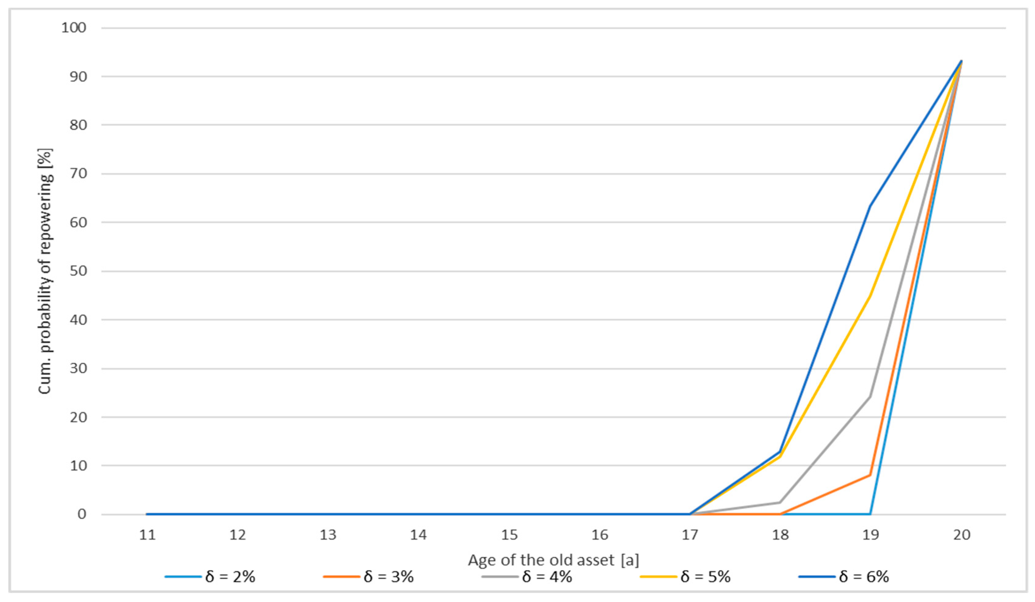
Figure 9.
Comparison of NPVs obtained from the repowering project for all A–C cases.

Figure 10.
NPV of the repowering project B4 case by age of the old WT asset and sensitivity analysis.
Figure 10.
NPV of the repowering project B4 case by age of the old WT asset and sensitivity analysis.

Figure 11.
Cumulative probability of repowering for all D–F case.

Figure 12.
Impact of the dividend yield on the threshold value for case D1.

Figure 13.
Cumulative probability of repowering at the end of a year depending on δ for case D1.

Table 1.
Repowering project Galmsbüll.
| Characteristics | Before Repowering | After Repowering |
|---|---|---|
| Number of wind turbines | 38 | 21 |
| Installed capacity | 12.4 MW | 60 MW |
| Electricity produced | 25,000 MWh/a | 155,000 MWh/a |
Source: Own illustration, based on [26].
Table 2.
Repowering cases regarding market premium model.
| Repowering from–to | Switch to Market Premium Model From | ||
|---|---|---|---|
| EEG 2008 | EEG 2012 | EEG 2014 | |
| 1 MW–3 MW | A1 | B1 | C1 |
| 2 MW–3 MW | A2 | B2 | C2 |
| 1 MW–5 MW | A3 | B3 | C3 |
| 2 MW–5 MW | A4 | B4 | C4 |
Table 3.
Repowering cases regarding free market regime.
| Repowering from–to | Switch to Free Market Regime From | ||
|---|---|---|---|
| EEG 2008 | EEG 2012 | EEG 2014 | |
| 1 MW–3 MW | D1 | E1 | F1 |
| 2 MW–3 MW | D2 | E2 | F2 |
| 1 MW–5 MW | D3 | E3 | F3 |
| 2 MW–5 MW | D4 | E4 | F4 |
Table 4.
Comparison of NPV of repowering (in million €) for different numbers of wind turbines (WT) after repowering across all defined cases.
Table 4.
Comparison of NPV of repowering (in million €) for different numbers of wind turbines (WT) after repowering across all defined cases.
| No. of WT After Repowering | Cases | |||
|---|---|---|---|---|
| A1–C1 | A2–C2 | A3–C3 | A4–C4 | |
| 6 | 15.3–17.0 | 27.0–29.5 | 10.0–15.8 | 23.7–27.8 |
| 5 | 11.8–13.9 | 22.4–24.3 | 6.6–13.1 | 18.0–22.7 |
| 4 | 8.4–10.6 | 17.6–18.0 | 3.1–10.3 | 12.3–17.6 |
Table 5.
Comparison of the cumulative probability of repowering for different numbers of wind turbines (WT) after repowering across all defined cases.
Table 5.
Comparison of the cumulative probability of repowering for different numbers of wind turbines (WT) after repowering across all defined cases.
| No. of WT After Repowering | Time of Repowering * | Cumulative Probability of Repowering [in %] For Cases: | |||
|---|---|---|---|---|---|
| D1–F1 | D2–F2 | D3–F3 | D4–F4 | ||
| 6 | 19 | 8.1 | 8.9 | - | 1.7 |
| 20 | 93.1 | 93.1 | 93.1 | 93.1 | |
| 5 | 19 | 1.7 | 8.1 | - | 1.5 (for D4 & F4)1.7 (for E4) |
| 20 | 93.1 | 93.1 | 93.1 | 93.1 | |
| 4 | 19 | 1.5 | 8.1 | - | 1.5 (for E4 & F4) |
| 20 | 93.1 | 93.1 | 93.1 | 93.1 | |
* equal age of the old asset [a].
© 2019 by the authors. Licensee MDPI, Basel, Switzerland. This article is an open access article distributed under the terms and conditions of the Creative Commons Attribution (CC BY) license (http://creativecommons.org/licenses/by/4.0/).
Share and Cite
MDPI and ACS Style
Madlener, R.; Glensk, B.; Gläsel, L. Optimal Timing of Onshore Wind Repowering in Germany under Policy Regime Changes: A Real Options Analysis. Energies 2019, 12, 4703. https://doi.org/10.3390/en12244703
AMA Style
Madlener R, Glensk B, Gläsel L. Optimal Timing of Onshore Wind Repowering in Germany under Policy Regime Changes: A Real Options Analysis. Energies. 2019; 12(24):4703. https://doi.org/10.3390/en12244703
Chicago/Turabian StyleMadlener, Reinhard, Barbara Glensk, and Lukas Gläsel. 2019. "Optimal Timing of Onshore Wind Repowering in Germany under Policy Regime Changes: A Real Options Analysis" Energies 12, no. 24: 4703. https://doi.org/10.3390/en12244703
Note that from the first issue of 2016, this journal uses article numbers instead of page numbers. See further details here.