Online Parametric Estimation of Grid Impedance Under Unbalanced Grid Conditions

Abstract

Whereas power-electronics-based power systems are expected to enable more integration of renewable energy sources, they could pose crucial challenges including stability issues due to the Thévenin impedance seen by inverters. Such problems could be mitigated by enabling the inverters to estimate the grid impedance by including a grid impedance estimation technique into their control loop. However, one aspect which has been overlooked thus far is that the accuracy of such grid impedance estimation techniques is significantly affected by various grid conditions. For instance, the unbalance in three-phase power systems causes unwanted oscillations at double the fundamental frequency in the inverters control loops. Therefore, this paper proposes a simple and reliable online estimation of the grid impedance under unbalanced conditions. The technique is based on wide-band impedance estimation incorporated into the control loop of the positive sequence of a three-phase grid-connected inverter equipped with a positive- and negative-sequence control (PNSC) strategy. Additionally, complex curve fitting is utilized to obtain parametric models of the grid impedance. To demonstrate the efficacy of the proposed grid impedance estimation technique, extensive case studies are performed. These include: (1) unbalanced operations of both resistive-inductive (RL) and resistive-inductive-capacitive (RLC) models of the grid, (2) background harmonics, and (3) asymmetrical impedances of the network.

1. Introduction

Potential stability issues [1,2] could be caused by a lack of grid impedance information in power-electronics-based power systems. Furthermore, there is a risk of negative impedance instability in converter-fed AC microgrids with high penetration of converter-interfaced loads because of strict power regulation [3]. The poor performance of the inverter-based distributed generation (DG) units due to variations of the grid impedance, especially the increase in the grid inductance, may also lead to unstable operation [4]. While the output impedance of inverters is determined by its design specifications [5], the major issue with the grid impedance is that it is a time-varying variable and it cannot be derived or measured directly at the the point of common coupling (PCC). Therefore, online estimation techniques should be adopted.

Recently, the online estimation of grid impedance by Photovoltaic (PV) inverters has become an appealing topic to many researchers for several reasons. Both active and passive grid impedance estimation techniques can be implemented into the control system of PV inverters [6]. This cost effective approach requires no extra hardware, such as a network impedance analyzer. The grid impedance information can be used to enhance the operation of grid-connected inverters, e.g., online stability analysis [7,8], voltage control [9], adaptive current controller [10], low voltage ride through [11], anti-islanding detection of grid-connected inverters [12,13,14,15], and analysis of multi-parallel inverters system [16,17,18].

A pseudo-random binary sequence (PRBS) has a spread-spectrum impedance estimation, and it has gained much interest as a nonparametric frequency response identification technique due to several advantages compared to other online wideband impedance estimation techniques implemented into the grid-connected inverters. It is a binary sequence with an optimal crest factor (equal to 1). It behaves as white noise, but it is generated easily using a deterministic algorithm. Moreover, it suits a practical implementation due to its small disturbance amplitude and immunity against background noise in the system [19,20]. Recently, the advantages of the PRBS have motivated researchers to adopt it for impedance estimation purpose while using power electronics converters [8,21,22,23,24,25].

The implementation of the PRBS identification technique into 3-phase grid-connected inverters controlled in the synchronous reference frames (dq-axis) for grid impedance estimation purpose has been reported in several studies [8,21,22,23]. The injection point of the PRBS in the control loop of the inverters differs between studies. For instance, it is injected into the carrier frequency of PWM [21], inner current controller references at dq-axis [22,23], and several locations (hybrid injection) simultaneously [8]. The second approach has the advantage of more control of the PRBS, and it provides more accurate results for a frequency range within the controller bandwidth. It is worth noting that all above studies on PRBS assumed balanced grid voltage conditions.

Several control techniques of grid-connected inverters have been realized in the dq-axis due to its simplicity and the direct relation between dq-axis currents and the injected active and reactive power to the grid. Therefore, most of the previous studies used the PRBS estimation technique to obtain the grid impedance in the dq-axis, where a single control loop was deployed to control the d- and q- components. However, the occurrence of an unbalanced grid voltage will produce an uncontrollable oscillation in the dq-axis at double the grid fundamental frequency [26]. In such a scenario, the grid impedance cannot be measured directly in the dq-axis unless indirect and more complicated techniques are utilized. Therefore, advanced control strategies should be adopted to ensure safe operation of the grid-connected inverters under unbalanced grid conditions [27]. Moreover, the implementation of the PRBS into the control loop of such advanced control strategies of grid-connected inverters for grid impedance estimation propose has not been reported in the literature.

Furthermore, background harmonics are usually presented in the grid voltage in the normal operation of low-voltage distribution network. The source of such harmonics are mainly nonlinear loads, power electronics converters, and variable-frequency drives [28]. Such harmonics may result in large estimation errors of the estimated grid impedance using grid-connected inverters. A common practice in overcoming this problem is to assume that the harmonic content in the grid voltage does not change in time. Therefore, pre-injection (unperturbed) measurements were subtracted from the captured (perturbed) measurements during signal injection (i.e., the PRBS) for the same window length [29,30]. However, if the background harmonics change during the estimation process (i.e., nonstationary harmonics and phase-shifted harmonics), the above procedure of subtraction of the unperturbed measurements from perturbed measurements will not be feasible. Hence, to consider more realistic scenarios for low-voltage distribution networks, more investigations are needed to explore the harmonics effects on the estimation accuracy based on the PRBS technique.

Although the grid impedance estimation based on the PRBS technique implemented in the dq-axis has been reported in the abovementioned works, all of them considered only inverters with single current loop. As a result, the overall estimation procedure of those approaches is either limited by the balanced operation of the network or need more complicated approaches to extract the impedance under unbalanced conditions, which tends to be impractical for online identification purposes. Therefore, it becomes necessary to explore online grid impedance estimation using grid-connected inverters in unbalanced low-voltage networks. Applications of the estimated impedance may include (1) online stability assessment based on generalised nyquist criteria to extend previous studies that considered the PRBS estimation technique only for balanced systems [7,21,22,23] and (2) the use of the fundamental grid impedance to improve, for example, low-voltage ride-through capability of grid-connected inverters. In recent studies [11,31], it was shown that the fundamental grid impedance components ($R_g$ and $L_g$) are required to obtain optimal or suboptimal dq-axis current references of both the positive- and negative sequences’ control loops. The work in the above studies assumed the information of the grid impedance is known and time-invariant, where this is not the case due to the dynamic properties of the power system, especially low-voltage distribution networks.

This paper proposes a robust and simple online wideband grid impedance estimation approach using the PRBS technique to include the operation of grid-connected inverters under unbalanced grid conditions. To do so, an advanced control strategy of grid-connected inverters called positive- and negative-sequence control (PNSC) strategy [32] is deployed. Further, its control loop is reconfigured to allow the PRBS injection on top of the d-axis current reference of the positive sequence. Finally, the impedance is estimated in the sequence domain based on the available voltage and current measurements at the PCC. Furthermore, complex curve fitting [33] is applied to obtain the parametric model of the grid impedance. The latter is important to overcome the challenge of frequency shift in the diagonal terms of the positive and negative sequences which are caused by the presence of the grid fundamental frequency [34]. This frequency shift causes substantial errors in the estimated fundamental grid impedance once it is performed in the sequence domain (or the natural reference frame (abc domain)). The proposed technique is summarized as follows:

• estimates the parametric model of the grid impedance under both balanced and unbalanced systems. The estimation algorithm is implemented into the control loop of grid-connected inverter equipped with PNSC strategy;
• takes into account both resistive-inductive (RL) and resistive-inductive-capacitive (RLC) models of the low-voltage distribution network;
• considers asymmetrical line impedances of the distribution network;
• assesses the estimation performance in the presence of background harmonics in the grid voltage;
• evaluates the effects of the initialization parameters of the curve-fitting algorithm on the accuracy of the obtained parametric model. These parameters are the PRBS frequency resolution ($f_{res}$), the number of selected data points (N), and the minimum frequency of selected data points to be fitted ($f_{min}$).

The paper is organized as follows: Section 2 describes the system under consideration including the control structure of the PNSC strategy of grid-connected inverters. Section 3 elaborates on the methodology of wideband and complex curve fitting of the grid impedance estimation based on the PRBS. Section 4 presents selected simulation results. Finally, Section 5 concludes the paper.

2. System Description

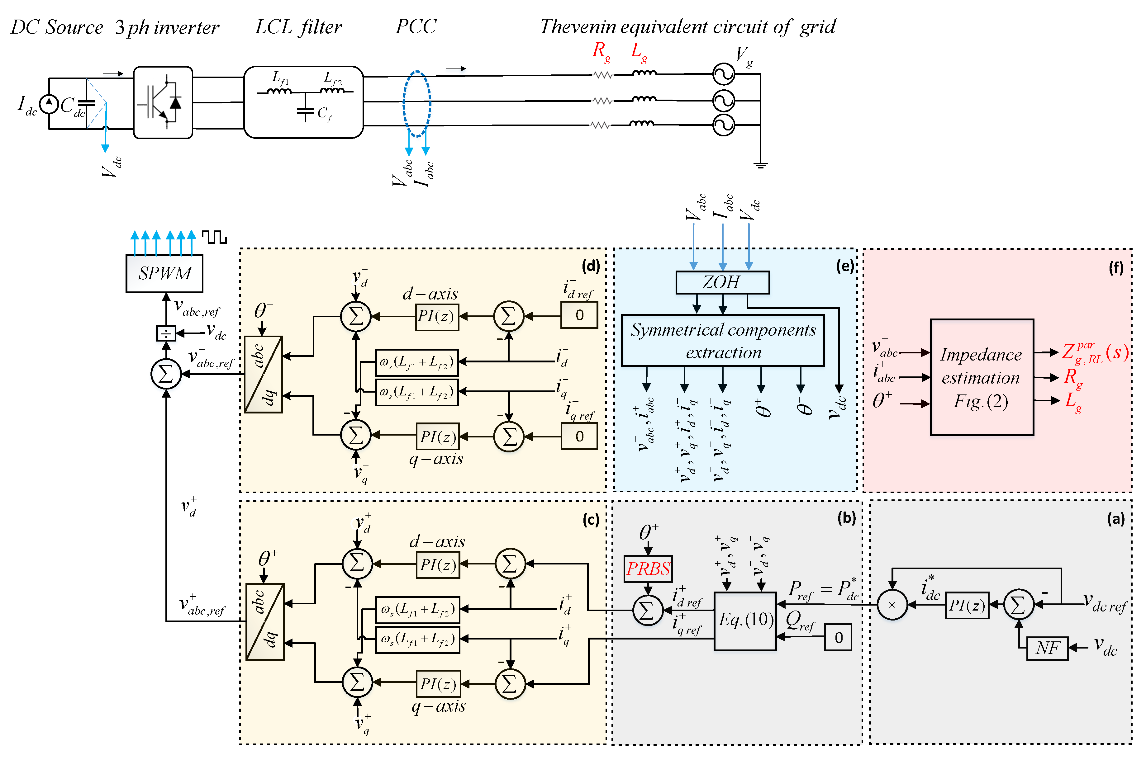
The 3-phase 3-wire inverter system under investigation is described in Figure 1, and the system parameters are listed in

Table 1. Simulation parameters of the system.

Description	Symbol	Values
Circuit parameters
Grid voltage (L-L, RMS)	$V_g$	400 V
Grid voltage frequency	$f_s$	50 Hz
Grid impedance (RL model)	$R_g,L_g$	0.5 $\Omega$, 0.5 mH
Grid impedance (RLC model)	$R_g,L_g,C_g$	2.5 $\Omega$, 1 mH, 3 $\mathsf{\mu }$F
DC current source	$I_{dc}$	7.3 A
DC bus reference voltage	$v_{dcref}$	700 V
Inverter rated active power	$P_{rated}$	5 kW
Inverter rated current (L-L, max)	$I_{max}$	10.2 A
Inverter-side filter inductance	$L_{f1}$	3 mH
Grid-side filter inductance	$L_{f2}$	0.6 mH
Filter capacitor	$C_f$	4 $\mathsf{\mu }$F
Damping resistance	$R_d$	3.7 $\Omega$
Control parameters
Switching frequency	$f_{sw}$	10 kHz
Sampling frequency	$f_s$	20 kHz
Notch filter frequency	$f_{NF}$	100 Hz
Inner current controller gains	$K_p,K_i$	30, 3000
Outer voltage controller gains	$K_p,K_i$	0.503, 30
SRF-PLL controller gains	$K_p,K_i$	1.74, 500

. The grid-connected inverter is equipped with a DC power supply to emulate a PV array. The inverter is interfaced into the utility grid through a passively damped LCL filter with wye connected filter capacitors. Discrete-time control based on proportional-integral (PI) controllers is deployed to regulate the DC link voltage and the positive and negative sequences. All measurements ($V_{abc}$, $I_{abc}$, and $V_{dc}$) are passed to the discrete-time control system through zero-order holders (ZOH) to highlight the possible limitations of discrete-time implementation of the PRBS technique. Furthermore, inverter switches are controlled using gate signals generated by the sinusoidal pulse width modulation (SPWM) technique.

The utility grid is represented by an equivalent Thévenin model, with a line-to-line root-mean-square (RMS) voltage of 400 V. This model includes the grid voltage source $V_g$ and the equivalent grid impedance $Z_g$. The work in this paper considers two different models of the $Z_g$. In the first model, the $Z_g$ is represented as series RL model. However, the second model of the $Z_g$ considers the RLC model. It is represented by a series resistance and inductance ($Z_1=R_g+s{L}_g$) in parallel with a capacitance ($Z_2=1/s{C}_g$) [8].

It is worth mentioning that only the RL model is shown in Figure 1. The equivalent transfer functions of the grid impedances for both the RL ($Z_{g,RL}\left(s\right)$) and RLC ($Z_{g,RLC}\left(s\right)$) models are given in Equations (1) and (2), respectively.

$$Z_{g,RL}\left(s\right)=R_g+s{L}_g$$

(1)

$$Z_{g,RLC}\left(s\right)=Z_1//Z_2=\frac{R_g+s{L}_g}{1+R_g{C}_{g}s+L_g{C}_g{s}^2}$$

(2)

The PNSC strategy ensures safe operation of the inverter by injecting only positively balanced current to the grid in both cases of balanced and unbalanced grid voltage conditions. In this paper, the control scheme of the inverter is modified to allow online wideband grid impedance estimation. The operation of grid-connected under unbalanced grid voltage, symmetrical components extraction, and the inner current control loops of the PNSC strategy are highlighted in the following subsections.

2.1. Operation of Grid-Connected Inverters under Unbalanced Grid Voltage Equipped with PNSC Strategy

During the normal operation of the grid-connected inverters, only the positive components of the grid voltage will be present in the system. However, the negative sequence component will appear once the unbalanced grid voltage occurs. In this case, the inverter output apparent power (S), function of active power (P), and reactive power (Q) are given by Equation (3) based the instantaneous PCC voltage ($v_{abc}$) and the instantaneous inverter output current ($i_{abc}$). By neglecting the zero sequence due to the adopted 3-phase 3-wire system as shown in Figure 1, the inverter output apparent power is given in Equation (4) as a function of the dq-components of the positive voltage ($v_{dq}^{+}$), the negative voltage ($v_{dq}^{-}$), the positive current ($i_{dq}^{+}$), and the negative current ($i_{dq}^{-}$).

$$S=P+jQ=v_{abc}\times i_{abc}^{*}$$

(3)

$$S=(v_{dq}^{+}{e}^{j\omega t}+v_{dq}^{-}{e}^{-j\omega t}){(i_{dq}^{+}{e}^{j\omega t}+i_{dq}^{-}{e}^{-j\omega t})}^{*}$$

(4)

The instantaneous apparent power is further separated into active power P(t) and reactive power Q(t) by

$$P\left(t\right)=P_0+P_{c2}cos\left(2\omega t\right)+P_{s2}sin\left(2\omega t\right)$$

(5)

$$Q\left(t\right)=Q_0+Q_{c2}cos\left(2\omega t\right)+Q_{s2}sin\left(2\omega t\right)$$

(6)

where $P_0$ and $Q_0$ are the average active and reactive injected by the inverter into the grid. It can be seen that the presence of the negative sequence caused by unbalanced occurrence resulted in oscillation at twice of the fundamental frequency $2\omega$ in both the active ($P_{s2}$, $P_{c2}$) and reactive power ($Q_{s2}$, $Q_{c2}$). The power is given as a function to dq currents as follows [27]:

$$\left[\begin{array}{c}P\\ Q\\ P_{c2}\\ P_{s2}\\ Q_{c2}\\ Q_{s2}\end{array}\right]=\frac{3}{2}\left[\begin{array}{ccccc}& v_d^{+}& v_q^{+}& v_d^{-}& v_q^{-}\\ & v_q^{+}& -v_d^{+}& v_q^{-}& -v_d^{-}\\ & v_d^{-}& v_q^{-}& v_d^{+}& v_q^{+}\\ & v_q^{-}& -v_d^{-}& -v_q^{+}& v_d^{+}\\ & v_q^{-}& -v_d^{-}& v_q^{+}& -v_d^{+}\\ & -v_d^{-}& -v_q^{-}& v_d^{+}& v_q^{+}\end{array}\right]\left[\begin{array}{c}{i}_d^{+}\\ i_q^{+}\\ i_d^{-}\\ i_q^{-}\end{array}\right]$$

(7)

For a grid-connected inverter equipped with the PNSC strategy implemented in the dq-axis, the current controller references can be obtained from Equation (8) based on the desired power (known values) to be injected to the grid by the inverter Equation (8) [35]:

$${\left[\begin{array}{c}{i}_d^{+}\\ i_q^{+}\\ i_d^{-}\\ i_q^{-}\end{array}\right]}_{ref}=\frac{2}{3}\left[\begin{array}{ccc}& v_d^{+}/E1& v_q^{+}/E2\\ & v_q^{+}/E1& -v_d^{+}/E2\\ & -K{v}_d^{-}/E1& +K{v}_q^{-}/E2\\ & -K{v}_q^{-}/E1& -K{v}_d^{-}/E2\end{array}\right]{\left[\begin{array}{c}P\\ Q\end{array}\right]}_{ref}$$

(8)

where,

$$\begin{array}{c}\hfill E1={\left(v_d^{+}\right)}^2+{\left(v_q^{+}\right)}^2-K({\left(v_d^{-}\right)}^2+{\left(v_q^{-}\right)}^2)\\ \hfill E2={\left(v_d^{+}\right)}^2+{\left(v_q^{+}\right)}^2+K({\left(v_d^{-}\right)}^2+{\left(v_q^{-}\right)}^2)\end{array}$$

(9)

and K is included in Equations (8) and (9), which have three possible real values, [0, 1, or −1]. It is used to determine the control objective as follows:

• K = 0: the inverter delivers a balanced current even under unbalanced voltage conditions. In this case, the negative current component references should be set to zero.
• K = 1: the inverter delivers active power free of oscillations.
• K = −1: the inverter delivers reactive power free of oscillations.

It can be seen that the first step to realize the PNSC strategy in the dq-axis is to extract the positive and negative sequences of the measured voltage and current at the PCC. In the literature, two different approaches are distinguished. In the first approach [26,32], the measurements are directly locked to the dq-axis with ${\omega }_{s}t$ and $-{\omega }_{s}t$. The second approach decomposes the measurements in the natural reference frame (abc domain) into their symmetrical sequences and then locks them to the dq-axis with ${\omega }_{s}t$ and $-{\omega }_{s}t$. This task is achieved by a symmetrical component extractor. The first approach is simple but introduces oscillations in the dq-axis at $2{\omega }_s$. Therefore, additional control approaches such as a notch filter and decoupling terms are reported to damp these oscillations. In contrast, the second approach will result in complete decoupling of the sequences in the dq-axis. However, the main drawback of the second approach is the introduced time delay that is required to decompose the sequences at the moment unbalance occurs. The authors of References [36,37] proposed fast techniques to extract the symmetrical components within one-fourth of the fundamental period, i.e., a 5-ms delay for a 50-Hz system. The second approach is used in our paper to extract the symmetrical components. Additionally, some modifications are applied, such as the implementation of a Synchronous Reference Frame Phase-locked loop (SRF-PLL).

2.2. Inner Current Control Loops of the PNSC Strategy

The PNSC is used to control the positive and negative sequences separately. Therefore, two control loops are used, namely a positive-sequence control loop and a negative-sequence control loop. Each control loop ensures that the inverter output current components follow their desired current references in the dq-axis. To enable the inverter to inject only balanced current, the dq-axis current references of the positive sequence ($i_{d_{ref}}^{+},i_{q_{ref}}^{+}$) are obtained from Equations (8) and (9) by considering K = 0 (similar analysis can be explored for the other two cases for K = 1 and K = −1) and by setting $Q_{ref}=0$. In this case, both the dq-axis current references of the negative sequence ($i_{d_{ref}}^{-},i_{q_{ref}}^{-}$) are set to zero. The dq-axis current references of the positive and negative control loops are given in Equations (10) and (11). Moreover, since there is no path for the zero sequence, it is not considered in the control loop.

$${\left[\begin{array}{c}{i}_d^{+}\\ i_q^{+}\end{array}\right]}_{ref}=\frac{2}{3}\left[\begin{array}{ccc}& \frac{v_d^{+}}{{\left(v_d^{+}\right)}^2+{\left(v_q^{+}\right)}^2}& \frac{v_q^{+}}{({v_d^{+})}^2+{\left(v_q^{+}\right)}^2}\\ & \frac{v_q^{+}}{{\left(v_d^{+}\right)}^2+{\left(v_q^{+}\right)}^2}& \frac{-v_d^{+}}{{\left(v_d^{+}\right)}^2+{\left(v_q^{+}\right)}^2}\end{array}\right]{\left[\begin{array}{c}P\\ Q\end{array}\right]}_{ref}$$

(10)

$$i_{d_{ref}}^{-}=i_{q_{ref}}^{-}=0$$

(11)

3. Wideband Grid Impedance Estimation Under Unbalanced Grid Voltage

The methodology followed in this paper for the wideband estimation and parametric identification of grid impedance using a grid-connected inverter equipped with the PNSC strategy is presented as follows:

3.1. PRBS Disturbance Injection by the PNSC Strategy

The PRBS is a periodic wideband identification technique. Among PRBS signals, a maximum length binary sequence (MLBS) is the most commonly used due to the simple implementation using feedback shift registers [19]. The MLBS is used in our paper and it is implemented in MATLAB/Simulink based on a 10-bit generator using a unit delay. It has a frequency resolution $F_{res}$ = 1 Hz. Therefore, 1 s is the required time to inject one period of the PRBS to estimate the grid impedance. The PRBS parameters used are summarized in

Table 2. PRBS parameters.

Description	Symbol	Value
Bit-length of the PRBS generator	-	10-bit
Maximum length binary sequence	$MLBS$	1023 bits
Frequency resolution	$F_{res}$	1 Hz
Generator’s clock frequency	$F_{gen}$	1023 Hz
Injected disturbance amplitude	$I_{inj}$	6% $I_{max}$

.

To enable the inverter to estimate the grid impedance with an unbalanced grid voltage, the PNSC strategy is configured to allow the PRBS injection, as illustrated in Figure 1. The PRBS is added on top of the d-axis current reference of the positive sequence, calculated from Equation (10) based on the power reference generated by the outer voltage controller of the DC bus. To minimize its distortion effects on the inverter output waveforms and to obtain almost zero mean, the generated PRBS is scaled before it is added on top of the current reference [23].

3.2. Grid Impedance Estimation Based on PRBS Injection

Generally, the grid impedance estimation could be performed in different reference frames, namely dq domain, sequence domain, and/or abc domain. The first approach is preferred for balanced systems. For passive circuits, the d and q grid impedances are equal to each other. Therefore, it is sufficient for grid impedance estimation to measure d-impedance. However, the grid impedance estimation is no longer straightforward and it cannot be accurately identified due to the unbalanced conditions which, eventually, produces oscillations in the dq-axis signals at double the fundamental frequency. Hence, indirect and more complicated techniques could be used, such as the harmonic-transfer-function approach [38]. On the other hand, identifying the impedance in the sequence domain is simple and gives more reliable results under the unbalanced operation. The identification process is based on the analysis of the symmetrical components. Therefore, the second approach is implemented in this paper, where the online grid impedance estimation is performed in the sequence domain based on the voltage $(v_{abc}^{+}$) and current ($i_{abc}^{+}$) measurements of the positive sequence. The grid impedance in the sequence domain ($Z_g^{\pm }$) is given based on Equation (12) [39].

$$Z_g^{\pm }=\left[\begin{array}{cc}{Z}_g^{+}& 0\\ 0& Z_g^{-}\end{array}\right]$$

(12)

where $Z_g^{+}$ and $Z_g^{-}$ are the positive and negative impedances. The equivalent grid impedance at the sequence domain is related to the adopted model of the grid impedance whether RL or RLC models are used, as shown below.

The RL model of the grid impedance is a common practice where the low-voltage distribution network is represented by an equivalent impedance consisting of $R_g$ and $L_g$ to simplify the study of the system. The equivalent grid impedance in the sequence domain ($Z_{g,RL}^{\pm }$) is expressed as follows:

$$Z_{g,RL}^{\pm }=\left[\begin{array}{cc}{R}_g+(s+{\omega }_s)L_g& 0\\ 0& R_g+(s-{\omega }_s)L_g\end{array}\right]$$

(13)

where ${\omega }_s$ is the grid voltage angular frequency.

For the RLC model presented in Equation (2), the equivalent grid impedance is expressed in sequence domain ($Z_{g,RLC}^{\pm }$) by

$$Z_{g,RLC}^{\pm }=Z_1^{\pm }//Z_2^{\pm }=\left[\begin{array}{cc}\frac{R_g+(s+{\omega }_s)L_g}{D_1}& 0\\ 0& \frac{R_g+(s-{\omega }_s)L_g}{D_2}\end{array}\right]$$

(14)

where

$$\begin{array}{c}\hfill D_1=L_g{C}_g{(s+{\omega }_s)}^2+R_g{C}_g(s+{\omega }_s)+1\\ \hfill D_2=L_g{C}_g{(s-{\omega }_s)}^2+R_g{C}_g(s-{\omega }_s)+1\end{array}$$

(15)

From Equations (13) and (14), it can be seen that the cross-coupling terms are always zero while the diagonal terms are equal to the grid impedance but with a frequency shift. Therefore, when estimating the grid impedance in the sequence domain, we expect to see a resonance peak at 50 Hz corresponding to the presence of ${\omega }_s$ in the network. It is worth mentioning that the positive and negative impedances of the grid are identical ($Z_g^{+}=Z_g^{-}$) for passive electrical components such as cables/lines, which are considered in this paper. Therefore, a straightforward approach to characterize the grid impedance is to apply what is called harmonic linearization [1] at every desired frequency $\left(\omega \right)$. Here, the impedance identification is performed based on the positive-sequence measurements ($v^{+}\left(\omega \right)$, $i^{+}\left(\omega \right)$), as expressed in Equation (16).

$$Z{g}^{+}\left(\omega \right)=v^{+}\left(\omega \right)/i^{+}\left(\omega \right)$$

(16)

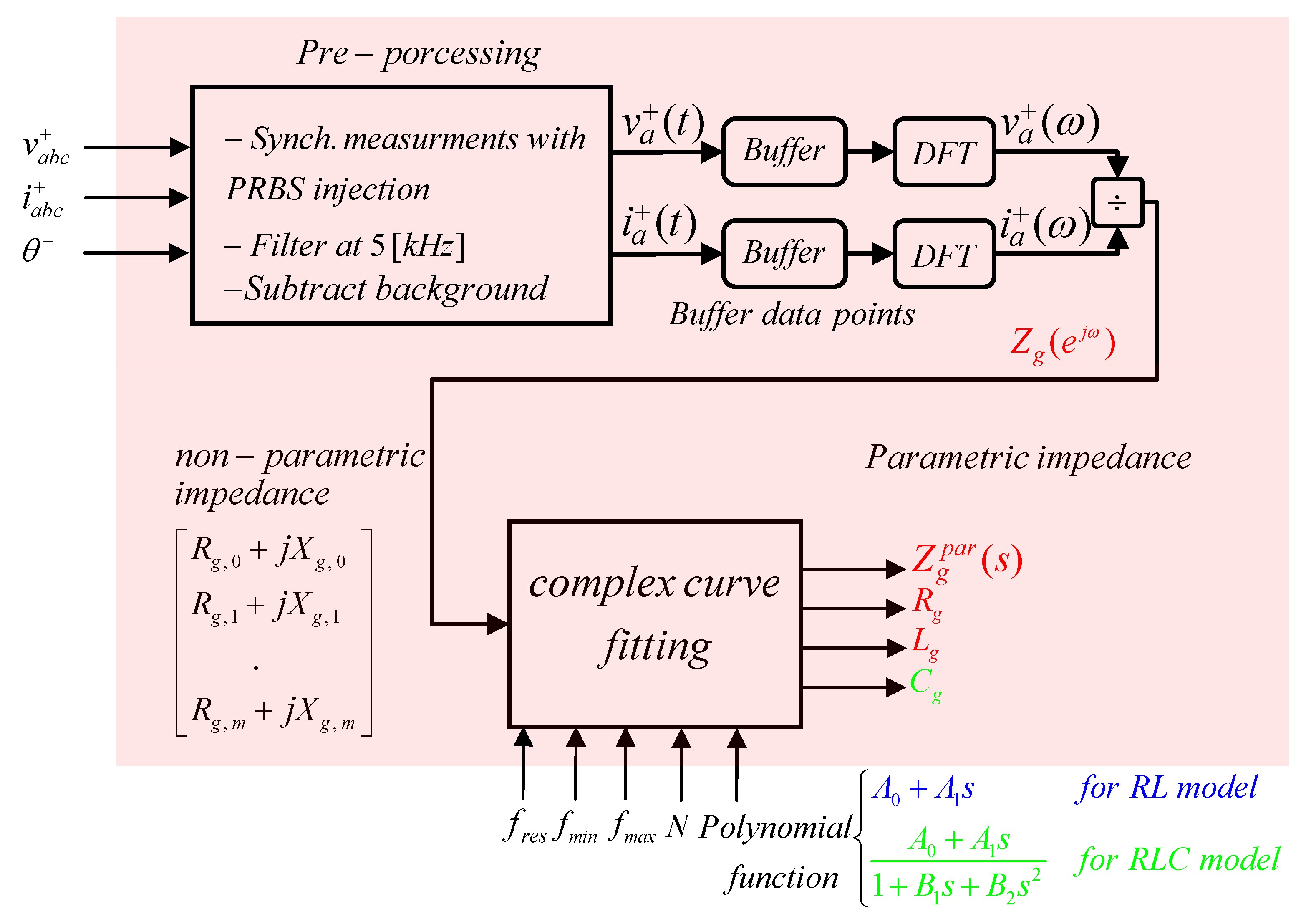
In this paper, the main steps to estimate the grid impedance followed by grid parametric identification are illustrated in Figure 2. The extracted symmetrical components of the inverter output current and the PCC voltage measurements are synchronized with the injected PRBS on top of $i_{dref}^{+}$. The synchronization is done based on the phase angle of the positive sequence. Then, these measurements are filtered using a low-pass filter with a cut-off frequency of 5 kHz, half of the inverter switching frequency. Furthermore, the subtraction of fundamental frequency and other background harmonics in the system were applied to enhance the estimation accuracy. This was accomplished by subtracting the recorded voltage and current measurements before applying PRBS from the perturbed measurements with the PRBS for the same window [40]. Next, Discrete Fourier transform (DFT) is applied to both buffered current and voltage vectors measurements of any phase, here, phase A, independently. Finally, Equation (16) is applied to obtain the impedance frequency response of the Thévenin model of utility grid $Z_g$ over the desired frequency range.

3.3. Parametric Impedance Based on Complex Curve Fitting

It was shown in Equations (13) and (14) that it is not applicable to find accurate values of the grid impedance in the sequence domain at the fundamental frequency. Even though the approach of subtracting fundamental and its background harmonics in the pre-processing stage was followed, it was proved in References [29,30] that this procedure will not completely remove their effects on the impedance estimation results. Therefore, the curve-fitting approach is a useful solution that could be followed to construct the mathematical transfer function of the grid impedance from a chosen series of data points at different frequencies.

The curve fitting for parametric grid impedance purpose was also adopted in References [8,39]. However, both studies have not considered the unbalanced operation of the power system. Besides, the implementation of the PNSC strategy for grid-connected inverters was not considered. Moreover, the authors of Reference [8] only deal with the RLC model of the grid impedance, where the complex curve-fitting technique was applied to dq impedances. Furthermore, it is not clear how the grid impedance components (R, L, and C) can be obtained from the fitted polynomial function. This paper utilizes the complex curve fitting in the sequence domain and abc domain. This enables a reliable, simple, and detailed parametric estimation of both RL and RLC models under both balanced and unbalanced grid conditions. The fitting technique relies on “the minimization of the weighted sum of the squares of the errors between the absolute magnitudes of the actual function and the polynomial ratio, taken at various values of frequency” according to Reference [33].

As shown in Figure 2, some initializations are required to use the complex curve-fitting algorithm. First is to define the used PRBS frequency resolution ($F_{res}$) and the frequency range of the data points to be fitted. The defined frequency range is between a minimum frequency ($f_{min}$) and a maximum frequency ($f_{max}$). The $f_{max}$ value should not exceed half of the inverter’s switching frequency. Second is to select the number of the data points (N) to be processed for the curve fitting, where a small number could affect the accuracy of the estimated coefficients and a large number increases the computational burden.

Table 3. Idealization values for the parametric impedance estimation algorithm.

Parameter	Symbol	Value
PRBS frequency resolution	$F_{res}$	1 Hz
Minimum frequency	$f_{min}$	10 Hz
Maximum frequency	$f_{max}$	5 kHz
No. of the data points for curve fitting	N	500

shows the default setting values of $F_{res}$, $f_{min}$, and N that are being used for the Results section. It is worth mentioning that the setting value of $F_{res}$ should be the same as the injected PRBS. Moreover, detailed case studies of the trade-off between the abovementioned parameters and the accuracy of the obtained parametric impedance will be explored in the results; see Section 4.1.3.

The third parameter required for the complex curve fitting is to define the chosen polynomial function for the curve fitting with respect to the equivalent grid impedance transfer functions in Equation (1) or Equation (2). For the RL model, the best candidate polynomial function for curve fitting ($Z_{g,RL}^{par}\left(s\right)$) is given in Equation (17).

$$Z_{g,RL}^{par}\left(s\right)=A_0+A_{1}s$$

(17)

where $A_0$ and $A_1$ are the transfer function coefficients that need to be identified. Then, the grid impedance components are obtained by comparing Equation (1) with Equation (17) as shown below.

$$\left\{\begin{array}{c}{R}_g=A_0\hfill \\ L_g=A_1\hfill \end{array}\right.$$

(18)

Similarly, the parametric grid impedance of the RLC model ($Z_{g,RLC}^{par}\left(s\right)$) is obtained after curve fitting is applied. Unlike RL model, a second-order polynomial function is chosen here with respect to Equation (2) as shown in Equation (19)

$$Z_{g,RLC}^{par}\left(s\right)=\frac{A_0+A_{1}s}{1+B_{1}s+B_2{s}^2}$$

(19)

where $A_0,A_1,B_1$, and $B_2$ are the transfer function coefficients that need to be estimated. Finally, the grid impedance components are obtained by comparing Equation (2) with Equation (19) as shown in Equation (20).

$$\left\{\begin{array}{c}{R}_g=A_0\hfill \\ L_g=A_1\hfill \\ C_g=B_1/A_0;\mathrm{or}{C}_g=B_2/A_1\hfill \end{array}\right.$$

(20)

4. Results and Discussion

To verify the proposed grid impedance estimation technique for an unbalanced grid, extensive simulation case studies are carried out. Figure 1 shows the simulated 3-phase 3-wire inverter system. The simulation parameters of the system, the PRBS parameters, and the idealization values of the parametric impedance estimation algorithm are given in Table 1, Table 2 and Table 3, respectively. The simulation has been implemented in MATLAB/Simulink environment, where piecewise linear electrical circuit simulation (PLECS) toolbox components are used for accurate modeling of power electronics components. Furthermore, a discrete-time control and estimation model is used for the estimation results in order to consider real sample measurements and to highlight the limitations of implementing a grid impedance estimation technique using PRBS.

The presented results considering both the RL and RLC models of the equivalent grid impedance of the low-voltage distribution network seen at the PCC of the grid-connected inverter are presented as follows. Section 4.1 provides insight to the estimation performance of the RL model for several cases, namely (1) for balanced network, (2) for unbalanced grid voltage with/without background harmonics, (3) for effects of the initialization parameters of the parametric algorithm ($F_{res}$, $f_{min}$, and N) on the accuracy of parametric grid impedance estimation, and (4) for asymmetrical line impedances of the distribution network. Additionally, Section 4.2 explores the RLC model, where the system under unbalanced grid voltage and asymmetrical line impedances is considered.

4.1. RL Model of the Equivalent Impedance of Low-Voltage Distribution Network

The simulation are carried out for both balanced and unbalanced grid voltage conditions for a simulation time of 3 s (with an exception when the PRBS frequency resolution is studied). To estimate the grid impedance, an injection of two PRBS periods to the system is applied from the simulation time equal to 1 s, where each period has a duration of 1 s. Next, the grid impedance is estimated from the synchronous voltage and current measurements of the positive sequence during the injection of the second PRBS period, and measurements of the first period are neglected for better estimation results (to remove the PRBS transient). Moreover, to improve the estimation accuracy, the unperturbed measurements with the PRBS are subtracted from perpetrated measurements for the same window length of the PRBS period; here, it is equal to 1 s. Finally, curve fitting is applied to find the parametric model of the grid impedance.

4.1.1. Balanced Distribution Network

For the balanced grid voltage scenario, Figure 3a shows the nonparametric estimation results of the grid impedance up to half of the switching frequency, $f_{sw}$ = 10 kHz. It can be noticed that there is a peak at around 50 Hz as it is expected in Equation (12). Moreover, the estimation accuracy deteriorates beyond the PRBS generator’s clock frequency, $F_{gen}$= 1023 Hz, since PRBS signals provide very accurate identification results up to one-third of its $F_{gen}$. Another constraint is $f_{sw}$, where the estimation results is limited to half of $f_{sw}$.

Therefore, to obtain a continuous model of the grid impedance, complex curve fitting is applied based on the desired polynomial function to be fitted; see Equation (17). The estimated nonparametric impedance data points from DFT is forwarded as an input for the curve-fitting algorithm. The algorithm is provided with the initialization values presented in Table 3. The selection of certain data points (N = 500 samples) out of 20,000 samples is achieved within the defined frequency range. The selected data points for curve fitting are shown in Figure 3a. Finally, the obtained parametric impedance from curve fitting is given in Equation (21). Therefore, the grid resistance and inductance values can be obtained easily with the aid of Equation (18). To verify the accuracy of the results, the parametric estimation results are compared with the analytical (reference) impedance, $Z_{gRL}\left(s\right)=0.5+0.5\times {10}^{-3}s$, as shown in Figure 3b. The estimation errors in the grid impedance components are $\Delta R=-6.4\%,\Delta L=-1.67\%$.

$$Z_{g,RL}^{par}\left(s\right)=0.468+0.491\times {10}^{-3}s$$

(21)

4.1.2. Unbalanced Grid Voltage

The operation under unbalanced grid voltage conditions is investigated for two scenarios, without and with background harmonics in the grid voltage. Figure 4 shows the first scenario representing the unbalanced condition without background harmonics for a voltage sag with an amplitude of 50% $V_g$ in phase B. Figure 4b shows the inverter with the PNSC strategy injecting only a balanced current. It is found that the occurrence of an unbalance of 50% $V_g$ voltage sag in phase B increases the inverter output current from 7.3 A to around 8.83 A in order to maintain the output power equal to its reference of 5 kW. Limiting strategies of the inverter output current should be adopted to consider fault conditions. However, this is limited to $1.5\times I_{max}$ since it is beyond the scope of this paper. Figure 4 also shows the PRBS injection effects on the PCC voltage, the inverter output current, the DC bus voltage, and the detected phase angle of the positive sequence. It is found that the PRBS injection causes an increase in the total harmonic distortion (THD%) of the inverter output current at the PCC by 3%. The THD is measured up to the 50th harmonics. Furthermore, the PRBS injection causes a slight ripple in the DC bus voltage, less than 1 V .

Unlike the first scenario, the second scenario examined the estimation accuracy of the grid impedance for unbalanced and polluted grid voltage source with harmonics. In this case, the processed voltage and current measurements for impedance identification contained the background harmonics. Figure 5a shows the simulated nonideal grid voltage source with unbalanced 50% $V_g$ voltage sag in phase B. It contains five different harmonics present with their maximum allowable amplitude according to the Australian harmonics standards [41]. The considered harmonics amplitudes are 5% for 3rd, 5th, and 7th; 1.5% for 9th; and 3.5% for 11th. The frequency harmonic spectrum of the equivalent Thévenin grid voltage at the PCC is shown in Figure 5b.

Figure 6a,b presents the estimated grid impedance for the unbalanced case study (50% voltage sag in phase B) without background harmonics. Overall, the performance of the proposed technique successfully estimates the grid impedance. Also, Figure 6b compares the analytical solution with the fitted curve. It can be seen that the utilization of curve fitting for impedance estimation provides accurate results, as shown in Equation (22). The estimation errors in the grid impedance components are $\Delta R=3.1\%,\Delta L=5.5\%$.

$$Z_{g,RL}^{par}\left(s\right)=0.515+0.527\times {10}^{-3}s$$

(22)

The above case studies of the obtained results of parametric grid impedance as a function of grid voltage conditions are summarized in

Table 4. A summary of the parametric grid impedance estimation as a function to the grid voltage conditions.

Case Study No.	Operation Scenario	Parametric Impedance	$\mathbf{\Delta }\mathit{R}\%$	$\mathbf{\Delta }\mathit{L}\%$
Case 1	Balanced	0.468 + 0.491$\times {10}^{-3}$ s	−6.4	−1.7
Case 2	Unbalanced	0.515 + 0.527$\times {10}^{-3}$ s	3.1	5.5
Case 3	Unbalanced	0.422 + 0.454$\times {10}^{-3}$ s	−15.6	−9.0

. The first case represents the balanced grid voltage while the second and third cases represent unbalanced operation without background harmonics. In the second case, the applied voltage sag to phase B is 50%. Furthermore, an additional case study is considered, case 3. It represents a severe operation when a voltage sag of 50% was applied to both phase B and phase C. The severe estimation errors are larger for the third case, especially for the real part.

On the other hand, Figure 6c,d show the estimated grid impedance case for a polluted grid voltage with background harmonics. Figure 6c shows the nonparametric impedance and the background harmonics which appear in the impedance spectrum at their corresponding frequencies. The parametric impedance shown in Figure 6d, is also given in Equation (23), where the estimation errors in the grid impedance components are $\Delta R=-0.8\%,\Delta L=1.8\%$.

$$Z_{g,RL}^{par}\left(s\right)=0.496+0.509\times {10}^{-3}s$$

(23)

By comparing the parametric impedances given in Equations (22) and (23), it can be observed that more accurate estimation results are associated with the grid voltage with background harmonics. This finding could be explained from the working principle of the estimation technique. The PRBS energy/power spectral density (PSD) is distributed across a wide range of frequencies, as shown in Figure 7 for the PRBS used in this paper. Also, it can be seen that this energy is nearly zero at the PRBS generator’s clock frequency (1023 Hz) and its multiple frequencies; the PRBS parameters are listed in Table 2. Furthermore, the presence of background harmonics acts as additional disturbances on top of the PRBS disturbance at their corresponding frequencies. Hence, the estimation results are improved slightly. Such improvements can be clearly noticed from the nonparametric impedances shown in Figure 6a,c. The interested reader is referred to [42] for more information on how the PRBS parameters affect the accuracy and the bandwidth of the estimated wideband grid impedance.

4.1.3. Effects of the Initialization Parameters of the Curve Fitting Algorithm

While the values of the initialization parameters for curve-fitting algorithm used in other parts of the paper are presented in Table 3, this section explores in details their effects on the estimation accuracy. The parameters under consideration are $f_{res}$, N and $f_{min}$. Three case studies are investigated, in each case the other two parameters are kept constant to their values as presented in Table 3. Moreover, all the reported results in this subsection considered the unbalanced operation with the voltage sag of 50% in phase B. The PRBS frequency resolution is set to 1 Hz for all of these case studies:

• The PRBS frequency resolution ($f_{res}$): it plays a vital role in the accuracy of the parametric identification of the grid impedance. Figure 8a shows the parametric results for three different values of $f_{res}$, namely $f_{res}$ = 1 Hz, 5 Hz, and 10 Hz. Findings proved that more accurate results are obtained for smaller values of $f_{res}$. It is a trade-off between the estimation accuracy and the injected disturbance period, which directly relates to the computational time burden.
• The number of selected data points (N): another factor playing a significant role in the accuracy of the parametric identification is N to be used for curve fitting. Figure 8b illustrates the effects of this parameter on the obtained results. Two different sets of data are considered: N = 50 data points and N = 500 data points. Less accurate results are associated with N = 50, especially the magnitude at the low-frequency range. Again, it is a trade-off between the estimation accuracy and computational time.
• The minimum frequency of selected data points to be fitted ($f_{min}$). To examine how $f_{min}$ could improve/deteriorate the accuracy of the parametric impedance, three different values of $f_{min}$ = 1, 100, and 1000 Hz are investigated beside its default value (10 Hz) that is used in the rest of the paper. The results are presented in

  Table 5. The effects of the $f_{min}$ of the selected data points for the fitting algorithm.

  ${\mathit{f}}_{\mathit{min}}$ (Hz)	Parametric Impedance	$\mathbf{\Delta }\mathit{R}\%$	$\mathbf{\Delta }\mathit{L}\%$
  1	0.486 + 0.509 × ${10}^{-3}$ s	−2.8	1.8
  10	0.515 + 0.528 × ${10}^{-3}$ s	3.0	5.6
  100	0.506 + 0.502 × ${10}^{-3}$ s	1.2	0.4
  1000	0.619 + 0.498 × ${10}^{-3}$ s	23.8	−0.4

  . It can be seen that more accurate results are obtained for $f_{min}$ = 1 Hz compared to the case study of $f_{min}$ = 10 Hz. The errors were reduced to $\Delta R=$ 2.84% and $\Delta L$ = 1.81. The reason for this improvement is due to the extra information about the impedance behaviors between 1–10 Hz. Moreover, it can be seen that the most accurate results are obtained for $f_{min}$ = 100 Hz, with estimation errors of $\Delta R=$ 1.11% and $\Delta L$ = 0.3%. This improvement is because the non-smooth data points around 50 Hz are excluded. Finally, larger errors correspond to $f_{min}$ = 1000 Hz, where $\Delta R=$ 23.86%. This is because the fitting algorithm does not have enough information about how exactly the impedance behaves in the low-frequency region where it is mainly determined by the resistance value.

4.1.4. Asymmetrical Line Impedances of the Distribution Network

The line impedances of three-phase systems could be nonidentical in realistic operation scenarios of distribution networks. The operation of such distribution networks will also result in an unbalanced grid voltage at the inverters terminal. Therefore, accurately characterizing the network impedances is required. The main challenge is the impedance of each phase which cannot be directly measured in the sequence domain or dq domain. For this reason, the estimation procedure here slightly differs from the rest of the case studies in this paper. The impedances identification in the performed in the abc domain according to Equation (24) instead of the positive sequence measurements.

$$Z_a=V_a/I_a,Z_b=V_b/I_b,Z_c=V_c/I_c$$

(24)

To investigate the estimation accuracy, the impedances of phase A and phase B are set to the values listed in Table 1 for the RL model. However, the impedance of phase C is set to half of this value, $Z_c$ = 0.25 + 0.25 × ${10}^{-3}s$. Then, curve fitting is applied to the estimated nonparametric impedances of each phase individually. The obtained results of the parametric impedances of the three lines are summarized in

Table 6. Estimation of asymmetrical grid impedances in the abc domain for RL model with $Z_a$ = $Z_b$ = 2$Z_c$.

Impedance	Parametric Impedance	$\mathbf{\Delta }\mathit{R}\%$	$\mathbf{\Delta }\mathit{L}\%$
$Z_a$	0.503 + 0.496 × ${10}^{-3}s$	0.6	−0.8
$Z_b$	0.531 + 0.488 × ${10}^{-3}s$	6.2	−2.4
$Z_c$	0.263 + 0.245 ×${10}^{-3}s$	5.2	−2.0

. Moreover, the nonparametric and parametric impedances of phase C are shown in Figure 9a,b, respectively.

4.2. RLC Equivalent Impedance Model of Low-Voltage Distribution Network

Two case studies considering the RLC equivalent impedance model of the low-voltage distribution network are presented as follows:

4.2.1. Unbalanced Grid Voltage

Similar to the above procedure for the RL model, the grid impedance estimation is performed in the sequence domain based on the voltage $v_{abc}^{+}$ and current $i_{abc}^{+}$ measurements of the positive sequence. The reference grid impedance components are set to $R_g=2.5$ $\Omega$, $L_g=1$ mH, and $C_g=3$ $\mathsf{\mu }$F [8]; see Table 1. Figure 10a shows the spectrum of the estimated grid impedance for the unbalanced system with 50% voltage sag in phase B.

To obtain the parametric model of impedance, the objective function to be fitted was set using Equation (19). Then, the grid resistance, inductance, and capacitance values can be obtained by comparing the Equation (20) with the obtained parametric impedance shown in Equation (25). The estimation errors in the $R_g$ and $L_g$ are $-0.08\%$ and $-3.1\%$, respectively. However, two values are obtained for the $C_g$ from two different terms, $C_g=B_1/A_0$ and $C_g=B_2/A_1$, resulting in estimation errors of $\Delta C_g=-1.22\%$ and $\Delta C_g=1.79\%$. The slight difference between these results is due to the dependence of the first term upon the $R_g$ and to the dependence of the second term upon the $L_g$, where both components ($R_g$, $L_g$) have their own estimation errors. Figure 10b compares the analytical solution of the grid impedance with the parametric transfer function obtained in Equation (25).

$$Z_{g,RLC}^{par}\left(s\right)=\frac{2.498+0.969\times {10}^{-3}s}{1+7.402\times {10}^{-6}s+2.959\times {10}^{-9}{s}^2}$$

(25)

4.2.2. Asymmetrical Line Impedances of the Distribution Network

Similar to the RL model, the line impedance of each phase is estimated individually in the abc domain. The impedances of phase A and phase B are set to their reference values shown in Table 1. On the other hand, the impedance of phase C is set to 75% of this value, $R_g=1.87$ $\Omega$, $L_g=0.75$ mH, and $C_g=2.25$ uF. Curve fitting is applied to the above-estimated nonparametric impedances to obtain the parametric model of each phase. The obtained results of the three lines are summarized in

Table 7. Estimation of asymmetrical grid impedances in the abc domain for RLC model.

Phase	References			Parametric Estimation			Error
	${\mathit{R}}_{\mathit{ref}}(\mathbf{\Omega })$	${\mathit{L}}_{\mathit{ref}}$ (mH)	${\mathit{C}}_{\mathit{ref}}(\mathsf{\mu }$F)	${\mathit{R}}_{\mathit{est}}(\mathbf{\Omega })$	${\mathit{L}}_{\mathit{est}}$ (mH)	${\mathit{C}}_{\mathit{est}}(\mathsf{\mu }$F)	$\mathbf{\Delta }\mathit{R}\%$	$\mathbf{\Delta }\mathit{L}\%$	$\mathbf{\Delta }\mathit{C}\%$
A	2.5	1	3	2.47	0.98	3.03	−1.2	−2.0	1
B	2.5	1	3	2.47	0.96	3.03	−1.2	−4.0	1
C	1.875	0.75	2.25	1.91	0.7	2.36	1.87	−6.67	4.9

, where estimation errors in the $C_g$ are calculated based on the second term, $C_g=B_2/A_1$. Moreover, the nonparametric and parametric impedances of phase C are shown in Figure 11a,b, respectively. It can be seen that the estimation errors in the impedance components increased significantly for phase C. This is due to the shift of its resonance peak towards high frequencies; here, it is around 4 kHz compared to 3 kHz for phase A and phase B.

The above investigated results proved the reliability of the proposed implementation of the PRBS technique into the control loop using the PNSC strategy. It is worth mentioning that the estimated parameters of the grid impedance either R and L (for the RL model) or R, L, and C (for the RLC model) using grid-connected inverters equipped with PNSC strategy could be used to enable advanced functionalities such as robust control, stability, and low voltage ride-through.

5. Conclusions

In this paper, a simple and reliable online grid impedance estimation technique that is robust under various grid scenarios is proposed. This technique relies on the implementation of the pseudo-random binary sequence (PRBS) into the control loop of a grid-connected inverter equipped with a positive- and negative-sequence control (PNSC) strategy. The grid impedance estimation is performed by injecting the binary sequence on top of the d-axis current reference of the positive sequence. This reconfiguration of the control structure allows grid impedance estimation while achieves safe operation of the inverter to deliver a balanced current under unbalanced grid conditions. Complex curve fitting was applied to obtain the parametric grid impedance of both equivalent RL and RLC models of the distribution network. The proposed technique was tested under unbalanced grid conditions caused either by voltage sag in the grid voltage or due to asymmetrical line impedances of the distribution network. The effects of the initialization parameters of the grid impedance curve-fitting algorithm were also investigated. The presented simulation results based on a discrete-time model of the inverter system which was implemented in MATLAB/Simulink confirmed the robustness of the proposed estimation technique for all case studies considered.

References

- Sun, J. Small-signal methods for AC distributed power systems–a review. IEEE Trans. Power Electron. 2009, 24, 2545–2554. [Google Scholar]
- Sun, J. Impedance-Based Stability Criterion for Grid-Connected Inverters. IEEE Trans. Power Electron. 2011, 26, 3075–3078. [Google Scholar] [CrossRef]
- Radwan, A.A.A.; Mohamed, Y.A.R.I. Modeling, Analysis, and Stabilization of Converter-Fed AC Microgrids with High Penetration of Converter-Interfaced Loads. IEEE Trans. Smart Grid 2012, 3, 1213–1225. [Google Scholar] [CrossRef]
- Cespedes, M.; Sun, J. Adaptive Control of Grid-Connected Inverters Based on Online Grid Impedance Measurements. IEEE Trans. Sustain. Energy 2014, 5, 516–523. [Google Scholar] [CrossRef]
- Cespedes, M.; Sun, J. Impedance Modeling and Analysis of Grid-Connected Voltage-Source Converters. IEEE Trans. Power Electron. 2014, 29, 1254–1261. [Google Scholar] [CrossRef]
- Ciobotaru, M.; Agelidis, V.; Teodorescu, R. Line Impedance Estimation Using Model Based Identification Technique. In Proceedings of the 2011 14th European Conference on Power Electronics and Applications, Birmingham, UK, 30 August–1 September 2011; pp. 15–21. [Google Scholar]
- Roinila, T.; Abdollahi, H.; Arrua, S.; Santi, E. Real-Time Stability Analysis and Control of Multiconverter Systems by Using MIMO-Identification Techniques. IEEE Trans. Power Electron. 2018, 34, 3948–3957. [Google Scholar] [CrossRef]
- Riccobono, A.; Mirz, M.; Monti, A. Noninvasive online parametric identification of three-phase AC power impedances to assess the stability of grid-tied power electronic inverters in LV networks. IEEE Trans. Emerg. Sel. Top. Power Electron. 2017, 6, 629–647. [Google Scholar] [CrossRef] [Green Version]
- De Kooning, J.; Van de Vyver, J.; De Kooning, J.D.M.; Vandoorn, T.L.; Vandevelde, L. Grid voltage control with distributed generation using online grid impedance estimation. Sustain. Energy Grids Netw. 2016, 5, 70–77. [Google Scholar] [CrossRef]
- Martin, D.; Santi, E. Autotuning of digital deadbeat current controllers for grid-tie inverters using wide bandwidth impedance identification. IEEE Trans. Ind. Appl. 2013, 50, 441–451. [Google Scholar] [CrossRef]
- Camacho, A.; Castilla, M.; Miret, J.; de Vicuña, L.G.; Guzman, R. Positive and Negative Sequence Control Strategies to Maximize the Voltage Support in Resistive–Inductive Grids During Grid Faults. IEEE Trans. Power Electron. 2017, 33, 5362–5373. [Google Scholar] [CrossRef] [Green Version]
- Bower, W.; Ropp, M. Evaluation of Islanding Detection Methods for Photovoltaic Utility-Interactive Power Systems; Sandia Nat. Lab.: Albuquerque, NM, USA, 2002. [Google Scholar]
- Kobayashi, H.; Takigawa, K.; Hashimoto, E.; Kitamura, A.; Matsuda, H. Method for Preventing Islanding Phenomenon on Utility Grid with a Number of Small Scale PV Systems. In Proceedings of the 1991 Record of the Twenty-Second IEEE Photovoltaic Specialists Conference, Las Vegas, NV, USA, 7–11 October 1991; pp. 695–700. [Google Scholar]
- Ropp, M.E.; Begovic, M.; Rohatgi, A. Prevention of Islanding in Grid-Connected Photovoltaic Systems. Prog. Photovoltaics Res. Appl. 1999, 7, 39–59. [Google Scholar] [CrossRef]
- Cai, W.; Liu, B.; Duan, S.; Zou, C. An Islanding Detection Method Based on Dual-Frequency Harmonic Current Injection under Grid Impedance Unbalanced Condition. IEEE Trans. Ind. Inf. 2013, 9, 1178–1187. [Google Scholar] [CrossRef]
- Luhtala, R.; Messo, T.; Roinila, T.; Alenius, H.; de Jong, E.; Burstein, A.; Fabian, A. Identification of Three-Phase Grid Impedance in the Presence of Parallel Converters. Energies 2019, 12, 2674. [Google Scholar] [CrossRef] [Green Version]
- Yang, L.; Chen, Y.; Luo, A.; Huai, K. Admittance Reshaping Control Methods to Mitigate the Interactions between Inverters and Grid. Energies 2019, 12, 2457. [Google Scholar] [CrossRef] [Green Version]
- Cao, W.; Liu, K.; Wang, S.; Kang, H.; Fan, D.; Zhao, J. Harmonic Stability Analysis for Multi-Parallel Inverter-Based Grid-Connected Renewable Power System Using Global Admittance. Energies 2019, 12, 2687. [Google Scholar] [CrossRef] [Green Version]
- Ljung, L. System Identification: Theory for the User, 2nd ed.; Prentice-Hall: Upper Saddle River, NJ, USA, 1999. [Google Scholar]
- Godfrey, K. Perturbation Signals for System Identification; Prentice Hall International (UK) Ltd.: Hemel Hempstead, UK, 1993. [Google Scholar]
- Neshvad, S.; Chatzinotas, S.; Sachau, J. Wideband identification of power network parameters using pseudo-random binary sequences on power inverters. IEEE Trans. Smart Grid 2015, 6, 2293–2301. [Google Scholar] [CrossRef]
- Roinila, T.; Messo, T.; Santi, E. MIMO-identification techniques for rapid impedance-based stability assessment of three-phase systems in DQ domain. IEEE Trans. Power Electron. 2017, 33, 4015–4022. [Google Scholar] [CrossRef]
- Luhtala, R.; Roinila, T.; Messo, T. Implementation of real-time impedance-based stability assessment of grid-connected systems using MIMO-identification techniques. IEEE Trans. Ind. Appl. 2018, 54, 5054–5063. [Google Scholar] [CrossRef]
- Roinila, T.; Messo, T.; Luhtala, R.; Scharrenberg, R.; de Jong, E.; Fabian, A.; Sun, Y. Hardware-in-the-Loop Methods for Real-Time Frequency-Response Measurements of on-Board Power Distribution Systems. IEEE Trans. Ind. Electron. 2018, 66, 5769–5777. [Google Scholar] [CrossRef]
- Abdollahi, H.; Arrua, S.; Roinila, T.; Santi, E. A Novel DC Power Distribution System Stabilization Method Based on Adaptive Resonance-Enhanced Voltage Controller. IEEE Trans. Ind. Electron. 2019, 66, 5653–5662. [Google Scholar] [CrossRef]
- Reyes, M.; Rodriguez, P.; Vazquez, S.; Luna, A.; Teodorescu, R.; Carrasco, J.M. Enhanced decoupled double synchronous reference frame current controller for unbalanced grid-voltage conditions. IEEE Trans. Power Electron. 2012, 27, 3934–3943. [Google Scholar] [CrossRef]
- Teodorescu, R.; Liserre, M.; Rodriguez, P. Grid Converters for Photovoltaic and Wind Power Systems; John Wiley & Sons: Hoboken, NJ, USA, 2011; Volume 29. [Google Scholar]
- Ravindran, V.; Busatto, T.; Ronnberg, S.K.; Meyer, J.; Bollen, M. Time-Varying Interharmonics in Different Types of Grid-Tied PV Inverter Systems. IEEE Trans. Power Deliv. 2019. [Google Scholar] [CrossRef]
- Staroszczyk, Z. A method for real-time, wide-band identification of the source impedance in power systems. IEEE Trans. Instrum. Meas. 2005, 54, 377–385. [Google Scholar] [CrossRef]
- Sumner, M.; Abusorrah, A.; Thomas, D.; Zanchetta, P. Real time parameter estimation for power quality control and intelligent protection of grid-connected power electronic converters. IEEE Trans. Smart Grid 2014, 5, 1602–1607. [Google Scholar] [CrossRef] [Green Version]
- Shuvra, M.A.; Chowdhury, B. Distributed dynamic grid support using smart PV inverters during unbalanced grid faults. IET Renew. Power Gener. 2019, 13, 598–608. [Google Scholar] [CrossRef]
- Song, H.-S.; Nam, K. Dual current control scheme for PWM converter under unbalanced input voltage conditions. IEEE Trans. Ind. Electron. 1999, 46, 953–959. [Google Scholar] [CrossRef]
- Levy, E.C. Complex-curve fitting. IRE Trans. Autom. Control 1959, 1, 37–43. [Google Scholar] [CrossRef]
- Rygg, A. Impedance-Based Methods for Small-Signal Analysis of Systems Dominated by Power Electronics; NTNU: Trondheim, Norway, 2018. [Google Scholar]
- Kabiri, R.; Holmes, D.G.; McGrath, B.P. Control of active and reactive power ripple to mitigate unbalanced grid voltages. IEEE Trans. Ind. Appl. 2015, 52, 1660–1668. [Google Scholar] [CrossRef]
- Vechiu, I.; Curea, O.; Camblong, H. Transient operation of a four-leg inverter for autonomous applications with unbalanced load. IEEE Trans. Power Electron. 2009, 25, 399–407. [Google Scholar] [CrossRef]
- Yazdani, D.; Mojiri, M.; Bakhshai, A.; Joós, G. A fast and accurate synchronization technique for extraction of symmetrical components. IEEE Trans. Power Electron. 2009, 24, 674–684. [Google Scholar] [CrossRef]
- Zhang, C.; Molinas, M.; Rygg, A.; Lyu, J.; Cai, X. Harmonic Transfer Function-based Impedance Modelling of a Three-phase VSC for Asymmetric AC Grids Stability Analysis. IEEE Trans. Power Electron. 2019. [Google Scholar] [CrossRef]
- Rygg, A.; Molinas, M. Real-time stability analysis of power electronic systems. In Proceedings of the 2016 IEEE 17th Workshop on Control and Modeling for Power Electronics (COMPEL), Trondheim, Norway, 27–30 June 2016; pp. 1–7. [Google Scholar]
- Sumner, M.; Palethorpe, B.; Thomas, D.W.P. Impedance measurement for improved power quality-part 1: The measurement technique. IEEE Trans. Power Del. 2004, 19, 1442–1448. [Google Scholar] [CrossRef]
- IEEE, T.; Engineers, E.; Practices, R.; Control, H.; Systems, E.P. IEEE 519 and the Australian Standards for Electromagnetic Compatibility (EMC); Fuseco: Orange, CA, USA, 1992; pp. 2–3. [Google Scholar]
- Mohammed, N.; Ciobotaru, M.; Town, G. Performance Evaluation of Wideband Binary Identification of Grid Impedance Using Grid-Connected Inverters. In Proceedings of the 2019 21st European Conference on Power Electronics and Applications (EPE ’19 ECCE Europe), Genova, Italy, 2–5 September 2019; pp. 1–10. [Google Scholar]
Figure 1.
Three-phase grid-connected inverter system integrating online wideband grid impedance estimation: (a) DC voltage controller; (b) References calculation of positive sequence and pseudo-random binary sequence (PRBS) injection; (c) positive-sequence controller; (d) negative-sequence controller; (e) Measurement sampling and symmetrical components extraction; and (f) online wideband and parametric estimation of grid impedance.
Figure 2.
The proposed online wideband grid impedance estimation, followed by complex curve fitting.
Figure 3.
Grid impedance estimation for a balanced system: (a) nonparametric estimation; (b) parametric estimation.
Figure 4.
Inverter operation under unbalanced grid voltage without background harmonics: (a) point of common coupling (PCC) voltage; (b) inverter output current; (c) DC bus voltage; and (d) phase angle.
Figure 5.
Inverter operation under unbalanced grid voltage with background harmonics: (a) PCC voltage; (b) frequency harmonic spectrum of the grid voltage.
Figure 6.
Grid impedance estimation for unbalanced system with 50% voltage sag in phase B and (a) nonparametric and (b) parametric estimation without background harmonics in the grid voltage; (c) nonparametric and (d) parametric estimation with background harmonics in the grid voltage.
Figure 7.
Power spectral density of the PRBS with the parameters listed in Table 2.
Figure 8.
Parametric estimation of grid impedance as a function of (a) the PRBS frequency resolution and (b) the number of the selected data points used for curve fitting.
Figure 9.
Estimated grid impedance of phase C for RL model where Za = Zb = 2Zc: (a) nonparametric estimation; (b) parametric estimation.
Figure 10.
Grid impedance estimation as RLC model for unbalanced system with 50% voltage sag in phase B: (a) nonparametric estimation; (b) parametric estimation.
Figure 11.
Estimated grid impedance of phase C for the RLC model where Zc = 75%Za = 75%Zb: (a) nonparametric estimation; (b) parametric estimation.