Geomechanical Upscaling Methods: Comparison and Verification via 3D Printing
by
 , , ,
, , ,
Lingyun Kong
1,* ,
,
Mehdi Ostadhassan
1,*,
Siavash Zamiran
2,
Bo Liu
3,
Chunxiao Li
4 and
Gennaro G. Marino
2 1
Department of Petroleum Engineering, University of North Dakota, Grand Forks, ND 58202, USA
2
Marino Engineering Associates, Inc. St. Louis, MO 63117, USA
3
Accumulation and Development of Unconventional Oil and Gas, State Key Laboratory Cultivation Base Jointly-Constructed by Heilongjiang Province and Ministry of Science and Technology, Northeast Petroleum University, Daqing 163318, China
4
Harold Hamm School of Geology and Geological Engineering, University of North Dakota, Grand Forks, ND 58202, USA
*
Authors to whom correspondence should be addressed.
Energies 2019, 12(3), 382; https://doi.org/10.3390/en12030382
Submission received: 30 December 2018
/
Revised: 10 January 2019
/
Accepted: 24 January 2019
/
Published: 25 January 2019
(This article belongs to the Section H: Geo-Energy)
Abstract
:Understanding geomechanical properties of rocks at multiple scales is critical and relevant in various disciplines including civil, mining, petroleum and geological engineering. Several upscaling frameworks were proposed to model elastic properties of common rock types from micro to macroscale, considering the heterogeneity and anisotropy in the samples. However, direct comparison of the results from different upscaling methods remains limited, which can question their accuracy in laboratory experiments. Extreme heterogeneity of natural rocks that arises from various existing components in them adds complexity to verifying the accuracy of these upscaling methods. Therefore, experimental validation of various upscaling methods is performed by creating simple component materials, which is, in this study, examining the predicted macroscale geomechanical properties of 3D printed rocks. Nanoindentation data were first captured from 3D printed gypsum powder and binder rock fragments followed by, triaxial compression tests on similar cylindrical core plugs to acquire modulus values in micro and macroscale respectively. Mori-Tanaka (MT) scheme, Self-Consistent Scheme (SCS) method and Differential Effective Medium (DEM) theory were used to estimate Young’s modulus in macroscale based on the results of nanoindentation experiments. The comparison demonstrated that M-T and SCS methods would provide us with more comparable results than DEM method. In addition, the potential applications of 3D printed rocks were also discussed regarding rock physics and the geomechanics area in petroleum engineering and geosciences.
1. Introduction
Rocks are complex in multiscale with heterogeneous structures, which makes prediction models for geomechanical properties challenging [1,2,3,4,5,6]. An emerging necessity to link microscale to macroscale properties has led researchers to take efforts to propose multiscale models of poromechanical behaviors, for different rock types [7,8,9,10,11,12,13,14]. Conventional geomechanical testing on core plugs was established as a standard laboratory approach to obtain elastic properties at a plug scale, with some the drawbacks including: lack of core plugs, time constraints and costs. Micro- and nano-scale mechanical tests, as a consequence, were developed recently as a more convenient and efficient laboratory method to access the strength and elastic properties of the rocks [15,16,17]. Therefore, multiple rock physics models were developed for upscaling purposes from microscale to macro ones (plug scale), originally based on the composite material concept [18,19]. These methods, for instance, Mori-Tanaka (MT), Self-Consistent Scheme (SCS), Differential Effective Medium (DEM) theory, were applied in the upscaling various mechanical properties of different rock types [20,21,22,23]. However, this question remains unanswered: “Which method provides the most accurate results?” All these methods are based on theoretical concepts while there is no rigorous verification study of their performance in the lab, mostly due to lack of controlled specimens at micro and macroscale.
In recent years, 3D printing technology, also known as additive manufacturing or rapid prototyping, is helping us in parts replacement and production in various industries, engineering disciplines and sciences [24,25,26,27,28]. 3D printing consists of aggregating simple materials with a binder through an efficient manufacturing process, which is also gaining popularity in geosciences to produce samples that resemble natural rocks from various perspectives [29]. Some of the efforts of employing 3D printing in geosciences, particularly creating rock-like samples are as follows: Jiang et al. [30] used gypsum-like material to print a rock specimen containing preset cracks with width of 0.2 mm and measured basic mechanical properties and failure patterns that are very similar to a typical natural rock. Fereshtenejad and Song [31] enhanced the strength and mechanical behavior of 3D printed samples by assessing printing direction, printing layer thickness, and binder saturation level. Kong et al. [32] tested 3D printed rocks made up of gypsum powder with different sample sizes to study full stress–strain mechanical behavior (curve) of the samples. Primkulov et al. [33] explored the effect of temperature on mechanical strength of 3D printed sand or resin-based samples. The majority of these previous studies printed samples from powder due to the brittle behavior of the 3D printed analogues that make them more similar to the natural rocks. The goal in all of these studies was to create samples that are representative of natural rocks that can be recycled and reused in several and different types of experiments to confirm specific theoretical concepts. Therefore, we believe, the simplicity of constituent components of 3D printed samples can be used to verify existing models for upscaling different properties from micro to macroscale if measurements are made at these scales.
In this study, nanoindentation experiments were applied to the residues from 3D printed samples that were exposed to triaxial and uniaxial testing to measure the mechanical properties at two separate scales of measurements. Through deconvolution analysis, each existing component (solids and binder) in the printed samples can be detected based on their representative modulus and frequency fractions. M-T, SCS, and DEM methods were then chosen as the mainstream theoretical tools to upscale the microscale mechanical properties to the macroscale ones. To compare and examine the accuracy of each upscaling method, plug scale compression tests were conducted on the cylindrical 3D printed original samples (prior to nanoindentation) for comparison between the results from each method and laboratory measurements at micro and macroscale.
2. Materials and Methods
3D printed rocks were first crushed into 4 mm size fragments, for the nanoindentation experiments. The geomechanical properties obtained by nanoindentation experiments, specifically Young’s modulus, Poisson’s ratio as well as volume fraction of each mineral phase were adopted as the known parameters to be input into the upscaling models. Three upscaling methods, including M-T, SCS, and DEM schemes, serve as the bridge from microscale measurements to macroscale predictions. In order to verify model predictions, two cylindrical plugs were also manufactured under the same 3D printing specification as the samples for nanoindentation and tested with triaxial compression to obtain macroscale modulus values.
2.1. Artificial Rock by 3D Printing
Rock analogues that are manufactured by 3D printing have simpler and controlled material components compared to natural rocks which are highly heterogeneous and complex in constituent components. This makes them suitable to be used in various experiments with the goal of verifying theoretical concepts. In this study, gypsum-powder (calcium sulfate hemihydrate or calcined gypsum), together with binder, was selected as the predominant constituent to create artificial rocks. The reason for choosing this material compared to other available options, e.g., resin, plastic, metal, is the nature of gypsum that is similar to common minerals that are expected in a natural rock. The printing technology for this material is binder jetting, which is depositing the binder on the gypsum powder bed horizontally until all layers are completed. A workflow should be followed when transforming from digital rock models to physical models as suggested by Kong et al. [32]. Digital rock models can either be designed in professional CAD software with any desired geometry or be extracted from the X-ray CT images obtained from natural rock prototype. In this study, cylindrical models of 1.5-inch diameter and 2.25-inch length were designed in a Stereolithography (STL) files, which was then transformed to a triangular mesh surface model that would be recognizable by the 3D printer (Figure 1). A 3D Systems ProJet 460 Plus with a resolution of 127 dpi horizontally and 0.2 mm vertically was employed to manufacture the samples. Further postprocessing procedures are imperative for the binder jetting method to strengthen the mechanical performance of 3D printed rocks while the details can be found in Kong et al. [34].
2.2. Nanoindentation
2.2.1. Sample Preparation and Test
Four samples were chosen from the fragments of 3D printed rocks (Figure 2), where two were labeled as ‘V’ representing the long axis of the sample perpendicular to the printing layers, and two samples as ‘H’, denoting the long axis to be parallel to the printing layers. The samples were placed in the container filled with resin until consolidated, followed by polished surfaces necessary for nanoindentation tests. Nine locations on the surface of each sample were selected to obtain 25 data points, a 5 × 5 grid, and then were indented followed by statistical analysis to obtain existing phases. Each nanoindentation test took 30 seconds, including 10 seconds of loading, 10 seconds of holding, and 10 seconds of unloading for one cycle.
2.2.2. Nanoindentation Theory
Nanoindentation uses an indenter to tap the sample surface through a loading-holding and unloading stage while recording the resulting force and displacement on the surface during this process [35,36,37]. Two main stages in this process, loading and unloading, constitute a typical nanoindentation procedural model and provide us with the force-displacement curves (Figure 3) [38]. As the indenter tip is forced into the sample surface, the load increases, leading to both elastic and plastic deformations on the grains. The first stage continues until the indenter reaches the peak force, corresponding to the maximum displacement depth. Afterward, the unloading stage begins as the indenter moves up to the original position, in which the elastic deformation is recovered. Additionally, a holding period can also be added between the loading and unloading period if targeting to analyze creep behavior of the tested material [39]. The holding period keeps the peak force constant for a certain duration during which the mechanical properties and displacement alters correspondingly [40].
Among various methods that have been developed for nanoindentation analysis [35,41,42], the Oliver and Pharr [43] method, also known as energy-based analysis, is the most commonly used one to calculate the strength and modulus of different materials [38,43]. In this method, to calculate Young’s modulus and hardness of the object, three parameters are required to be measured, i.e., peak load (Pmax), maximum displacement (hmax), and contact stiffness (S).
where is elastic energy ratio defined by dividing absolute energy (Us) over elastic energy (Ue):
2.2.3. Deconvolution Method
Nanoindentation results (Young’s modulus and hardness) were deconvoluted by multi-variate clustering technique [12]. The assumption is that the mechanical property of each phase in the material displayed a normal or Gaussian distribution, meaning the nanoindentation data measured in the experiments match theGaussian Mixture Model (GMM). The deconvolution method is reasonable for deconvolving the most likelihood distributions of each constituent component within the scope of the obtained overall data range. In a multi-dimensional array, , is the total parameters and is a realization of one sample. The probability density function, , is expressed as:
where is the percentage of one phase in the range of 0–1 and , while and are the mean and covariance matrices of phase . Volume fraction, , can be expanded as , in which denotes the posterior probability that pertains to the ith phase. Thus, the function can be considered as the multi-variate Gaussian normal density, as follows:
In the method, three variables, , and are used for each phase in the mixed material. On the basis of the Expectation-Maximization (ML-EM) algorithm, the Maximum Likelihood approach can estimate unknown variables [44,45,46]. The algorithm deconvolutes the measured results of nanoindentation utilizing a Bayesian Information Criterion (BIC) [47,48]. The deconvolution by multivariate clustering was implemented in sklearn mixture, a python-based open source package for Gaussian mixture modeling.
2.3. Triaxial Compression Test
In Uniaxial Compression Strength (UCS) test, 3D printed samples broke before reaching the shear failure [32], which requires a triaxial compression test for accurate measurement. The Unconsolidated-Undrained Triaxial Compression Test (UU test) was performed for the artificial samples, by which the strength properties of the rock including cohesion and internal friction angle were calculated [49,50]. For each UU test, the rock specimen was confined under the fluid pressure in the triaxial chamber. For providing the unconsolidated condition, during the applying of confining pressure, there was no fluid drainage through the chamber valves. After applying the confining pressure, the hydraulic jack of the triaxial apparatus applied vertical compression to the specimen with a constant rate of deformation. The constant rate of axial deformation provides the strain-controlled condition for the rock specimen [51]. During the specimen compression, no drainage occurred providing the undrained condition of the test.
Considered the initial confining pressure and the applied vertical pressure through the hydraulic jack, the specimen was under constant confining pressure in the lateral direction and increasing pressure in the vertical direction. The vertical pressure includes the summation of initial confining pressure and the applied vertical load. The increase of the vertical pressure continued until the specimen failed. In the process of the test, the deformation of the sample, as well as the applied vertical pressure, was monitored and recorded. Consequently, the vertical stress and strain of the sample in each time interval was recorded and the stress–strain curve during the experiment was plotted.
The stress–strain correlation for each test was used to calculate the modulus of elasticity of the specimen. Even though assuming the elastic stress–strain response of the tested sample is near-linear, a different interpretation method of elastic modulus will result in significantly different outcomes [52]. In this study, tangent modulus at 50% of the peak stress value was adopted. The confining pressure and the maximum vertical pressure that the specimen experiences during the experiment was used to draw a Mohr’s circle for each UU test. Using two or more Mohr’s circles, the cohesion and internal friction angle can be calculated.
2.4. Upscaling Method
2.4.1. Differential Effective Medium Method
The key idea of Differential Effective Medium (DEM) theory is assuming that one component is blended to the matrix component when forming the mixed medium [53,54,55], whose benefit is matching the Hashin-Shtrikman bounds [56]. The elastic modulus of each component are input variables, while the prediction is the same modulus of the mixed material. The first phase is assumed to be the matrix, while the second phase steadily accumulates from zero concentration. That is to say, theoretically, the modeling of mixing different composite phases is an incremental process. However, in this study, since the clustering method deconvolves the measurement results of two constituent components, the upscaling scheme can be defined with two steps: first, gypsum powder was considered as the inclusion phase to be added into the matrix phase, which was the binder support. Second, the void space could be considered as the inclusion phase with respect to the solid phase, which was already composed of the gypsum powder and the binder.
2.4.2. M-T Method
Mori-Tanaka (MT) homogenization method is a weighted averaging scheme that approximates the interaction between different phases assuming that each inclusion is embedded [57]. Scattering analogy was not used when calculating the estimator. In this method, the host material is considered as one of constituents and the other materials are embedded inside. This method is expressed as follows:
where represents the stiffness tensor of matrix, or denotes the stiffness tensor of inclusion, and or stands for the percentage of each phase; N refers to the quantity of all components; or is defined as the Hill tensor. Moreover, represents the tensor for symmetric identity, and is determined utilizing the analytical solution published by Law [58]. The elaboration of MT method can be found in the reference by Fritsch and Hellmich [59]. The input variables include Young’s modulus of each phase acquired from nanoindentation experiments and Poisson’s ratio from the literature [60], while the outcome is the stiffness tensor of bulk material.
2.4.3. Self-Consistent Method
Self-consistent approximation, a relatively popular method extending to higher concentrations of inclusions, assumes the media is isotropic, linear and elastic [58,59,60,61,62]. This method utilizes the mathematical solution to represent the alteration of isolated included components, in which the mutual influence of included phases is assumed by substituting the background medium with the effective medium. Berryman [59,63] provided a more general form of self-consistent approximations for N-phase composites:
where i refers to the ith material, xi is the volume fraction. P and Q, coefficients, are decided based on the shapes of inclusions. The increase of the vertical pressure will be continued until the specimen fails. K and G are bulk modulus and shear modulus, respectively. Note that the equations are coupled which must be solved through simultaneous iterations. For dry cavities, zero is set for the modeling of inclusion moduli, whereas when fluids are saturated the cavities, shear modulus is set to zero during simulating the inclusions in the models.
3. Results
3.1. Nanoscale Geomechanical Properties
Based on the theory of nanoindentation [64], each test point would require further analysis and calculation to provide us with the mechanical parameters including: Young’s modulus and hardness. The descriptive statistical analysis of four samples is shown by a box-plot in Figure 4. Young’s modulus of approximately 75% of the whole test points are between 0 to 20 GPa. Average Young’s modulus of four samples are very close, while the discrepancy in the values is negligible regardless of the directions of the measurement considering the printing direction. Therefore, in this study, we argue that the anisotropic characteristic of printed materials through powder based and binder jetting will exhibit itself on pore structures that was specifically evaluated using micro-CT techniques and advanced imaging methods [65]. Though, we infer that the fact that this expected anisotropic behavior was not detected in this study can be attributed to the scale of measurement, since nanoindentation techniques focus on individual components instead of bulk mechanical properties. This phenomenon signifies that macroscale behaviors may not necessarily match with micro or nano-scale properties, which has been reported by other researchers in materials that consist of limited constituent of components [66,67,68,69,70].
The relationship between Young’s modulus and hardness was also investigated via curve fitting methods that is shown in Figure 5. This figure represents the cross-plot of Young’s modulus and hardness values for each sample. The results demonstrate a positive relationship between these two parameters, indicating that higher Young’s modulus corresponds to higher hardness values. A linear curve with a very high coefficient of correlation can be fitted to the dataset and all measured data points almost lay in the 95% confidence interval (Figure 5).
To obtain the values and percentages of individual components, the experimental results were subjected to a deconvolution analysis. Deconvolution of the data is a useful technique for separating multiple clusters which reveal the existence of various phases/components that are in the sample [7,8,9,71]. The experimental results from four samples were deconvolved to two separate peaks. According to the micromechanical explanation of gypsum by Sanahuja et al. [72], elastic modulus of gypsum is approximately 20 GPa numerically or 15 GPa experimentally if the porosity of gypsum crystal cluster is 30%. The elastic modulus of gypsum crystal decreases as the porosity increases. Based on our previous study that was focused on the porosity of similar samples evaluated by different experimental methods [65], the total porosity of 3D printed rock sample was measured to be 32.66%. However, infiltrants contribute to the mechanical properties of the 3D printed sample to some extent [73].
The modulus of the infiltrant (colorbond) that was used in this study is around 9.45 GPa approximately [74]. Therefore, based on the above deconvolution analysis, two clusters can be distinguished in regard to the mechanical measurements. One with lower average Young’s modulus which refers to the infiltrant, while the other one with higher Young’s modulus that should denote the gypsum crystals. Table 1 summarizes the deconvolution output of four samples. From this table, it is deduced that the probability of infiltrant to represent a point that was indented is around 73% and gypsum crystals 27%. The mean Young’s modulus of cluster 1, binder, in four samples are 2.67, 3.39, 5.86, 3.36 GPa, respectively. The mean Young’s modulus of cluster 2, gypsum, in four samples are 19.68, 39.36, 24.06, 8.27 GPa, respectively. These results are consistent with the published data in the literature on similar samples [72,74]. The standard deviation of infiltrant is much lower than gypsum crystals due to its stable properties compared to gypsum crystals with changing directions within the samples that happen during the printing process. It can also be observed that vertical and horizontal direction did not result in a significant difference in the overall outcome, which means that mechanical anisotropy did not impact micromechanical properties of the 3D printed rock sample.
3.2. Core Scale Geomechanical Properties
The geomechanical properties of core plugs manufactured by 3D printing gypsum powder and binder jetting were measured by triaxial compressive experiments, where the resulting stress–strain curves are shown in Figure 6. The confining pressure of sample 1 and sample 2 is 1 and 2.07 MPa, respectively. The percentage of strains were calculated by dividing the displacement recorded by the transducers to the original length of samples, in which the positive values translate to the compression [75]. Sample 1 exhibits a linear elastic deformation before reaching its maximum deviatory stress of 6.29 MPa at a strain of 4.2%, while sample 2, the maximum deviatory stress of 10.76 MPa at a strain of 6.13% is measured. After the peak strength is achieved, the deviatory stress decreased until the strain extended by approximately 2%. It was observed that the deviatory stress of these 3D-printed rocks demonstrates residual strength since the stress remains constant for a period as the strain is increased after failure. During the elastic period prior to the failure, both samples experienced a fluctuation of the stress–strain curve, where sample 1 was more unstable in the stress–strain after the peak. Generally speaking, based on the overall stress–strain curves that is displayed in the following figure, 3D printed rocks exhibited an elastic but a brittle failure mode, which matches typical geomechanical behavior expected from a natural rock, also reported in the literature [76,77,78].
Conducting two triaxial compression experiments on two similar samples, the failure envelope and Mohr’s circle can be plotted, as shown in Figure 7. As a result, from this figure, the cohesion and friction angle of the 3D printed rocks is calculated at 0.69 MPa and 41°, respectively. Comparing these values with common rock types [79], the cohesion of 3D printed rocks is found to be relatively small, due to the fact that the samples are subjected to post-processing steps after they are printed, including curing, infiltration, cleaning and polishing which is necessary. Among them, infiltration, immersing the samples into the infiltrant, can strengthen the mechanical performance to a certain degree, though it is only applied to the exterior, leaving the interior parts loosely cemented. The post-processing steps will cause the cementation of the gypsum powder to become unevenly distributed, which is in agreement with the findings from previous studies [34,80].
4. Validation and Comparison of Upscaling Methods
Since Young’s modulus of the sample at the plug scale was also measured, and mechanical properties of every single constituent component was also obtained at microscale, it would be possible to use different upscaling methods to validate which theory yields a more accurate prediction of mechanical properties at macroscale from microscale ones. In order to do so, we programmed the codes of three different major upscaling methods and input the measurement results from nanoindentation, Young’s modulus and volume fraction of two phases to calculate plug scale modulus. In addition to inputting these properties, Poisson’s ratio of gypsum at crystal scale and binder should also be assumed, which, was input based on the values reported in the literature [58,81]. Poisson’s ratio of 0.33 and 0.3 for the gypsum and binder were considered, respectively. Furthermore, the pore space would play a critical role in mechanical behavior of any porous media including these 3D printed rocks. According to results in our past studies that were focused on pore structure characterization of gypsum powder 3D printed rocks at different sizes by different experimental methods [65], 33% porosity was used in the upscaling process to represent the voids in the mixed matrix. Ultimately, the stiffness tensor of the material can be calculated, which can provide us with Young’s modulus as well.
4.1. Mori-Tanaka Method
Young’s modulus of four samples was calculated using the M-T method, based on the elastic modulus of gypsum and binder reported in Table 1 and the volume fractions of two phases from nanoindentation measurements as listed in Table 2. Samples of Vertical 1 and Horizontal 2 were predicted by M-T scheme to have the least values of Young’s modulus while the Horizontal 1 and Vertical 2 demonstrate the largest values. Previous studies already proved 3D printed gypsum rocks as a Vertically Transverse Isotropy (VTI) medium, that the rock property is the same in two directions while dissimilar in the third, considering x3 as the axis of rotational symmetry [65,82]. By a stiffness tensor, a VTI medium can be represented by five independent elastic stiffness coefficients, which should be expressed as follows using conventional two index notation [82].
Therefore, the stiffness tensors of a composite material based on four samples, V1, H1, V2, and H2 were computed and shown below:
Additionally, Thomsen anisotropy parameters can be calculated based on the stiffness coefficients to quantify the strength of anisotropy for the VTI medium [83]. The equations of three dimensionless anisotropic parameters are shown as follows:
Epsilon () represents the fractional difference between horizontal () and vertical () P-wave propagating in two different direction (perpendicular and along the axis of symmetry), which represents the P-wave anisotropy [84]. Similarly, Gamma () stands for the same characteristic of S-wave velocities, the difference between the horizontally polarized () and vertically polarized () shear wave propagating through the medium that would indicate the presence of fractures. By comparing Thomsen’s parameters based on predicted bulk properties of four samples (Table 2), it can be found that all samples are behaving as a VTI medium based on the nonzero epsilon values and negligible gamma values. This is in accordance with our previous observation that proved VTI characteristics for 3D printed gypsum powder samples which was detected through analysis of pore spaces and was attributed to the binder jetting printing process [65]. Negligible values for gamma denote the absence of fractures in the sample which rejects the horizontal transverse isotropic (HTI) characteristics of these 3D printed samples, as was expected.
4.2. Self-Consistent Scheme (SCS) Method
SCS method requires the same input parameters as the MT method, which generated slightly higher values of Young’s modulus for the 3D printed rocks at the macroscale (Table 3). It was found that the results obtained for sample Vertical 1 and Horizontal 1 calculated by SCS method are larger than by M-T method while the other two samples are quite opposite in modulus values. From the comparison of Thomsen’s parameters, VTI behavior is observed in these samples while there is a discrepancy between the magnitude of anisotropy that is predicted by MT and SCS methods. The stiffness tensors calculated on the experimental results of four samples (V1, H1, V2, H2) were also expressed here as follows:
4.3. Differential Effective Medium Method
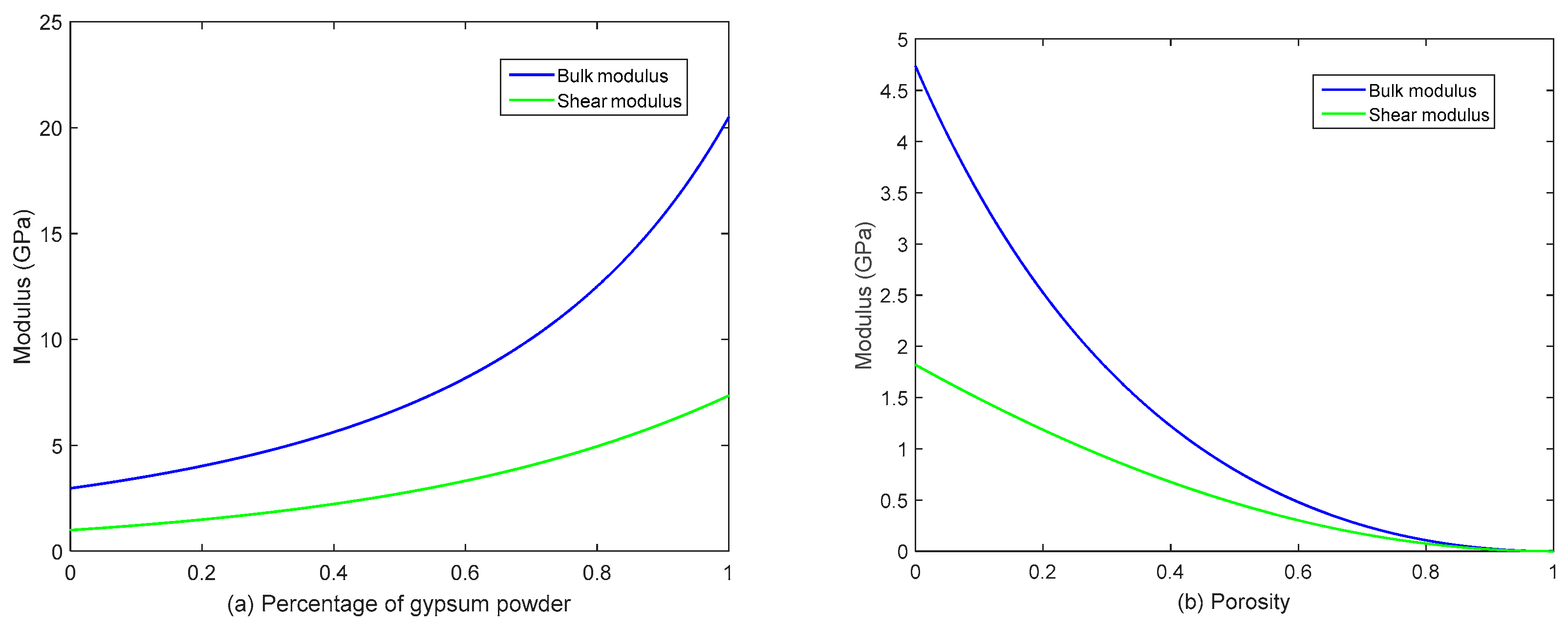
The upscaling process using DEM method is different to the two previous upscaling theories. DEM is done in two separate steps: adding gypsum powder into the binder support as matrix and next, adding the pore space into the solid. The upscaling steps based on this theoretical assumption is demonstrated in Figure 8, where the increase in the amount of gypsum powder and porosity only would take place in theory and truly in physical reality. Figure 8 shows that adding (increase in the percentage) gypsum powder and pore space will alter the modulus values and it can be predicted at each percentage desired based on input parameters into the model. The predicted modulus of four samples were all smaller than M-T and SCS methods (Table 4).
5. Discussion
5.1. The Comparison of Upscaling Methods
First, comparing these three upscaling methods, differential effective medium (DEM) method generates the lowest values of modulus than M-T and SCS methods. Regarding samples vertical 1 and horizontal 1, the M-T method provided us with a lower modulus than the SCS method while the opposite is true for sample vertical 2 and horizontal 2. Most importantly, the prediction of modulus via three different upscaling methods would be insufficient unless these values are with macroscale modulus measured by UCS and Triaxial compression experiments. Young’ s modulus was calculated by determining the tangent modulus at 50% of the peak strength value. Table 5 shows the summarized characteristics of sample size from two measurements in this study, plus six additional ones taken from the literature. Considering this table, the samples 1 and 2 tested in this study showed Young’s modulus values of 0.1967 and 0.3125 GPa, which are extremely low compared to the upscaled modulus values calculated by three different theoretical methods. In order to have a better comparison, another group of 3D printed gypsum samples were selected for further comparison and reference with modulus values in the ranges of 2–5 GPa, measured by UCS experiments [31]. The discrepancy between different groups of 3D printed samples made of gypsum powder owes to two possible reasons. The primary factor is the binder saturation, which is set prior to printing processing. Generally, the manufacturers are prone to save the consumption of materials used, thus the binder saturation is much lower than anticipated value, decreasing the mechanical performance in this study. The samples 5, 6, 7, and 8 used in the study by Fereshtenejad and Song have the binder saturation of 100%, 120%, 135%, and 150%, respectively [31]. Postprocessing effect, infiltration specifically, significantly alters the mechanical property of 3D printed rocks, which, on the other hand, cannot penetrate completely into the samples using the infiltrant (glue). If abundant pore spaces were remained in the central part [80], the modulus of bulk samples could not meet the expectation. Therefore, samples 5–8 that experienced sufficient postprocessing steps with higher binder saturation were selected to be the reference for comparison with the values that were predicted by upscaling methods. It is observed that M-T Scheme and SCS methods exhibited better prediction performance than the DEM method. We would suggest that both of these methods should be utilized when upscaling mechanical properties of multiple composite materials from microscale to macroscale.
5.2. Rock Physics and 3D Printing Technology
The application of 3D printed rocks in rock mechanical experiments leads to a serious of issues which are apparent in the above comparison. A major one is the repeatability in terms of mechanical performance. Sample size is one of the factors that needs to be determined prior to the experiments since the effect that size would have on the results is significant [32]. Using different powder density and binder saturation and various post-processing effects will definitely alter the pore structure, transport and geomechanical properties, that has been discussed in recent studies [31,33,34]. We would suggest keeping the material type and the proportions of them constant, which is possible and controllable in 3D printing, and then try different post-processing procedures to determine the best practice. The most suitable post-processing method is the one that would generate samples with comparable results with upscaled values. For instance, cleaning the samples by air gun and infiltration cannot guarantee the same results and will alter sample structure which will end in samples with varying modulus values.
When the best practice for post-processing and sample preparation is decided, the potential application of 3D printing technology in rock mechanics is to substitute any rock type with 3D printed powder-based samples to investigate fracture mechanism and verify failure modes [85,86,87,88]. A good example is the interaction between natural fractures and induced fractures, which is challenging under laboratory conditions since natural samples taken from subsurface are very complex in nature and constituent components. By taking advantage of similar brittle elastic behavior of powder-based samples through 3D printing, by adding pre-existing fractures to desired directions within the sample, a series of experiments can be developed to validate various numerical simulations to study fracture mechanics. Furthermore, if the additive manufacturing industry can develop a rock-similar material through mixing several minerals that are also major components of most common rock types, to replace the single component printed materials, heterogeneity and anisotropic failures can also be examined more realistically. If the binder can play the similar role as the clay matrix, 3D printed samples will become very similar in performance to natural rocks in regards to microstructure and mechanical properties. The computational models of failure mechanisms in heterogeneous rocks with pre-existing cracks, defects and pores [88] can be precisely validated by designing and manufacturing a series of heterogeneous rocks by 3D printing technology if all conditions above are combined. Though gradual progression towards this goal should be made, it will be a tremendous contribution to the laboratory experiments in geoscience and petroleum engineering.
6. Conclusions
This study attempted to validate the upscaling methods on geomechanical properties that were measured through a combination of nanoindentation experiments and triaxial testing, using 3D printed rocks as a linear elastic material with simple component instead of a rock that has complex constituents. The 3D printed samples that have simple components of gypsum powder and binder, were first tested in nanoindentation experiments to measure Young’s modulus and hardness of each grain/component, and then followed by a deconvolution method to separate the two existing phases in terms of peak value and frequency fractions.
Mori-Tanaka method, self-consistent scheme (SCS) method and different effective medium (DEM) method were examined for their performance for upscaling mechanical properties from microscale to macroscale. Comparing macroscale Young’s modulus of 3D printed rocks that was obtained from M-T and SCS methods demonstrates more comparable values than DEM with macroscale values acquired from triaxial and UCS testing. It is suggested that M-T and SCS methods are used when dealing with upscaling problems related to a linear elastic medium, though more complicated materials with heterogeneity and anisotropy should be further examined for the best upscaling method. Additionally, the application of 3D printing technology in rock mechanics experiments is still very immature, but promising, and should get further attention from various perspectives including developing input materials to the printing and post-processing processes for the most reliable and rock-like samples.
Author Contributions
Data curation, S.Z. and G.G.M.; Formal analysis, L.K.; Funding acquisition, M.O.; Methodology, M.O, S.Z., B.L., G.G.M. and C.L.; Software, C.L.; Validation, B.L.; Writing—original draft, L.K.; Writing—review & editing, M.O.
Funding
This research was supported by the private donation from the Hughes-Fogarty Family Research Fund to the Petroleum Engineering Department at the University of North Dakota (Fund #67441).
Acknowledgments
The author greatly appreciates the American Association of Petroleum Geologists Foundation for awarding the 2017 Grand-in-aid. Co-author, Dr. Bo Liu, is supported by University Nursing Program for Young Scholars with Creative Talents in Heilongjianng Province (UNPYSCT-2015077).
Conflicts of Interest
The authors declare no conflict of interest.
Nomenclature
| Stiffness tensor | |
| C | Stiffness coefficient |
| c | Multi-variate Gaussian normal density |
| E | Young’s modulus |
| Volume fraction | |
| G | Shear modulus |
| hmax | Maximum displacement |
| K | Bulk modulus |
| N | quantity of all components |
| Hill tensor | |
| Probability density function | |
| Pmax | Peak load |
| S | Contact stiffness |
| T | Total parameters |
| Us | Absolute energy |
| Ue | Elastic energy |
| vE | Elastic energy ratio |
| X | Multi-dimensional array |
| Mean matrices of phase j. | |
| Posterior probability | |
| Fractional difference between horizontal () and vertical () P-wave | |
| Fractional difference between horizontally polarized () and vertically polarized () shear wave |
References
- Guo, Y.; Deng, P.; Yang, C.; Chang, X.; Wang, L.; Zhou, J. Experimental Investigation on Hydraulic Fracture Propagation of Carbonate Rocks under Different Fracturing Fluids. Energies 2018, 11, 3502. [Google Scholar] [CrossRef]
- Peng, J.; Yang, S.-Q. Comparison of mechanical behavior and acoustic emission characteristics of three thermally-damaged rocks. Energies 2018, 11, 2350. [Google Scholar] [CrossRef]
- Chang, X.; Guo, Y.; Zhou, J.; Song, X.; Yang, C. Numerical and Experimental Investigations of the Interactions between Hydraulic and Natural Fractures in Shale Formations. Energies 2018, 11, 2541. [Google Scholar] [CrossRef]
- Li, Y.; Liu, C.; Liu, L.; Sun, J.; Liu, H.; Meng, Q. Experimental study on evolution behaviors of triaxial-shearing parameters for hydrate-bearing intermediate fine sediment. Adv. Geo-Energy Res. 2018, 2, 43–52. [Google Scholar] [CrossRef]
- Liu, R.; Jiang, Y.; Huang, N.; Sugimoto, S. Hydraulic properties of 3D crossed rock fractures by considering anisotropic aperture distributions. Adv. Geo-Energy Res. 2018, 2, 113–121. [Google Scholar] [CrossRef]
- Wanniarachchi, A.; Pathegama Gamage, R.; Lyu, Q.; Perera, S.; Wickramarathne, H.; Rathnaweera, T. Mechanical Characterization of Low Permeable Siltstone under Different Reservoir Saturation Conditions: An Experimental Study. Energies 2019, 12, 14. [Google Scholar] [CrossRef]
- Ulm, F.-J.; Abousleiman, Y. The nanogranular nature of shale. Acta Geotech. 2006, 1, 77–88. [Google Scholar] [CrossRef]
- Bobko, C.P. Assessing the Mechanical Microstructure of Shale by Nanoindentation: The Link between Mineral Composition and Mechanical Properties. Ph.D. Thesis, Massachusetts Institute of Technology, Cambridge, MA, USA, 2008. [Google Scholar]
- Deirieh, A.; Ortega, J.; Ulm, F.-J.; Abousleiman, Y. Nanochemomechanical assessment of shale: a coupled WDS-indentation analysis. Acta Geotech. 2012, 7, 271–295. [Google Scholar] [CrossRef]
- Rassouli, F.; Ross, C.; Zoback, M.; Andrew, M. Shale Rock Characterization Using Multi-Scale Imaging. In Proceedings of the 51st US Rock Mechanics/Geomechanics Symposium, San Francisco, CA, USA, 25–28 June 2017. [Google Scholar]
- Dubey, V.; Abedi, S.; Noshadravan, A. Multiscale Modelling of Microcrack-Induced Mechanical Properties in Shales. In Proceedings of the 52nd US Rock Mechanics/Geomechanics Symposium, Seattle, WA, USA, 17–20 June 2018. [Google Scholar]
- Li, C.; Ostadhassan, M.; Guo, S.; Gentzis, T.; Kong, L. Application of PeakForce tapping mode of atomic force microscope to characterize nanomechanical properties of organic matter of the Bakken Shale. Fuel 2018, 233, 894–910. [Google Scholar] [CrossRef]
- Li, C.; Ostadhassan, M.; Gentzis, T.; Kong, L.; Carvajal-Ortiz, H.; Bubach, B. Nanomechanical characterization of organic matter in the Bakken formation by microscopy-based method. Mar. Pet. Geol. 2018, 96, 128–138. [Google Scholar] [CrossRef]
- Li, C.; Ostadhassan, M.; Abarghani, A.; Fogden, A.; Kong, L. Multi-scale evaluation of mechanical properties of the Bakken shale. J. Mater. Sci. 2019, 54, 2133–2151. [Google Scholar] [CrossRef]
- Shukla, P.; Kumar, V.; Curtis, M.; Sondergeld, C.H.; Rai, C.S. Nanoindentation studies on shales. In Proceedings of the 47th US Rock Mechanics/Geomechanics Symposium, San Francisco, CA, USA, 23–26 June 2013. [Google Scholar]
- Mighani, S.; Taneja, S.; Sondergeld, C.; Rai, C. Nanoindentation creep measurements on shale. In Proceedings of the 49th US Rock Mechanics/Geomechanics Symposium, San Francisco, CA, USA, 28 June–1 July 2015. [Google Scholar]
- Vialle, S.; Lebedev, M. Heterogeneities in the elastic properties of microporous carbonate rocks at the microscale from nanoindentation tests. In SEG Technical Program Expanded Abstracts 2015; Society of Exploration Geophysicists: Tulsa, OK, USA, 2015; pp. 3279–3284. [Google Scholar]
- Françis, D.; Pineau, A.; Zaoui, A. Mechanical Behaviour of Materials; Kluwer academic publishers: Dordrecht, The Netherlands, 1988. [Google Scholar]
- Constantinides, G.; Ulm, F.-J. The effect of two types of CSH on the elasticity of cement-based materials: Results from nanoindentation and micromechanical modeling. Cement Concr. Res. 2004, 34, 67–80. [Google Scholar] [CrossRef]
- Levin, V.; Markov, M.; Kanaun, S. Effective field method for seismic properties of cracked rocks. J. Geophys. Res. Solid Earth 2004, 109. [Google Scholar] [CrossRef]
- Nguyen, N.; Giraud, A.; Grgic, D. A composite sphere assemblage model for porous oolitic rocks. Int. J. Rock Mech. Min. Sci. 2011, 48, 909–921. [Google Scholar] [CrossRef]
- Peng, J.; Rong, G.; Cai, M.; Zhou, C.-B. A model for characterizing crack closure effect of rocks. Eng. Geol. 2015, 189, 48–57. [Google Scholar] [CrossRef]
- Zhu, Q.; Shao, J.-F. A refined micromechanical damage–friction model with strength prediction for rock-like materials under compression. Int. J. Solids Struct. 2015, 60, 75–83. [Google Scholar] [CrossRef]
- Campbell, T.; Williams, C.; Ivanova, O.; Garrett, B. Could 3D printing change the world. In Technologies, Potential, and Implications of Additive Manufacturing; Atlantic Council: Washington, DC, USA, 2011. [Google Scholar]
- Espalin, D.; Muse, D.W.; MacDonald, E.; Wicker, R.B. 3D Printing multifunctionality: structures with electronics. Int. J. Adv. Manuf. Technol. 2014, 72, 963–978. [Google Scholar] [CrossRef]
- Mitsouras, D.; Liacouras, P.; Imanzadeh, A.; Giannopoulos, A.A.; Cai, T.; Kumamaru, K.K.; George, E.; Wake, N.; Caterson, E.J.; Pomahac, B.; et al. Medical 3D printing for the radiologist. Radiographics 2015, 35, 1965–1988. [Google Scholar] [CrossRef]
- Chia, H.N.; Wu, B.M. Recent advances in 3D printing of biomaterials. J. Biol. Eng. 2015, 9, 4. [Google Scholar] [CrossRef]
- Mozafari, H.; Dong, P.; Hadidi, H.; Sealy, M.; Gu, L. Mechanical Characterizations of 3D-printed PLLA/Steel Particle Composites. Materials 2019, 12, 1. [Google Scholar] [CrossRef]
- Ishutov, S.; Jobe, T.D.; Zhang, S.; Gonzalez, M.; Agar, S.M.; Hasiuk, F.J.; Watson, F.; Geiger, S.; Mackay, E.; Chalaturnyk, R. Three-dimensional printing for geoscience: Fundamental research, education, and applications for the petroleum industry. AAPG Bull. 2018, 102, 1–26. [Google Scholar] [CrossRef]
- Jiang, C.; Zhao, G.-F.; Zhu, J.; Zhao, Y.-X.; Shen, L. Investigation of dynamic crack coalescence using a gypsum-like 3D printing material. Rock Mech. Rock Eng. 2016, 49, 3983–3998. [Google Scholar] [CrossRef]
- Fereshtenejad, S.; Song, J.-J. Fundamental study on applicability of powder-based 3D printer for physical modeling in rock mechanics. Rock Mech. Rock Eng. 2016, 49, 2065–2074. [Google Scholar] [CrossRef]
- Kong, L.; Ostadhassan, M.; Li, C.; Tamimi, N. Can 3-D Printed Gypsum Samples Replicate Natural Rocks? An Experimental Study. Rock Mech. Rock Eng. 2018, 51, 3061–3074. [Google Scholar] [CrossRef]
- Primkulov, B.; Chalaturnyk, J.; Chalaturnyk, R.; Zambrano Narvaez, G. 3D Printed Sandstone Strength: Curing of Furfuryl Alcohol Resin-Based Sandstones. 3D Print. Addit. Manuf. 2017, 4, 149–156. [Google Scholar] [CrossRef]
- Kong, L.; Ostadhassan, M.; Liu, B.; Li, C.; Liu, K. Multifractal Characteristics of MIP-Based Pore Size Distribution of 3D-Printed Powder-Based Rocks: A Study of Post-Processing Effect. Transp. Porous Media 2018. [Google Scholar] [CrossRef]
- Hainsworth, S.; Page, T. Nanoindentation studies of the chemomechanical effect in sapphire. J. Mater. Sci. 1994, 29, 5529–5540. [Google Scholar] [CrossRef]
- Wilkinson, T.M.; Zargari, S.; Prasad, M.; Packard, C.E. Optimizing nano-dynamic mechanical analysis for high-resolution, elastic modulus mapping in organic-rich shales. J. Mater. Sci. 2015, 50, 1041–1049. [Google Scholar] [CrossRef]
- Rohbeck, N.; Tsivoulas, D.; Shapiro, I.P.; Xiao, P.; Knol, S.; Escleine, J.-M.; Perez, M.; Liu, B. Comparison study of silicon carbide coatings produced at different deposition conditions with use of high temperature nanoindentation. J. Mater. Sci. 2017, 52, 1868–1882. [Google Scholar] [CrossRef]
- Jha, K.K.; Suksawang, N.; Lahiri, D.; Agarwal, A. Energy-Based Analysis of Nanoindentation Curves for Cementitious Materials. ACI Mater. J. 2012, 109. [Google Scholar]
- Vandamme, M.; Ulm, F.-J. Nanogranular origin of concrete creep. Proc. Natl. Acad. Sci. USA 2009, 106, 10552–10557. [Google Scholar] [CrossRef] [PubMed]
- Liu, K.; Ostadhassan, M.; Xu, X.; Bubach, B. Abnormal behavior during nanoindentation holding stage: Characterization and explanation. J. Pet. Sci. Eng. 2019, 173, 733–747. [Google Scholar] [CrossRef]
- Cheng, Y.-T.; Cheng, C.-M. Scaling approach to conical indentation in elastic-plastic solids with work hardening. J. Appl. Phys. 1998, 84, 1284–1291. [Google Scholar] [CrossRef]
- Jha, K.K.; Suksawang, N.; Lahiri, D.; Agarwal, A. A novel energy-based method to evaluate indentation modulus and hardness of cementitious materials from nanoindentation load–displacement data. Mater. Struct. 2015, 48, 2915–2927. [Google Scholar] [CrossRef]
- Oliver, W.C.; Pharr, G.M. An improved technique for determining hardness and elastic modulus using load and displacement sensing indentation experiments. J. Mater. Res. 1992, 7, 1564–1583. [Google Scholar] [CrossRef]
- Dempster, A.P.; Laird, N.M.; Rubin, D.B. Maximum likelihood from incomplete data via the EM algorithm. J. R. Stat. Soc. Ser. B 1977, 39, 1–38. [Google Scholar] [CrossRef]
- McLachlan, G.J.; Basford, K.E. Mixture Models: Inference and Applications to Clustering; Marcel Dekker: New York, NY, USA, 1988; Volume 84. [Google Scholar]
- Moon, T.K. The expectation-maximization algorithm. IEEE Signal Process. Mag. 1996, 13, 47–60. [Google Scholar] [CrossRef]
- Bhat, H.S.; Kumar, N. On the Derivation of the Bayesian Information Criterion; School of Natural Sciences, University of California: Oakland, CA, USA, 2010. [Google Scholar]
- Schwarz, G. Estimating the dimension of a model. Ann. Stat. 1978, 6, 461–464. [Google Scholar] [CrossRef]
- Yang, K.-H.; Yalew, W.M.; Nguyen, M.D. Behavior of geotextile-reinforced clay with a coarse material sandwich technique under unconsolidated-undrained triaxial compression. Int. J. Geomech. 2015, 16, 04015083. [Google Scholar] [CrossRef]
- Hunsche, U. Uniaxial and triaxial creep and failure tests on rock: experimental technique and interpretation. In Visco-Plastic Behaviour of Geomaterials; Springer: Vienna, Austria, 1994; pp. 1–53. [Google Scholar]
- Chen, Y.; Joffre, D.; Avitabile, P. Underwater Dynamic Response at Limited Points Expanded to Full-Field Strain Response. J. Vib. Acoust. 2018, 140, 051016. [Google Scholar] [CrossRef]
- Fjar, E.; Holt, R.M.; Raaen, A.; Risnes, R.; Horsrud, P. Petroleum Related Rock Mechanics; Elsevier: Amsterdam, The Netherlands, 2008; Volume 53. [Google Scholar]
- Mukerji, T.; Berryman, J.; Mavko, G.; Berge, P. Differential effective medium modeling of rock elastic moduli with critical porosity constraints. Geophys. Res. Lett. 1995, 22, 555–558. [Google Scholar] [CrossRef]
- Berryman, J.G. Effective medium theories for multicomponent poroelastic composites. J. Eng. Mech. 2006, 132, 519–531. [Google Scholar] [CrossRef]
- Choy, T.C. Effective Medium Theory: Principles and Applications; Oxford University Press: Oxford, UK, 2015; Volume 165. [Google Scholar]
- Hashin, Z.; Shtrikman, S. A variational approach to the theory of the elastic behaviour of multiphase materials. J. Mech. Phys. Solids 1963, 11, 127–140. [Google Scholar] [CrossRef]
- Benveniste, Y. A new approach to the application of Mori-Tanaka’s theory in composite materials. Mech. Mater. 1987, 6, 147–157. [Google Scholar] [CrossRef]
- Miled, K.; Sab, K.; Le Roy, R. Effective elastic properties of porous materials: Homogenization schemes vs experimental data. Mech. Res. Commun. 2011, 38, 131–135. [Google Scholar] [CrossRef]
- Giraud, A.; Nguyen, N.; Grgic, D. Effective poroelastic coefficients of isotropic oolitic rocks with micro and meso porosities. Int. J. Eng. Sci. 2012, 58, 57–77. [Google Scholar] [CrossRef]
- Gercek, H. Poisson’s ratio values for rocks. Int. J. Rock Mech. Min. Sci. 2007, 44, 1–13. [Google Scholar] [CrossRef]
- Berryman, J.G. Mixture theories for rock properties. Rock Phys. Phase Relat. Handb. Phys. Constants 1995, 3, 205–228. [Google Scholar]
- Mavko, G.; Mukerji, T.; Dvorkin, J. The Rock Physics Handbook: Tools for Seismic Analysis of Porous Media; Cambridge University Press: Cambridge, UK, 2009. [Google Scholar]
- Berryman, J.G. Long-wavelength propagation in composite elastic media II. Ellipsoidal inclusions. J. Acoust. Soc. Am. 1980, 68, 1820–1831. [Google Scholar] [CrossRef]
- Dey, A.; Mukhopadhyay, A.K. Nanoindentation of Brittle Solids; CRC Press: Boca Raton, FL, USA, 2014. [Google Scholar]
- Kong, L.; Ostadhassan, M.; Li, C.; Tamimi, N. Pore characterization of 3D-printed gypsum rocks: A comprehensive approach. J. Mater. Sci. 2018, 53, 5063–5078. [Google Scholar] [CrossRef]
- Tavallali, A.; Vervoort, A. Failure of layered sandstone under Brazilian test conditions: effect of micro-scale parameters on macro-scale behaviour. Rock Mech. Rock Eng. 2010, 43, 641–653. [Google Scholar] [CrossRef]
- Dutta, P.; Mavko, G. Effect of micro-scale anisotropy on solid substitution in macro-scale isotropic composites. In Proceedings of the 2015 SEG Annual Meeting, New Orleans, LA, USA, 18–23 October 2015. [Google Scholar]
- Sharfeddin, A.; Volinsky, A.A.; Mohan, G.; Gallant, N.D. Comparison of the macroscale and microscale tests for measuring elastic properties of polydimethylsiloxane. J. Appl. Polym. Sci. 2015, 132. [Google Scholar] [CrossRef]
- Keller, L.M.; Schwiedrzik, J.J.; Gasser, P.; Michler, J. Understanding Anisotropic Mechanical Properties of Shales at Different Length Scales: In-Situ Micropillar Compression Combined with Finite Element Calculations. J. Geophys. Res. Solid Earth 2017, 122, 5945–5955. [Google Scholar] [CrossRef]
- Zhang, Y.; Lebedev, M.; Al-Yaseri, A.; Yu, H.; Xu, X.; Iglauer, S. Characterization of nanoscale rockmechanical properties and microstructures of a Chinese sub-bituminous coal. J. Nat. Gas Sci. Eng. 2018, 52, 106–116. [Google Scholar] [CrossRef]
- Yang, H.; Luo, S.; Zhang, G.; Song, J. Elasticity of Clay Shale Characterized by Nanoindentation. In Proceedings of the 51st US Rock Mechanics/Geomechanics Symposium, San Francisco, CA, USA, 25–28 June 2017. [Google Scholar]
- Sanahuja, J.; Dormieux, L.; Meille, S.; Hellmich, C.; Fritsch, A. Micromechanical explanation of elasticity and strength of gypsum: from elongated anisotropic crystals to isotropic porous polycrystals. J. Eng. Mech. 2009, 136, 239–253. [Google Scholar] [CrossRef]
- Coon, C.; Pretzel, B.; Lomax, T.; Strlič, M. Preserving rapid prototypes: A review. Herit. Sci. 2016, 4, 40. [Google Scholar] [CrossRef]
- Gardan, J. Method for characterization and enhancement of 3D printing by binder jetting applied to the textures quality. Assem. Autom. 2017, 37, 162–169. [Google Scholar] [CrossRef]
- Dowling, N.E. Mechanical Behavior of Materials; Pearson: London, UK, 2012. [Google Scholar]
- Amann, F.; Kaiser, P.; Button, E.A. Experimental study of brittle behavior of clay shale in rapid triaxial compression. Rock Mech. Rock Eng. 2012, 45, 21–33. [Google Scholar] [CrossRef]
- Yang, S.-Q.; Jing, H.-W.; Wang, S.-Y. Experimental investigation on the strength, deformability, failure behavior and acoustic emission locations of red sandstone under triaxial compression. Rock Mech. Rock Eng. 2012, 45, 583–606. [Google Scholar] [CrossRef]
- Yoneda, J.; Masui, A.; Konno, Y.; Jin, Y.; Egawa, K.; Kida, M.; Ito, T.; Nagao, J.; Tenma, N. Mechanical behavior of hydrate-bearing pressure-core sediments visualized under triaxial compression. Mar. Pet. Geol. 2015, 66, 451–459. [Google Scholar] [CrossRef]
- Goodman, R.E. Introduction to Rock Mechanics; Wiley: New York, NY, USA, 1989; Volume 2. [Google Scholar]
- Ishutov, S.; Hasiuk, F.J.; Fullmer, S.M.; Buono, A.S.; Gray, J.N.; Harding, C. Resurrection of a reservoir sandstone from tomographic data using three-dimensional printing. AAPG Bull. 2017, 101, 1425–1443. [Google Scholar] [CrossRef]
- Wei, Q.; Wang, Y.; Chai, W.; Zhang, Y.; Chen, X. Molecular dynamics simulation and experimental study of the bonding properties of polymer binders in 3D powder printed hydroxyapatite bioceramic bone scaffolds. Ceram. Int. 2017, 43, 13702–13709. [Google Scholar] [CrossRef]
- Higgins, S.M.; Goodwin, S.A.; Bratton, T.R.; Tracy, G.W. Anisotropic stress models improve completion design in the Baxter Shale. In Proceedings of the SPE Annual Technical Conference and Exhibition, Denver, CO, USA, 21–24 September 2008. [Google Scholar]
- Thomsen, L. Weak elastic anisotropy. Geophysics 1986, 51, 1954–1966. [Google Scholar] [CrossRef]
- Ostadhassan, M.; Zeng, Z.; Jabbari, H. Anisotropy analysis in shale using advanced sonic data-Bakken Case Study. In Proceedings of the American Association of Petroleum Geologists (AAPG) Annual Convention, Long Beach, CA, USA, 22–25 April 2012. [Google Scholar]
- Scholtès, L.; Donzé, F.-V. Modelling progressive failure in fractured rock masses using a 3D discrete element method. Int. J. Rock Mech. Min. Sci. 2012, 52, 18–30. [Google Scholar] [CrossRef]
- Mahabadi, O.K.; Lisjak, A.; Munjiza, A.; Grasselli, G. Y-Geo: New combined finite-discrete element numerical code for geomechanical applications. Int. J. Geomech. 2012, 12, 676–688. [Google Scholar] [CrossRef]
- Nikolic, M.; Ibrahimbegovic, A. Rock mechanics model capable of representing initial heterogeneities and full set of 3D failure mechanisms. Comput. Methods Appl. Mech. Eng. 2015, 290, 209–227. [Google Scholar] [CrossRef]
- Nikolic, M.; Ibrahimbegovic, A.; Miscevic, P. Brittle and ductile failure of rocks: embedded discontinuity approach for representing mode I and mode II failure mechanisms. Int. J. Numer. Methods Eng. 2015, 102, 1507–1526. [Google Scholar] [CrossRef]
Figure 1.
Surface model representing 3D printed cylindrical samples 1 and 2.

Figure 2.
3D printed rock fragments for nanoindentation experiments. ‘V’ represents vertical, and ‘H’ denotes horizontal.
Figure 2.
3D printed rock fragments for nanoindentation experiments. ‘V’ represents vertical, and ‘H’ denotes horizontal.

Figure 3.
Typical load-displacement curve in a nanoindentation test (E represents Young’s modulus) (modified from Jha et al. [38]).
Figure 3.
Typical load-displacement curve in a nanoindentation test (E represents Young’s modulus) (modified from Jha et al. [38]).
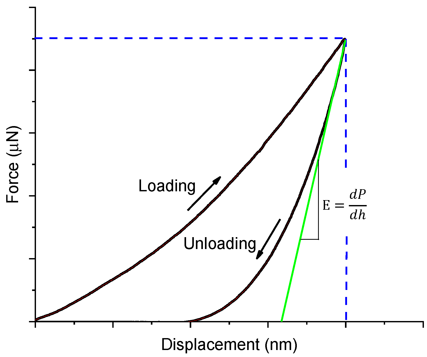
Figure 4.
Statistical analysis (box plot) of Young’s modulus of four samples where vertical and horizontal corresponds to the mode of printing (depositing particles by the printer).
Figure 4.
Statistical analysis (box plot) of Young’s modulus of four samples where vertical and horizontal corresponds to the mode of printing (depositing particles by the printer).

Figure 5.
Relationship between Young’s modulus and hardness of four samples.

Figure 6.
Stress–strain curve of 3D printed rock (a) cylindrical sample 1 and (b) cylindrical sample 2 made of gypsum-powder.
Figure 6.
Stress–strain curve of 3D printed rock (a) cylindrical sample 1 and (b) cylindrical sample 2 made of gypsum-powder.

Figure 7.
Failure envelope and Mohr’s circles of 3D printed rocks made up of gypsum powder. Cohesion (C) is 0.68 MPa and internal friction angle () is 41°.
Figure 7.
Failure envelope and Mohr’s circles of 3D printed rocks made up of gypsum powder. Cohesion (C) is 0.68 MPa and internal friction angle () is 41°.

Figure 8.
Upscaling of modulus at macroscale for representative sample vertical 1.

Table 1.
Deconvolution results of Young’s modulus of four samples.
| Sample ID | Phase | Probability | Mean Young’s Modulus (GPa) | Standard Deviation (GPa) |
|---|---|---|---|---|
| V1 | binder | 0.70 | 2.67 | 1.14 |
| gypsum | 0.30 | 19.68 | 16.48 | |
| H1 | binder | 0.73 | 3.39 | 1.77 |
| gypsum | 0.27 | 39.36 | 17.29 | |
| V2 | binder | 0.73 | 5.86 | 2.30 |
| gypsum | 0.27 | 24.06 | 12.73 | |
| H2 | binder | 0.77 | 3.36 | 0.95 |
| gypsum | 0.23 | 8.27 | 4.23 |
Table 2.
Upscaling results of four samples using the Mori-Tanaka (M-T) method.
| Sample | Gypsum (%) | Binder (%) | Porosity | Young’s Modulus (GPa) | ||
|---|---|---|---|---|---|---|
| Vertical 1 | 0.20 | 0.48 | 0.32 | 2.74 | 1.05 | –0.03 |
| Horizontal 1 | 0.18 | 0.50 | 0.32 | 3.54 | 1.08 | –0.03 |
| Vertical 2 | 0.18 | 0.50 | 0.32 | 5.19 | 1.98 | –0.02 |
| Horizontal 2 | 0.16 | 0.52 | 0.32 | 2.57 | 0.73 | –0.01 |
Table 3.
Upscaling results of four samples using self-consistent scheme (SCS) method.
| Sample | Gypsum (%) | Binder (%) | Porosity | Young’s Modulus (GPa) | ||
|---|---|---|---|---|---|---|
| Vertical 1 | 0.20 | 0.48 | 0.32 | 2.81 | 0.86 | –0.02 |
| Horizontal 1 | 0.18 | 0.50 | 0.32 | 3.67 | 1.16 | –0.03 |
| Vertical 2 | 0.18 | 0.50 | 0.32 | 4.98 | 0.80 | –0.02 |
| Horizontal 2 | 0.16 | 0.52 | 0.32 | 2.40 | 0.77 | –0.01 |
Table 4.
Upscaling results of four samples using differential effective medium theory.
| Sample | Porosity for Upscaling (Dimensionless) | Bulk Modulus (GPa) | Shear Modulus (GPa) | Young’s Modulus (GPa) |
|---|---|---|---|---|
| Vertical 1 | 0.32 | 1.66 | 0.86 | 1.49 |
| Horizontal 1 | 0.32 | 2.22 | 1.17 | 2.00 |
| Vertical 2 | 0.32 | 3.01 | 1.52 | 2.71 |
| Horizontal 2 | 0.32 | 1.48 | 0.73 | 1.33 |
Table 5.
Macroscale Young’s modulus of 3D printed gypsum samples by Uniaxial Compression Strength (UCS) and triaxial experiments.
Table 5.
Macroscale Young’s modulus of 3D printed gypsum samples by Uniaxial Compression Strength (UCS) and triaxial experiments.
| Cylindrical Sample * | Length (mm) | Diameter (mm) | Young’s Modulus (Gpa) |
|---|---|---|---|
| 1 | 89 | 36 | 0.20 |
| 2 | 89 | 36 | 0.31 |
| 3 | 120 | 50 | 0.32 |
| 4 | 60 | 25 | 0.75 |
| 5 | 100 | 50 | 2.39 |
| 6 | 100 | 50 | 2.43 |
| 7 | 100 | 50 | 3.62 |
| 8 | 100 | 50 | 4.59 |
© 2019 by the authors. Licensee MDPI, Basel, Switzerland. This article is an open access article distributed under the terms and conditions of the Creative Commons Attribution (CC BY) license (http://creativecommons.org/licenses/by/4.0/).
Share and Cite
MDPI and ACS Style
Kong, L.; Ostadhassan, M.; Zamiran, S.; Liu, B.; Li, C.; Marino, G.G. Geomechanical Upscaling Methods: Comparison and Verification via 3D Printing. Energies 2019, 12, 382. https://doi.org/10.3390/en12030382
AMA Style
Kong L, Ostadhassan M, Zamiran S, Liu B, Li C, Marino GG. Geomechanical Upscaling Methods: Comparison and Verification via 3D Printing. Energies. 2019; 12(3):382. https://doi.org/10.3390/en12030382
Chicago/Turabian StyleKong, Lingyun, Mehdi Ostadhassan, Siavash Zamiran, Bo Liu, Chunxiao Li, and Gennaro G. Marino. 2019. "Geomechanical Upscaling Methods: Comparison and Verification via 3D Printing" Energies 12, no. 3: 382. https://doi.org/10.3390/en12030382
Note that from the first issue of 2016, this journal uses article numbers instead of page numbers. See further details here.