Stochastic Planning of Distributed PV Generation


1
Department of Electrical & Computer Engineering, The University of Texas at San Antonio, San Antonio, TX 78249, USA
2
E*TRADE, Arlington, VA 22203, USA
3
San Antonio Water System, San Antonio, TX 78212, USA
*
Author to whom correspondence should be addressed.
Energies 2019, 12(3), 459; https://doi.org/10.3390/en12030459
Submission received: 11 January 2019
/
Revised: 23 January 2019
/
Accepted: 28 January 2019
/
Published: 31 January 2019
(This article belongs to the Special Issue 10 Years Energies - Horizon 2028)
Abstract
:Recent studies by electric utility companies indicate that maximum benefits of distributed solar photovoltaic (PV) units can be reaped when siting and sizing of PV systems is optimized. This paper develops a two-stage stochastic program that serves as a tool for optimally determining the placing and sizing of PV units in distribution systems. The PV model incorporates the mapping from solar irradiance to AC power injection. By modeling the uncertainty of solar irradiance and loads by a finite set of scenarios, the goal is to achieve minimum installation and network operation costs while satisfying necessary operational constraints. First-stage decisions are scenario-independent and include binary variables that represent the existence of PV units, the area of the PV panel, and the apparent power capability of the inverter. Second-stage decisions are scenario-dependent and entail reactive power support from PV inverters, real and reactive power flows, and nodal voltages. Optimization constraints account for inverter’s capacity, PV module area limits, the power flow equations, as well as voltage regulation. A comparison between two designs, one where the DC:AC ratio is pre-specified, and the other where the maximum DC:AC ratio is specified based on historical data, is carried out. It turns out that the latter design reduces costs and allows further reduction of the panel area. The applicability and efficiency of the proposed formulation are numerically demonstrated on the IEEE 34-node feeder, while the output power of PV systems is modeled using the publicly available PVWatts software developed by the National Renewable Energy Laboratory. The overall framework developed in this paper can guide electric utility companies in identifying optimal locations for PV placement and sizing, assist with targeting customers with appropriate incentives, and encourage solar adoption.
1. Introduction
1.1. Motivation and Context
Savings on fuel costs, deferred construction of future power plants, less frequent transmission and distribution upgrades, smaller peak loads, and, subsequently, reduced rate payments to the region interconnection are but a handful of promising prospects of grid-connected distributed photovoltaics (PVs) for electric utility companies [1]. Reinforced by tax incentives, government-mandated renewable portfolio standards, customer-supported initiatives, and consistently decreasing solar generation costs [2], utilities are undergoing ever-increasing deployments of distributed PVs into their electricity grid; especially at the distribution level. For example, in San Antonio, TX, USA, the local utility company accepts applications from residents to lease their rooftops for the purpose of PV installation [3].
Analyses from utilities, however, suggest that the aforementioned advantages of distributed grid-connected PVs on the distribution system can only be practically realized when utilities are strategically involved with PV planning, especially, PV placement and sizing. For instance, Reference [1] points out that investments in distribution lines and substations can be avoided if PVs are installed in a concentrated growing load area. It is further suggested that optimal placement and sizing can help reduce land footprints and prevent associated negative environmental impacts. Another utility study [4] reveals that reduction in distribution line losses can only be achieved by targeted PV installation at specific locations. Involving the distribution system operator in such planning studies has also been encouraged in [5] to increase utility profits by optimal placement of distributed generators, and in [6] to elevate PV hosting capacity of microgrids while reducing network-related overvoltages. The work in [7] points out that installation of PV systems is motivated by distribution grid efficiency mandates and goes on to explore the financial perspectives of utilities and customers in determining optimal PV locations and sizes.
Such evidence has prompted recent utility-level efforts for technical investigations into deployment of PVs at optimal locations so that their grid benefits are maximized [8]. Utilities can use these studies to identify locations and appropriately target customers by providing incentives for solar adoption and by enhancing solar partnership programs such as the “lease-your-rooftop” program in San Antonio. This paper develops an analytical tool that can assist utilities with determining optimal locations and sizes for distributed PVs.
The intermittent nature of solar irradiance further complicates utility’s operations in distribution networks with distributed PV deployments. For instance, mitigating the adverse effects of high solar generation, such as thermal loss incurred by reversal of power flows, must be incorporated in utility services. In addition, solar irradiance uncertainty compromises voltage security [9] by unexpectedly elevating or demoting voltages, leading to potential damages to voltage regulating devices, or even user generation equipment itself [4]. Such technical challenges compound the need for analytical models of PV units that capture the relationship between solar irradiance and PV injection while allowing for seamless integration into system-level studies.
To accommodate such a need, this paper proposes a two-stage stochastic optimization model for optimal placement and sizing of distributed PV units in distribution networks. The objective of the optimal placement and sizing problem is to minimize system installation costs as well as costs incurred by thermal loss while accounting for the uncertainty of PV units and consumer loads. The paper develops an analytical model for PV units that is suitable for system-level studies and is inspired by PVWatts—an off-the-shelf estimator software for PV installations [10,11] produced by the National Renewable Energy Laboratory (NREL). The proposed methodology is intended to serve as a tool for utilities, so that, through optimal placement and sizing, potential benefits of a distributed PV integration into the grid can be realized.
1.2. Literature Review
The problem of sizing and placement of distributed generation (DG) units has been the subject of extensive study; see, e.g., [12,13,14,15] for reviews focusing on various aspects. Recent trends tackle this problem in three major ways: (1) approximate procedures; (2) heuristic or metaheuristic approaches; and (3) mixed-integer programming (MIP) techniques. Examples of each group are reviewed next.
Approximate procedures [16,17] are fast but are mostly pursued to gain insights on simpler problems that assume a single or limited numbers of DG units. As an example, for a maximum number of allocated DG installations, Reference [16] sequentially cites DGs whose capacities are computed according to an analytical formula derived from the minimizers of approximating expressions for real and reactive power loss, around a base-case profile. The distribution network nodes are ranked based on the voltage deviation in the absense of DG, and this information is used to sequentially place DG units in [18].
Heuristic and metaheuristic methods facilitate obtaining reasonably working solutions to very complex NP-hard problems albeit with no guarantees on optimality. A sensitivity-based guided search algorithm is proposed in [5] to assist the particle swarm optimization (PSO) algorithm in solving a joint DG allocation and distribution reconfiguration problem. DG placement and sizing in radial distribution networks to minimize power losses and voltage deviation in the presence of voltage-dependent loads is attained by [19] via the Shuffled Bat algorithm. Support vector machines are used in conjunction with the PSO algorithm in [20] to tackle a chance constrained formulation of the PV placement and sizing problem with a detailed PV model and nonlinear power flows. Loss sensitivity factors are used in [21] to determine DG locations and initial capacities for wind and PV technologies. Antlion optimization is then employed to update DG capacities so as to achieve voltage stability as well as reduced costs associated with DG investment and line thermal loss. Voltage stability is also considered in [22] but optimization is carried out via an improved genetic algorithm. The hybrid artificial bee colony and cuckoo search of [23] is shown to outperform PSO and genetic algorithm variants for DG placement and sizing. Stochastic PV generation scenarios are introduced in the multi-objective PSO algorithm of [24] assuming that solar irradiance follows the beta distribution, but no reactive support is provided by the PV units. Reactive power support based on a constant power factor is introduced in [25].
Comparison between MIP methods and the genetic algorithm in [26] reveals that MIP methods yield improved solutions at the expense of a longer computation time. Mixed-integer linear programming (MILP) is pursued in [27] for robust placement and sizing of dispatchable and intermittent DGs where a set of polyhedral constraints model the uncertainty in wind, PV, and loads. By modeling uncertainty as a set of scenarios, optimal placement and sizing for conservation voltage reduction is tackled in [28]. These works do not consider PV units with reactive power capabilities and consider a simplified linear mapping from solar irradiance to the AC output of the PV units.
Optimal placement and sizing of voltage-source inverter-based PV solar farms and natural gas-based micro-turbines is presented in [29] as a mixed-integer second-order cone program (MISOCP) by leveraging the conic relaxation of power flow equations. The objective is to minimize costs of investment, operation, and emission. Fast reactive power support from the PVs is also accounted for in the planning stage via incorporating a Jacobian-based voltage stability index weighted by the rated PV size. Multistage stochastic programming for optimal placement, sizing, as well as the dispatch of DGs and storage systems is presented in [30] where novel linearized flow-based loss models are exploited to arrive at a MILP formulation. These works consider a generic piecewise relationship between irradiance and PV output where the DC:AC ratio of the inverter has been abstracted within the mapping.
A more detailed system level model that accounts for DC:AC size and the PV module area is given in [31,32], where, to obtain tractable formulations for unbalanced distribution networks, binary placement variables are assumed continuous and semidefinite relaxations or linearizations of the power flow equations are employed. A slightly more detailed model that accommodates a fixed DC:AC ratio as well as the dependencies of AC power output on the module temperature is also presented in [20]. On the other hand, the works in [20,31,32] do not account for the clipping effect of the PV unit, which pertains to the PV inverter limiting the AC power output under high solar irradiance conditions. The clipping effect is accommodated in [25], but the design is limited to optimizing only the active power rating of the PV unit as a consequence of considering only constant-power-factor reactive power support.
1.3. Contributions and Paper Organization
This paper formulates a two-stage stochastic MISOCP formulation for the placement and sizing of distributed PV units in distribution networks. The first stage attends to decisions made during a utility’s planning phase for PV installation, that is, decisions regarding the location and sizing of PV units that minimize installation costs. The second stage captures a utility’s operational phase in terms of costs associated with thermal loss and efforts pertaining to voltage maintenance. Since the first-stage decisions subsequently affect the performance during the second stage, both stages must be solved concurrently. The stochasticity of PV injections and loads is characterized by a finite set of scenarios; for the PV injections in particular, we used solar irradiance data from the PVWatts calculator. The objective is to minimize the installation costs of the PV system as well as the expected value of thermal loss. Two-stage stochastic programming has successfully been used in other aspects of power system planning [33], and this paper demonstrates its effectiveness for the problem at hand. In contrast to the prior art of Section 1.2 and our previous work [32,34,35], the main contributions of this work are as follows:
- In line with standard practice based on the PVWatts calculator, an analytical model for PV units is presented that rigorously maps solar irradiance to the injected AC power. It is shown that the analytical model is nonconvex. Two engineering designs are then offered to bypass the non-convexity.
- Based on realistic data, several homes are considered per node of the distribution network. Together with linearized network equations that adequately describe the relationships between powers and voltages of the distribution network, the developed framework is intended as a tool for utility-level studies.
- Extensive numerical studies on the IEEE 34-bus distribution feeder are carried out. It is shown that the degree of freedom between DC and AC sizes can be leveraged to lower installation costs through reduction of the panel area, in comparison to a scheme where the DC and AC sizes are restricted to conform to a known DC:AC ratio.
2. Network Model and the Optimization Problem
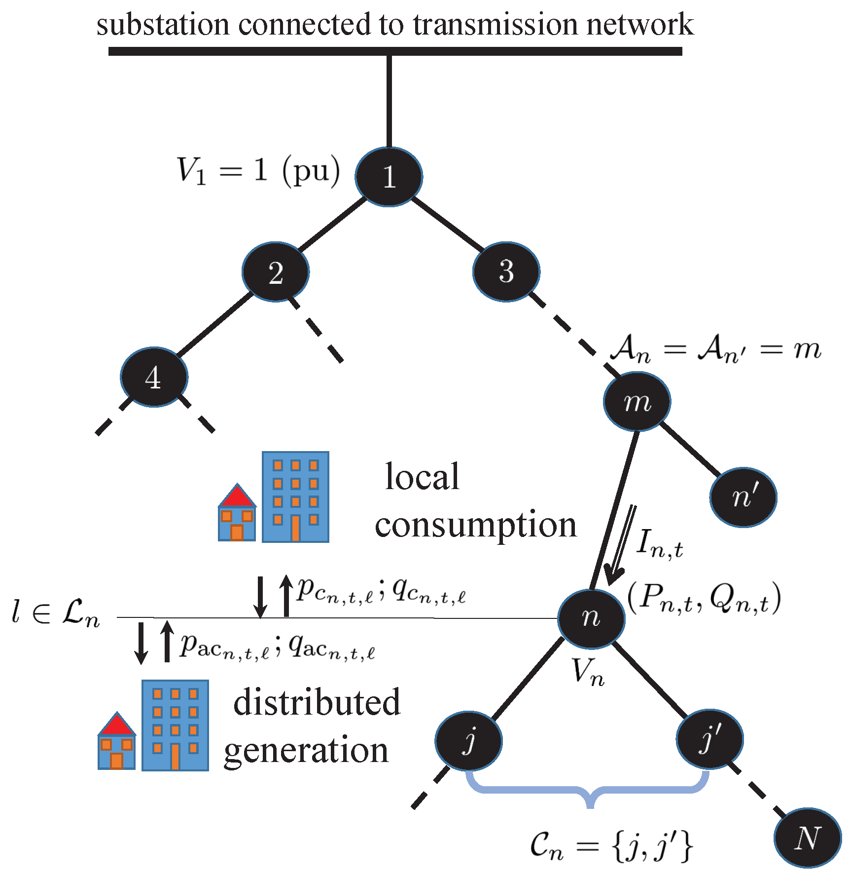
A radial distribution network with a substation and user nodes can be modeled by a tree graph as depicted in Figure 1. Let denote the set of all nodes. The root node is labeled as node 1 and represents the substation connected to the transmission network. The remaining nodes represent user nodes of the distribution network. Every user node has a unique ancestor denoted by . The line connecting node to node n is referred to as line n. A line is referred to by its end node since in a tree network there are no meshes. Moreover, every node has a set of children nodes denoted by .
For example, in Figure 1, the ancestor of node n is and the set of children for node n is . For terminal nodes of the network, is an empty set. Each user node will serve individual homes represented by .
2.1. PV Module Model
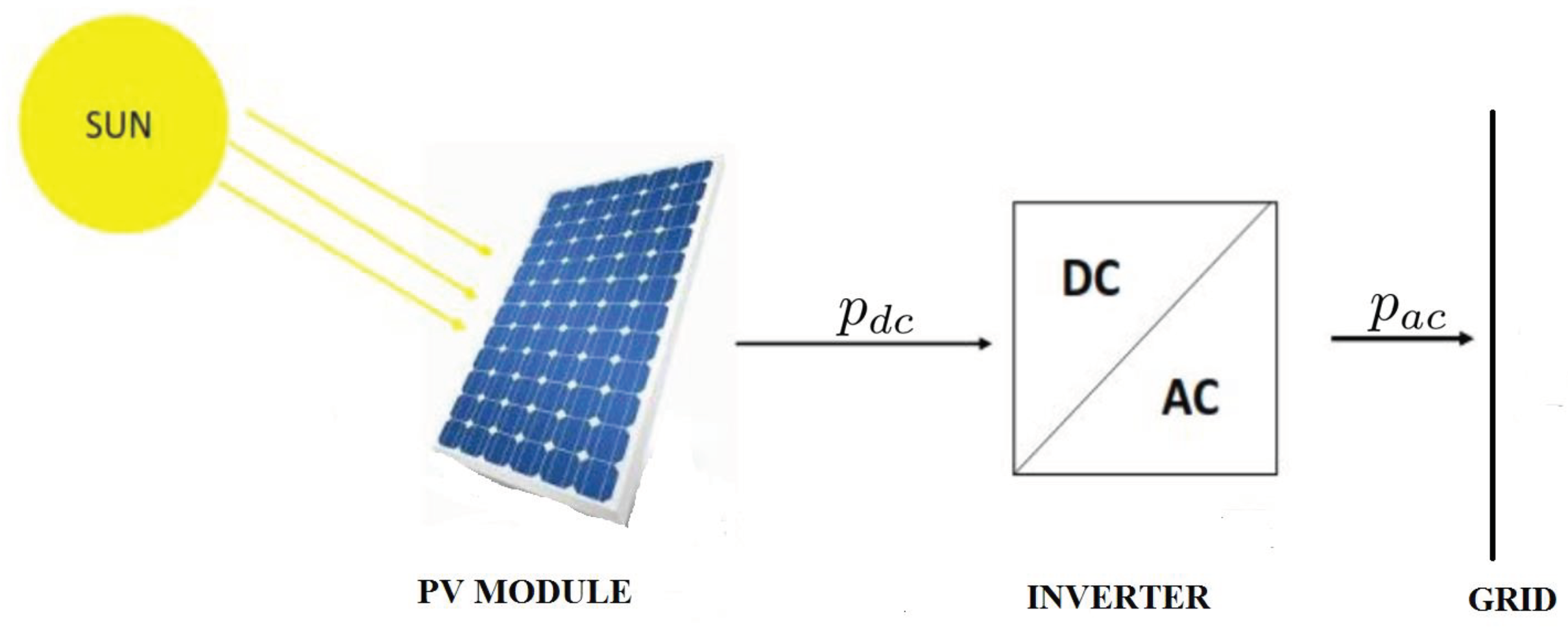
A user on node is generically allowed to have a PV generation unit. The output of the optimization problem to be described will yield the optimal decisions with respect to PV installation. For the PV module, the variable of interest is the panel area, which is denoted by for node n and home ℓ. The PV setup is shown in Figure 2. The nameplate DC rating of the PV module at node and home , denoted by , is given by
where is the module efficiency and is the solar irradiance at standard test conditions (STC) and is equal to [10].
For a PV-enabled user, the DC power output of the PV module is governed by solar irradiance conditions. Assume that, for user at node , the uncertainty in solar irradiance and loads can be characterized by the finite set of T scenarios indexed by the set . Denote by the plane-of-array irradiance (in ) at node n and scenario t. The DC power output of the PV module denoted by is given by [11]
2.2. Inverter Model
At node and user , let denote the nameplate apparent power capability of the inverter. Furthermore, denote respectively by and the AC real and reactive power output injected to the grid per scenario . Assuming that the inverter efficiency is a constant given by , the real AC power injected into the grid equals
where d is the derating factor. Equation (3) shows that, in cases of excess available AC power generation due to exceedingly high irradiances, the output of the inverter is clipped to match its apparent power capability . This clipping effect is accounted for in the PV Watts calculator [11]. By substituting the right-hand side of Equation (2) into Equation (3), the operational constraints on and , expressed in terms of sizing variables and , are given as follows:
Constraint (4b) is a second-order cone (SOC) while constraint (4a) is nonconvex as the right-hand side is the minimum of two expressions that depend respectively on variables and . In Section 2.2.1 and Section 2.2.2, we detail two engineering designs that easily bypass this non-convexity. The designs are based on assumptions on the DC:AC ratio which for and is denoted by and is defined as
The first design, referred to as the optimal design, is explained in Section 2.2.1 and is based on the requirement that the DC:AC ratio of all PVs to be installed must be smaller than a maximum pre-specified DC:AC ratio denoted by . Concretely, for all and , the following is required:
The second design, referred to as the alternative design, is explained in Section 2.2.2 and considers that the DC:AC ratio is known for all modules.
2.2.1. Optimal Inverter Sizing
We first present an assumption on solar irradiances and the maximum pre-specified DC:AC size.
Assumption 1.
The historical data on solar irradiance is such that the following holds:
where .
We have verified, based on the solar irradiance data obtained from PVWatts for San Antonio, that, for the common DC:AC ratio size of , the condition in Assumption 1 (Equation (7)), is satisfied. Based on Assumption 1, the following proposition offers a path to bypass the nonconvexity in (4a).
Proposition 1.
By Assumption 1, Constraint (4a) reduces to the ensuing linear constraint:
Proof.
Due to Equation (7), it holds that
Substituting for in (9b) using (1) yields
Equation (10) suggests that the minimum in (4a) always takes on its first argument, which implies (8). □
Notice that if Assumption 1 is not satisfied, then due to (4b), the placement and sizing optimization problem using (10) in place of (4a) implicitly enforces a maximum allowable DC:AC ratio, denoted by , satisfying
2.2.2. Alternative Inverter Sizing
In case of a pre-specified value of , the next proposition provides a convex reformulation of (4a).
Proposition 2.
Under specified DC:AC ratio , (4a) reduces to the following two linear constraints:
Proof.
Constraint (12b) simply states that the DC:AC ratio is fixed at . By substituting (12b) in place of in (4a), we arrive at (12a). □
Notice that, in (12a), the terms inside the minimum are dependent on fixed parameters and known scenarios and not on decision variables.
2.3. Placement and Sizing Constraints
A binary variable is introduced for the PV placement as follows:
where signifies the presence of a unit at node n and home ℓ. The number of installations per node is limited by a budget as follows:
The following constraint is required for the set of nodes where PV installation is not allowed:
There is a minimum nameplate apparent power capacity available for installation denoted by . Furthermore, the nameplate apparent power capacity should be limited within a factor of the AC production. Therefore, the following constraint is enforced:
In reference (16), the expression is the unclipped nominal AC real power generation from the PV module at STC and refers to a constant that shows how larger the nameplate apparent power capacity can be in comparison to the unclipped real power generation at STC.
Finally, there is a minimum and maximum of solar panel size available for installation respectively denoted by and yielding
2.4. Real Power and Reactive Power Consumption
Each user node consumes real and reactive power. These values are dependent on user behavior and are thus random variables. It can be assumed that these random variables are incorporated and accounted for in the set of scenarios . In particular, at a user node , user , per scenario , real power consumption and reactive power consumption are given by and , respectively.
2.5. Power Flows
As the real and reactive power generation or consumption changes from user to user at each scenario, the power flows in the distribution network will also be scenario dependent. Let and respectively be the real and reactive power flow going into node n at scenario t; and be the squared magnitude of the voltage phasor at node n at scenario t. The LinDistFlow approximation of the power flow equations is adopted here [36] (where all quantities are measured per unit):
In reference (18), is the reactive power injected by shunt capacitor at node n at nominal voltage, and and are respectively the resistance and reactance of line n. The voltage at the substation is considered to be fixed at one per unit. For every user node , the voltage should be maintained close to the substation voltage. Thus, the following constraint carries out the voltage regulation:
where is a small value, usually 0.03 or 0.05.
2.6. Objective Function
Three objectives are considered:
- PV panel area cost for and . The cost per is represented by .
- Inverter nameplate apparent power capacity cost denoted by for and . The cost per is represented by .
- The term that captures thermal losses [4] multiplied by the price, denoted by , that utility buys from the market.
2.7. Optimization Problem
Let us introduce the following collection of variables:
Then, according to Section 2.6, the objective function is written as
2.7.1. Placement and Sizing with Optimal Inverter Design
Under Assumption 1, the overall optimization problem is as follows:
The solution of (22) yields the power flows and voltages at every node and scenario , as well as the real and reactive power injected into the grid at every node , user , and scenario . Furthermore, the binary installation variables determine the optimal placement of the PV units while variables and respectively determine the PV nameplate apparent power capability and panel area. Problem (22) is a MISOCP due to the binary variables and the SOC (4b).
2.7.2. Placement and Sizing with Alternative Inverter Design
With a specified DC:AC ratio, the optimal placement and sizing problem is given by
which is similar to (22) except for the fact that the two linear constraints of (12) replace (10).
The next section details the input parameters required for the optimization problems (22) and (22′), and gives the overall design procedure.
3. Numerical Data for Experiments and Design Procedure
This section details the distribution feeder used to test the method (Section 3.1), the generation of load (Section 3.2) and irradiance scenarios (Section 3.3), and the sources for installation and electricity costs (Section 3.4). Section 3.5 outlines the overall design procedure.
3.1. The Test Network
The IEEE 34-node distribution test feeder [37], shown in Figure 3, has been selected for the numerical studies. Node 1 is the substation and the remaining nodes constitute . The values for line impedances are provided in Table 1 while the values of peak real and reactive loads as well as shunt capacitors are included in Table 2. Voltage and power bases for the network are respectively and .
The set of nodes where PV installation is not allowed is given by . Parameters required for the optimization problem (22) are given in Table 3. Specifically regarding the maximum panel area , we have surveyed 348,000 detached single-family homes in San Antonio and have selected the minimum home size as the maximum available panel area [38].
3.2. Load Scenarios and Allocation of Users per Node
The load is assumed to operate in three scenarios: (1) at peak consumption, (2) at 150 % of peak consumption, and (3) at 50 % of peak consumption. These three scenarios are combined with irradiance scenarios elaborated in Section 3.3.
The allocation of users to nodes is as follows. Based on [39], the average residential load consumption is . If the load of a particular node is less than or equal to , then that node is considered to have one user. If the load of a particular node is greater than , then the number of users of that node is found by dividing the load by . The resulting number of users per node is shown in Table 4.
3.3. Irradiance Scenarios
Irradiance scenarios are based on the NREL PVWatts calculator. PVWatts includes solar resource data, system info, and the DC and AC output generation. First, the zip code 78249 is selected for the location. PVWatts obtains weather data including solar irradiance for the selected location. The default input parameters are then input to the PVWatts calculator. The output of the PVWatts calculator gives two sets of irradiance data. One is monthly energy (solar radiation), i.e., the average monthly plane-of-array (POA) irradiance , and the other is the hourly POA irradiance . These are related by the following Equation [11]:
Irradiance scenarios are then calculated by dividing with the average number of non-zero irradiance hours in month m and are shown in Table 5. The total number of scenarios is thus , i.e., 3 load scenarios × 12 irradiance scenarios. For and , is the peak load (see Table 2); for , is of the peak load, and for , is of the peak load. Table 5 shows the irradiance scenarios for scenarios . The same values are repeated for all three load cases.
3.4. Installation and Electricity Costs
The cost function parameters are given next:
- Electricity Costs: According to the Wholesale Electricity Market Data of 2016 [41], a representative price of electricity at which the utility buys from the market is .
3.5. Design Procedure
An overview of our proposed approach is presented in the diagram of Figure 4. In this diagram, the first block collects the required input parameters required by the optimization problems (22) and (22′). This block also provides the appropriate table or section in the paper that details the specific parameter values used in this study.
The optimization problems are then programmed in the CVX toolbox [42,43]—a specialized modeling package designed for specifying and solving convex programs. In particular, the CVX toolbox provides an automated way to translate the mathematical form of convex problems (22) and (22′) to their standard optimization form. The standard form is understood by an optimization solver, which is called from inside CVX. The outputs obtained by CVX are the optimal placement and sizing decisions as well as estimates of nodal voltage levels and branch power flows during various operation scenarios, as depicted in the third block.
This study is tested using the previously mentioned available data, but the optimization model is very general, and can accept any combination of feeder, load and irradiance scenarios, and costs as inputs. The numerical results obtained by the procedure of Figure 4 are presented and analyzed in the next section.
4. Results and Discussion
In this section, we examine the results of the placement and sizing problem in terms of costs, voltage regulation, number of PV installations, as well as panel area sizes. The first part, Section 4.1, discusses the results solved by problem (22). The second part, Section 4.2, provides a comparison between the solutions of problem (22) and (22′).
4.1. Results of Placement and Sizing with Optimal Inverter Design
Voltage regulation is the task of maintaining voltages across the distribution network close to the nominal value of the substation voltage. When there are no PV units present, the feeder voltage profile obtained by running the load-flow using the LinDistFlow is depicted in Figure 5. It can be observed that, when consumption is at of the peak load, voltages drop as nodes get farther away from the substation. When a maximum installation of one PV unit per node is allowed, the optimal solution from problem (22) yields the voltage profile in Figure 6 where every nodal voltage in the system remains within appropriate bounds for every generation scenario. This constraint is enforced via (19), where . This simple experiment motivates the voltage regulation benefits of placing PV generation units in distribution networks. In what follows, we will examine the optimal setups in cases where more homes per node are allowed to install PV units.
The number of installations allowed per node for is shown in Figure 7. By observing Figure 7, it is clear that most of the installations are allowed at nodes 11, 19, and 20 which are the terminal nodes of the radial network; compare with Figure 3. The voltage drop at those particular nodes are high, and more installations are required.
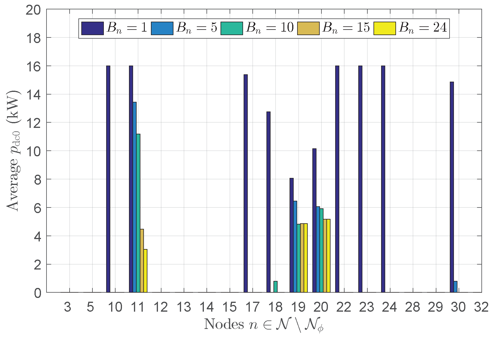
Figure 8 depicts the average value of the panel area of all the installations allowed per node for . For example, if , the optimal locations of installations are nodes 11, 19, and 20. Out of the seven homes of node 20, only five homes have installations with an average panel area of 38.7878 and this value is shown in Figure 8 for node 20 and . The same applies for . The average nameplate DC rating of the PV module is depicted in Figure 9, which is calculated using through (1).
Figure 10 depicts the average value of the inverter capacity of all the installations allowed per node for . For example, when , the installations occur on nodes 11, 19, and 20. Out of the seven homes of node 20, five homes have installations with average inverter capacity of and this value is displayed for node 20 and . The same applies for .
Using Figure 8 and Figure 10, the maximum of the average panel area and the maximum of the average inverter capacity for each are listed in Table 6. For example, it follows from Figure 8 that, if , the installations are allowed at nodes 11, 19, and 20. The average values of the panel area for allowed installations at nodes 11, 19, and 20 are 83.95 , 40.33 , and 37.92 , respectively. The maximum of the three values is 83.9548 , which corresponds to the maximum of the average panel area for . The same is applicable for . The maximum of the average inverter capacity is given as the maximum value of the average inverter capacity for each of the bar plots in Figure 10. For example, it is inferred from Figure 10 that, when , the installations are allowed at nodes 11, 19, and 20. The average values of the inverter capacity for allowed installations at nodes 11, 19, and 20 are, respectively, , , and . The maximum of the aforementioned three values is , which corresponds to the maximum of the average inverter capacity for . Table 6 shows that, as the number of installations allowed per node increases, the maxima of the average panel area and the average inverter capacity decrease.
Table 7 lists the optimal value, installation cost, including inverter and DC cost, and thermal loss cost. From Table 7, it is observed that the optimal value and the installation cost remain the same for . It is also observed that the DC costs remain the same for and although there is a significant difference between the maximum of the average panel area for and in Table 6. The reason is that the sum of the panel areas of all the allowed installations per node for and is the same and is equal to . A similar observation holds for and . In this work, the maximum value of is relatively large, that is, (cf. Section 3.1). Therefore, the results for give large panel sizes, but, for larger values of , e.g., for , the resulting panel area sizes are realistic.
4.2. Comparison between Optimal and Alternative Inverter Design
Figure 11 and Figure 12 provide the comparison of panel areas and inverter capacities obtained from the optimal inverter design of (22) and the alternative inverter design of (22′) with . The panel areas coming from the alternative design are nearly three times higher in comparison to the panel areas offered from the optimal design. The main finding is that the same inverter capacity can be achieved by both designs; however, the panel area resulting from the optimal design of (22) is much smaller than those of (22′). Optimal inverter sizing is dictated by the feeder reactive power support needs, which are determined by the load and irradiance scenarios through the power flow equations of (22).
Table 8 depicts the comparison between the maximum of average panel areas and the maximum of average inverter capacities resulting from the optimal design of (22) and the alternative design (22′) with . It is observed that although the maximum of average panel areas from (22′) is three times higher than the maximum of average panel area from (22), the maximum of average inverter capacities is almost the same for both designs. It is concluded that the model given by (22) is less costly compared to the alternative model of (22′) since the same inverter capacity is achieved by smaller panel areas. To bear witness, Table 9 shows the optimal values, installation costs, and thermal loss costs for the two designs with . Table 9 reveals that the total cost and the installation costs of (22) are smaller than those of (22′).
5. Conclusions
This paper develops a two-stage stochastic program that serves as a tool for optimally determining the placing and sizing of PV units in distribution grids. In particular, a novel analytical PV model that justifiably captures the mapping from solar irradiance to power injection is introduced in this work and is incorporated into the system-level study. By modeling the stochasticity of solar irradiance and loads via a finite set of scenarios and incorporating them in the power flow equations, optimal PV locations and sizes that minimize thermal loss costs are determined via two-stage stochastic programming. A comparison between two designs, one with pre-specified DC:AC ratio and another with pre-specified maximum DC:AC ratio based on historical data, shows that the latter method reduces costs by reducing the panel area. Overall, this paper develops a rigorous framework that can guide electric utility companies in identifying optimal locations for PV placement and sizing, assist with targeting customers with appropriate incentives, and encourage solar adoption.
Author Contributions
Conceptualization, N.G. and J.G.; Methodology, N.G. and M.B.; Software, L.Y.; Validation, M.B. and J.G.; Formal Analysis, N.G. and M.B.; Investigation, L.Y.; Writing—Original Draft Preparation, M.B. and L.Y.; Writing—Review and Editing, M.B. and N.G.; Visualization, L.Y.; Supervision, N.G.; Funding Acquisition, N.G. and J.G.
Funding
This work was supported by the National Science Foundation Grants CCF-1421583 and ECCS-1462404. This project and the preparation of this study were also funded in part by monies provided by CPS Energy (San Antonio, TX, USA) through an agreement with the University of Texas at San Antonio.
Conflicts of Interest
The authors declare no conflict of interest. The funders had no role in the design of the study; in the collection, analyses, or interpretation of data; in the writing of the manuscript, or in the decision to publish the results.
References
- Pitt, D.; Michaud, G. Analyzing the Costs and Benefits of Distributed Solar Generation in Virginia. Available online: http://mdvseia.org/wp-content/uploads/2014/12/SSG-Value-of-Solar-Study-Final-10-31-14.pdf (accessed on 9 January 2019).
- U.S. Department of Energy. Systems Integration. Available online: https://energy.gov/eere/sunshot/systems-integration (accessed on 9 January 2019).
- CPS Energy. Solar Power. Available online: https://www.cpsenergy.com/en/about-us/programs-services/energy-generation/solar-power.html (accessed on 9 January 2019).
- Xcel Energy Services Inc. Costs and Benefits of Distributed Solar Generation on the Public Service Company of Colorado System Study. Available online: http://www.eei.org/issuesandpolicy/generation/ NetMetering/Documents/Costs%20and%20Benefits%20of%20Distributed%20Solar%20Generation% 20on%20the%20Public%20Service%20Company%20of%20Colorado%20System%20Xcel%20Energy. pdf (accessed on 9 January 2019).
- Kanwar, N.; Gupta, N.; Niazi, K.; Swarnkar, A.; Bansal, R. Simultaneous allocation of distributed energy resource using improved particle swarm optimization. Appl. Energy 2017, 185, 1684–1693. [Google Scholar] [CrossRef]
- Armendáriz, M.; Heleno, M.; Cardoso, G.; Mashayekh, S.; Stadler, M.; Nordström, L. Coordinated microgrid investment and planning process considering the system operator. Appl. Energy 2017, 200, 132–140. [Google Scholar] [CrossRef] [Green Version]
- Silvestre, M.D.; Cascia, D.L.; Sanseverino, E.R.; Zizzo, G. Improving the energy efficiency of an islanded distribution network using classical and innovative computation methods. Util. Policy 2016, 40, 58–66. [Google Scholar] [CrossRef]
- Valdberg, A.J.; Dwyer, M.W. Distribution Resources Plan Rulemaking (R. 14-08-013) Locational Net Benefit Analysis Working Group Final Report. Available online: http://drpwg.org/wp-content/uploads/2016/07/R1408013-et-al-SCE-LNBA-Working-Group-Final-Report.pdf (accessed on 9 January 2019).
- Tonkoski, R.; Turcotte, D.; El-Fouly, T.H.M. Impact of high PV penetration on voltage profiles in residential neighborhoods. IEEE Trans. Sustain. Energy 2012, 3, 518–527. [Google Scholar] [CrossRef]
- National Renewable Energy Laboratory. PVWatts Documentation. Available online: http://pvwatts.nrel.gov (accessed on 9 January 2019).
- Dobos, A.P. PVWatts Version 5 Manual. Technical Report NREL/TP-6A20-62641; National Renewable Energy Laboratory, 2014. Available online: http://www.nrel.gov/docs/fy14osti/62641.pdf (accessed on 9 January 2019).[Green Version]
- Georgilakis, P.S.; Hatziargyriou, N.D. Optimal Distributed Generation Placement in Power Distribution Networks: Models, Methods, and Future Research. IEEE Trans. Power Syst. 2013, 28, 3420–3428. [Google Scholar] [CrossRef]
- Keane, A.; Ochoa, L.F.; Borges, C.L.T.; Ault, G.W.; Alarcon-Rodriguez, A.D.; Currie, R.A.F.; Pilo, F.; Dent, C.; Harrison, G.P. State-of-the-Art Techniques and Challenges Ahead for Distributed Generation Planning and Optimization. IEEE Trans. Power Syst. 2013, 28, 1493–1502. [Google Scholar] [CrossRef] [Green Version]
- Kazmi, S.A.A.; Shahzad, M.K.; Shin, D.R. Multi-Objective Planning Techniques in Distribution Networks: A Composite Review. Energies 2017, 10, 208. [Google Scholar] [CrossRef]
- Ehsan, A.; Yang, Q. Optimal integration and planning of renewable distributed generation in the power distribution networks: A review of analytical techniques. Appl. Energy 2018, 210, 44–59. [Google Scholar] [CrossRef]
- Naik, S.N.G.; Khatod, D.K.; Sharma, M.P. Analytical approach for optimal siting and sizing of distributed generation in radial distribution networks. IET Gener. Transm. Distrib. 2015, 9, 209–220. [Google Scholar] [CrossRef]
- Al-Sabounchi, A.; Gow, J.; Al-Akaidi, M. Simple procedure for optimal sizing and location of a single photovoltaic generator on radial distribution feeder. IET Renew. Power Gener. 2014, 8, 160–170. [Google Scholar] [CrossRef]
- Vita, V. Development of a Decision-Making Algorithm for the Optimum Size and Placement of Distributed Generation Units in Distribution Networks. Energies 2017, 10, 1433. [Google Scholar] [CrossRef]
- Yammani, C.; Maheswarapu, S.; Matam, S.K. A Multi-objective Shuffled Bat algorithm for optimal placement and sizing of multi distributed generations with different load models. Int. J. Electr. Power Energy Syst. 2016, 79, 120–131. [Google Scholar] [CrossRef]
- Fu, X.; Chen, H.; Cai, R.; Yang, P. Optimal allocation and adaptive VAR control of PV-DG in distribution networks. Appl. Energy 2015, 137, 173–182. [Google Scholar] [CrossRef]
- Li, Y.; Feng, B.; Li, G.; Qi, J.; Zhao, D.; Mu, Y. Optimal distributed generation planning in active distribution networks considering integration of energy storage. Appl. Energy 2018, 210, 1073–1081. [Google Scholar] [CrossRef]
- Sheng, W.; Liu, K.Y.; Liu, Y.; Meng, X.; Li, Y. Optimal Placement and Sizing of Distributed Generation via an Improved Nondominated Sorting Genetic Algorithm II. IEEE Trans. Power Del. 2015, 30, 569–578. [Google Scholar] [CrossRef]
- Bhullar, S.; Ghosh, S. Optimal Integration of Multi Distributed Generation Sources in Radial Distribution Networks Using a Hybrid Algorithm. Energies 2018, 11, 628. [Google Scholar] [CrossRef]
- Kumar, M.; Nallagownden, P.; Elamvazuthi, I. Optimal Placement and Sizing of Renewable Distributed Generations and Capacitor Banks into Radial Distribution Systems. Energies 2017, 10, 811. [Google Scholar] [CrossRef]
- Zhang, S.; Cheng, H.; Li, K.; Tai, N.; Wang, D.; Li, F. Multi-objective distributed generation planning in distribution network considering correlations among uncertainties. Appl. Energy 2018, 226, 743–755. [Google Scholar] [CrossRef]
- Foster, J.D.; Berry, A.M.; Boland, N.; Waterer, H. Comparison of Mixed-Integer Programming and Genetic Algorithm Methods for Distributed Generation Planning. IEEE Trans. Power Syst. 2014, 29, 833–843. [Google Scholar] [CrossRef]
- Wang, Z.; Chen, B.; Wang, J.; Kim, J.; Begovic, M.M. Robust Optimization Based Optimal DG Placement in Microgrids. IEEE Trans. Smart Grid 2014, 5, 2173–2182. [Google Scholar] [CrossRef]
- Wang, Z.; Chen, B.; Wang, J.; Begovic, M.M. Stochastic DG Placement for Conservation Voltage Reduction Based on Multiple Replications Procedure. IEEE Trans. Power Del. 2015, 30, 1039–1047. [Google Scholar] [CrossRef]
- Luo, L.; Gu, W.; Zhang, X.P.; Cao, G.; Wang, W.; Zhu, G.; You, D.; Wu, Z. Optimal siting and sizing of distributed generation in distribution systems with PV solar farm utilized as STATCOM (PV-STATCOM). Appl. Energy 2018, 210, 1092–1100. [Google Scholar] [CrossRef]
- Santos, S.F.; Fitiwi, D.Z.; Shafie-Khah, M.; Bizuayehu, A.W.; Cabrita, C.M.P.; Catalão, J.P.S. New Multistage and Stochastic Mathematical Model for Maximizing RES Hosting Capacity—Part I: Problem Formulation. IEEE Trans. Sustain. Energy 2017, 8, 304–319. [Google Scholar] [CrossRef]
- Dall’Anese, E.; Giannakis, G.B. Optimal Distributed Generation Placement in Distribution Systems via Semidefinite Relaxation. In Proceedings of the 2013 Asilomar Conference on Signals, Systems and Computers, Pacific Grove, CA, USA, 3–6 November 2013; pp. 369–373. [Google Scholar] [CrossRef]
- Bazrafshan, M.; Gatsis, N.; Dall’Anese, E. Placement and Sizing of Inverter-Based Renewable Systems in Multi-Phase Distribution Networks. IEEE Trans. Power Systems 2018, in press. [Google Scholar] [CrossRef]
- Conejo, A.J.; Carrión, M.; Morales, J.M. Decision Making under Uncertainty in Electricity Markets; Springer: New York, NY, USA, 2010. [Google Scholar]
- Bazrafshan, M.; Gatsis, N. Risk-averse placement and sizing of photovoltaic inverters in radial distribution networks. In Proceedings of the 2015 49th Asilomar Conference on Signals, Systems and Computers, Pacific Grove, CA, USA, 8–11 November 2015; pp. 885–889. [Google Scholar] [CrossRef]
- Bazrafshan, M.; Gatsis, N. Placing and sizing distributed photovoltaic generators for optimal reactive power compensation. In Proceedings of the 2015 IEEE Global Conference on Signal and Information Processing (GlobalSIP), Orlando, FL, USA, 14–16 December 2015; pp. 1136–1140. [Google Scholar] [CrossRef]
- Turitsyn, K.; Šulc, P.; Backhaus, S.; Chertkov, M. Options for control of reactive power by distributed photovoltaic generators. Proc. IEEE 2011, 99, 1063–1073. [Google Scholar] [CrossRef]
- IEEE Distribution Planning Working Group. Radial distribution test feeders. IEEE Trans. Power Syst. 1991, 6, 975–985. [Google Scholar] [CrossRef]
- Gomez, J.D.; Elnakat, A.; Wright, M.; Keener, J. Analysis of the energy index as a benchmarking indicator of potential energy savings in the San Antonio, Texas single-family residential sector. Energy Efficien. 2014, 8, 577–593. [Google Scholar] [CrossRef]
- Willis, H.L. Power Distribution Planning Reference Book; CRC Press: Boca Raton, FL, USA, 2004. [Google Scholar]
- Cameron, C.P.; Goodrichg, A.C. The levelized cost of energy for distributed PV: A parametric study. In Proceedings of the 2010 35th IEEE Photovoltaic Specialists Conference, Honolulu, HI, USA, 20–25 June 2010; pp. 529–534. [Google Scholar] [CrossRef]
- Energy Information Administration. Wholesale Electricity and Natural Gas Market Data. Available online: http://www.eia.gov/electricity/wholesale (accessed on 7 February 2017).
- CVX Research, Inc. CVX: Matlab Software for Disciplined Convex Programming, version 2.0. Available online: http://cvxr.com/cvx/ (accessed on 25 November 2017).
- Grant, M.; Boyd, S. Graph implementations for nonsmooth convex programs. In Recent Advances in Learning and Control; Blondel, V., Boyd, S., Kimura, H., Eds.; Lecture Notes in Control and Information Sciences; Springer-Verlag Limited: Cham, Switzerland, 2008; pp. 95–110. [Google Scholar]
Figure 1.
A radial distribution network with users at each node.

Figure 2.
The setup of the PV unit and its interface with the distribution grid.

Figure 3.
IEEE 34-node distribution test feeder [37].
Figure 3.
IEEE 34-node distribution test feeder [37].

Figure 4.
A diagram of the approach. The first block collects and organizes the input parameters required for the optimization problem. Refer to the tables in parenthesis for specific values of these paremeters. The second block portrays the optimization problem that are carried out by CVX. Upon solving the optimization problems, optimal placement and sizing decisions as well as estimates of nodal voltages and branch power flows are output to the third block.

Figure 5.
Voltage profile with no PV installations allowed.

Figure 6.
Voltage profile with one PV installation allowed per node ().

Figure 7.
Total number of installations per node.

Figure 8.
Average panel area per node.

Figure 9.
Average nameplate DC rating of the PV module.

Figure 10.
Average inverter capacity.
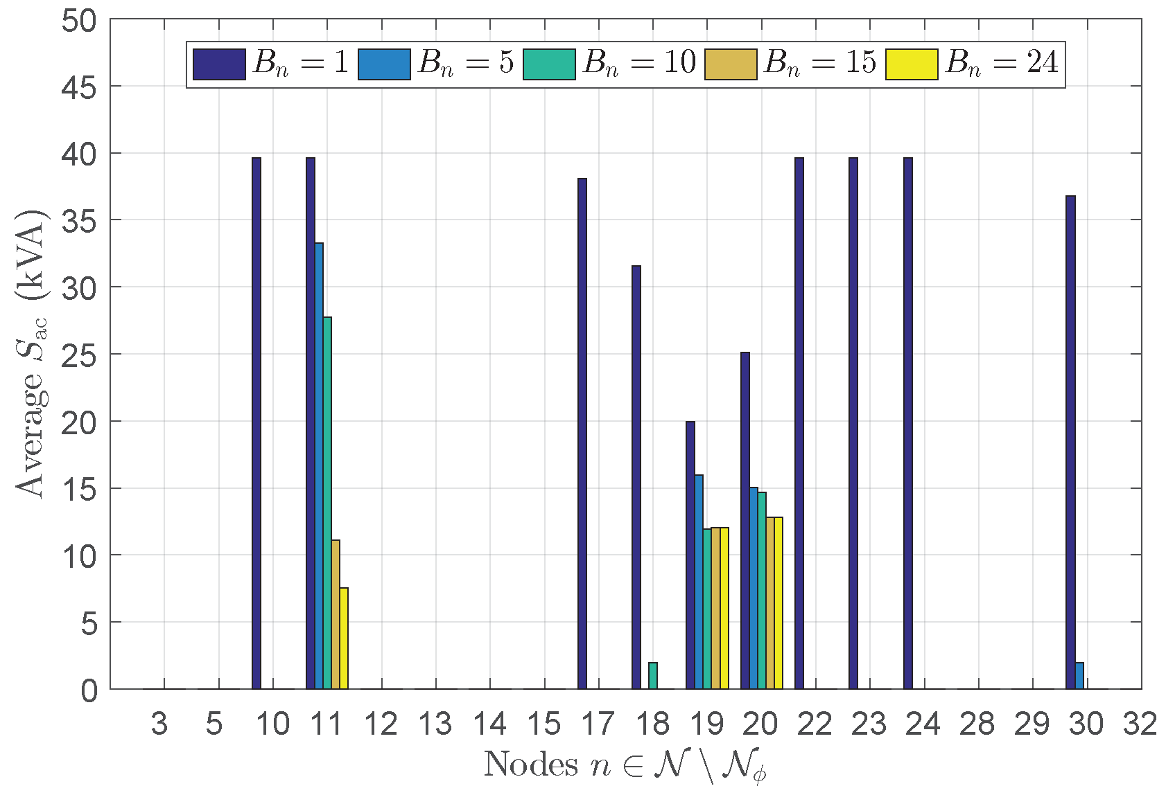
Figure 11.
Comparison of average panel area per node.

Figure 12.
Comparison of average per node.


Table 1.
Line resistance and reactance [35].
Table 1.
Line resistance and reactance [35].
| Line | Line | Line | ||||||
|---|---|---|---|---|---|---|---|---|
| () | () | () | () | () | () | |||
| 1 | 0.0005 | 0.0005 | 12 | 0.0013 | 0.0007 | 23 | 0.0002 | 0.0001 |
| 2 | 0.0004 | 0.0004 | 13 | 0.0002 | 0.0002 | 24 | 0.0000 | 0.0000 |
| 3 | 0.0065 | 0.0066 | 14 | 0.0060 | 0.0044 | 25 | 0.0108 | 0.0080 |
| 4 | 0.0012 | 0.0013 | 15 | 0.0000 | 0.0000 | 26 | 0.0002 | 0.0001 |
| 5 | 0.0076 | 0.0077 | 16 | 0.0017 | 0.0013 | 27 | 0.0068 | 0.0053 |
| 6 | 0.0060 | 0.0061 | 17 | 0.0008 | 0.0006 | 28 | 0.0014 | 0.0011 |
| 7 | 0.0001 | 0.0001 | 18 | 0.0014 | 0.0011 | 29 | 0.0006 | 0.0004 |
| 8 | 0.0007 | 0.0004 | 19 | 0.0003 | 0.0002 | 30 | 0.0001 | 0.0001 |
| 9 | 0.0205 | 0.0109 | 20 | 0.0001 | 0.0001 | 31 | 0.0007 | 0.0004 |
| 10 | 0.0059 | 0.0031 | 21 | 0.0004 | 0.0003 | 32 | 0.0109 | 0.0408 |
| 11 | 0.0030 | 0.0022 | 22 | 0.0011 | 0.0008 | 33 | 0.0021 | 0.0022 |
Table 2.
Peak real and reactive load and shunt capacitors [35].
Table 2.
Peak real and reactive load and shunt capacitors [35].
| Bus | Peak | Peak | Bus | Peak | Peak |
|---|---|---|---|---|---|
| () | () | () | () | ||
| 3 | 0.1100 | 0.0580 | 20 | 0.1340 | 0.0820 |
| 5 | 0.0320 | 0.0160 | 22 | 0.8280 | 0.6400 |
| 10 | 0.0680 | 0.0340 | 23 | 0.0900 | 0.0460 |
| 11 | 0.2700 | 0.1400 | 24 | 0.1660 | 0.1180 |
| 12 | 0.0100 | 0.0040 | 28 | 0.0080 | 0.0040 |
| 13 | 0.0800 | 0.0400 | 29 | 0.0300 | 0.0140 |
| 14 | 0.0080 | 0.0040 | 30 | 0.4120 | 0.2420 |
| 15 | 0.1040 | 0.0460 | 32 | 0.0040 | 0.0020 |
| 17 | 0.0640 | 0.0340 | Shunt Capacitors () | ||
| 18 | 0.1640 | 0.0860 | 22 | 0.6 | |
| 19 | 0.0560 | 0.0280 | 24 | 0.9 | |
Table 3.
Optimization problem parameters.
| Parameter | Value | Parameter | Value |
|---|---|---|---|
| 11,540 | |||
| C | |||
| d | |||
| 3 | see Section 4 |
Table 4.
No. of users per node .
| Bus | Bus | Bus | Bus | Bus | |||||
|---|---|---|---|---|---|---|---|---|---|
| 3 | 9 | 19 | 5 | 13 | 7 | 28 | 1 | 12 | 1 |
| 5 | 3 | 20 | 7 | 14 | 1 | 29 | 3 | 24 | 4 |
| 10 | 5 | 22 | 1 | 15 | 1 | 30 | 24 | 18 | 14 |
| 11 | 22 | 23 | 8 | 17 | 5 | 32 | 1 |
Table 5.
Irradiance scenario generation.
| Month | Average POA | Average no. | Scenario |
|---|---|---|---|
| Irradiance | of Hours with | ||
| Non-Zero Irradiance | |||
| January | 3.91 | 11.19 | 0.349 |
| February | 4.68 | 12 | 0.39 |
| March | 5.32 | 12.77 | 0.41 |
| April | 5.55 | 13.2 | 0.420 |
| May | 5.87 | 14.838 | 0.395 |
| June | 6.29 | 15 | 0.42 |
| July | 6.83 | 14.70 | 0.46 |
| August | 6.57 | 13.77 | 0.477 |
| September | 5.87 | 13 | 0.45 |
| October | 5.40 | 12.45 | 0.43 |
| November | 4.47 | 11.33 | 0.39 |
| December | 3.78 | 11 | 0.34 |
Table 6.
Maximum average panel area and average inverter capacity.
| # of Installations | Max. of Average | Max. of Average |
|---|---|---|
| Allowed per node | Panel Area | Inverter Capacity |
| 100.00 | 39.65 | |
| 83.95 | 33.25 | |
| 69.95 | 27.70 | |
| 32.32 | 12.80 | |
| 32.32 | 12.80 |
Table 7.
Optimal values and costs.
| Optimal | Inverter | DC | Thermal | |
|---|---|---|---|---|
| Value | Cost | Cost | Loss Cost | |
| 1,891,670 | 262,230 | 1,629,400 | 57.4959 | |
| 1,576,210 | 218,530 | 1,357,600 | 60.6561 | |
| 1,576,140 | 218,510 | 1,357,600 | 60.6873 | |
| 1,576,090 | 218,520 | 1,357,500 | 60.6467 | |
| 1,576,090 | 218,520 | 1,357,500 | 60.6478 |
Table 8.
Comparison of optimal and alternative design—maximum average panel area and average inverter capacity ().
Table 8.
Comparison of optimal and alternative design—maximum average panel area and average inverter capacity ().
| Method | Max. of Average | Max. of Average |
|---|---|---|
| Panel Area | Inverter Capacity | |
| Optimal | 32.32 | 12.8 |
| Alternative | 93.6115 | 13.6 |
Table 9.
Comparison of optimal and alternative design—Optimal values and costs ().
| Method | Optimal | Inverter | DC | Thermal Loss |
|---|---|---|---|---|
| Value | Cost | Cost | Cost | |
| Optimal | 1,576,090 | 219,000 | 136,000 | 60.6702 |
| Alternative | 3,361,030 | 187,500 | 3,173,500 | 61.7727 |
© 2019 by the authors. Licensee MDPI, Basel, Switzerland. This article is an open access article distributed under the terms and conditions of the Creative Commons Attribution (CC BY) license (http://creativecommons.org/licenses/by/4.0/).
Share and Cite
MDPI and ACS Style
Bazrafshan, M.; Yalamanchili, L.; Gatsis, N.; Gomez, J. Stochastic Planning of Distributed PV Generation. Energies 2019, 12, 459. https://doi.org/10.3390/en12030459
AMA Style
Bazrafshan M, Yalamanchili L, Gatsis N, Gomez J. Stochastic Planning of Distributed PV Generation. Energies. 2019; 12(3):459. https://doi.org/10.3390/en12030459
Chicago/Turabian StyleBazrafshan, Mohammadhafez, Likhitha Yalamanchili, Nikolaos Gatsis, and Juan Gomez. 2019. "Stochastic Planning of Distributed PV Generation" Energies 12, no. 3: 459. https://doi.org/10.3390/en12030459
Note that from the first issue of 2016, this journal uses article numbers instead of page numbers. See further details here.