Article

Feasible Islanding Operation of Electric Networks with Large Penetration of Renewable Energy Sources considering Security Constraints

by
Seyed Arash Alavi
1,
Valentin Ilea
2,*,
Alireza Saffarian
1,*,
Cristian Bovo
2,
Alberto Berizzi
2 and
Seyed Ghodratollah Seifossadat
1
1
Electrical Engineering Department, Shahid Chamran University of Ahvaz, Ahvaz 61357-831351, Iran
2
Energy Department, Politecnico di Milano, 20133 Milan, Italy
*
Authors to whom correspondence should be addressed.
Energies 2019, 12(3), 537; https://doi.org/10.3390/en12030537
Submission received: 18 January 2019 / Revised: 2 February 2019 / Accepted: 3 February 2019 / Published: 8 February 2019

Abstract

:
The high penetration of Renewable Energy Sources into electric networks shows new perspectives for the network’s management: among others, exploiting them as resources for network’s security in emergency situations. The paper focuses on the frequency stability of a portion of the grid when it remains islanded following a major fault. It proposes an optimization algorithm that considers the frequency reaction of the relevant components and minimizes the total costs of their shedding. The algorithm predicts the final frequency of the island and the active power profiles of the remaining generators and demands. It is formulated as a Mixed-Integer Non-Linear Programming problem and the high computation time due to a large-size problem is mitigated through a simplified linear version of the model that filters the integer variables. The algorithm is designed to operate on-line and preventively compute the optimal shedding actions to be engaged when islanding occurs. The algorithm is validated for a typical distribution grid: the minimum amount of shedding actions is obtained while the most frequency reactive resources are maintained in operation to assure a feasible frequency. Finally, time-domain simulations show that the optimal solution corresponds to the one at the end of the network’s transients following the islanding.

1. Introduction

In recent years, the Renewable Energy Resources (RES) have dramatically increased their presence at both distribution and sub-transmission levels and thus provided the electric network with a high provision of green energy. However, the RES stochastic nature and the sub-optimal use for network operation led to integration issues, e.g., over-voltages and unpredictable congestions. Nevertheless, the regulatory framework is evolving towards solving these issues and provide an optimal management of the RES. This prioritizes the research of new methodologies for the best ways to exploit the RES. Due to the wide spread of RES in the electric networks, these proposals need to be de-centralized and they generally fall in the field of the so-called smart grids. Recent years have seen a large amount of research being carried out for the normal operation of the electrical networks: papers [1,2,3] and [4,5] are just a few examples for the transmission and distribution levels, respectively. Article [1] shows an optimization procedure to optimally coordinate the DGs at distribution level to fulfill TSO voltage control requirements at the TSO-DSO interface, article [2] proposes a simple, but robust, on-line procedure to mitigate unpredictable congestions, while [3] shows how the RES plants can be exploited to achieve voltage control at sub-transmission level. Moreover, article [4,5] show a series of methodologies to optimally exploit the DGs for voltage control at distribution level. Last, but not least, it is interesting to note that these smart applications require a very good level of the network observability in order to be feasible. The transmission network is highly observable due to a redundancy of measurement devices but there is a major lack at distribution level where interesting research has been developed in order to mitigate this flaw, e.g., [6,7].
The applications previously mentioned are designed for the normal operating conditions of the power system so less attention was given to emergency conditions. Having a large penetration of RESs in the power systems represents an opportunity to exploit them also in emergency conditions, e.g., when the power system has suffered a major fault and a part or parts of it could still be operated in islanding. Thus, this paper focuses on the opportunity to employ the RESs to re-establish the real power balance of a part of the network that has been islanded and are, thus, exploited as providers of frequency restoration services in emergency conditions. Additionally, they are used to warranty the supply permeance of the highest quantity of demand present in the network.
Research in this area has been done in [8,9,10,11,12]. In [8] a method using fast security assessment and coordinated control of Distributed Generation (DGs) is shown. In [9], heuristic methods are engaged to determine the feasible islanding scheme [10]. Moreover, the topic is studied within the microgrids framework in [11,12]. A common characteristic of all these works is that the feasibility of the islanding is either “random” or due to the network’s structure, especially built to withstand deliberate islanding.
An indirect and implicit method to deal with these emergency conditions in power systems is using an appropriate load shedding (LS) scheme proportional to the incident [13,14,15,16,17]. In [13], three different combinational LS have been proposed that use the local frequency and voltage signals. The priority for LS depends on the voltage decay of busses over a period of time. In [14] a new centralized adaptive LS algorithm is proposed which uses the frequency and voltage signals provided by PMUs. The Signal Falling Rate (SFR) model is used to estimate the active power deficit. In [15], two centralized combinational LS are proposed. The first model takes advantage of the SFR model to calculate the power deficit, while an error coefficient is used to compensate the calculation error. The second model uses the incident-based method to estimate the active power deficit. Decentralized LS are proposed in [16] and [17]. Paper [16] uses frequency and voltage information simultaneously, and two criteria, e.g., frequency falling rate (FFR) and voltage falling rate (VFR), are exploited to estimate the active power imbalance and the distance of the bus relay to the center of disturbance respectively. By these additional adaptive logics to the under-frequency (UF) relays, optimal LS have been done. Paper [17] takes the same method of [16], while there is no need to add additional logics to the UF relays. The static thresholds of frequency in regular relays have been substituted by the dynamic frequency threshold calculated according to the bus voltages.
Load shedding schemes that have been suggested for large power systems are no longer appropriate for small areas with high penetrations of RES (e.g., distribution networks). In [18] it is shown that the RESs help the distribution network to be preserved even in island operation. However, a feasible islanding in distribution networks necessitates a proper protecting action like LS or generation cutting. As in normal condition distribution networks are energized by the transmission grid, in most of the cases during islanding there is need to LS. The new challenges for LS due to RES behavior in distribution systems and MGs are analyzed in [19,20,21,22,23,24,25].
An under-frequency load shedding (UFLS) scheme based on directional relays, power flow through feeders, wind and PV measurements is proposed in [19]. Finally, feeders are selected to be disconnected such that the minimum number of DGs are disconnected during the optimal LS. Paper [20] uses under-frequency relay (81L) to do a UFLS action. The optimal shed load at each stage of relay in an islanded MG is calculated by using a Genetic Algorithm (GA). The GA tries to minimize the shed load and maximize the lowest frequency swing. In [21], rate of change of frequency (ROCOF) is estimated and used to set the UF relays. The set points are set dynamically using voltage drops data and they are in coordination with plant protection schemes. So, a decentralized and real time-based LS in presence of high penetration of RESs is proposed in [21]. In [22], a strategy to shed the optimal number of loads after islanding in a distribution network is proposed to prevent the frequency instability. Customers’ willingness to pay (WTP) is considered as a criterion to prioritize the customers for LS action. The WTP is determined when the customers choose the electricity tariff scheme. Paper [23] proposes a multi-stage UFLS for islanded MGs according to estimation of equivalent inertia in presence of high share of RESs. The estimated active power imbalance distributed through loads according to their economic and political influences caused by their interruptions. In [24], control and management strategies of MG DGs, electric vehicles and loads, are proposed to improve the islanding feasibility of MGs by preserving voltage and frequency. The proposed algorithm consists of controllers which set the active power references for MG elements after calculation of active power imbalance. An on-line algorithm in order to improve MG resilience in the moments subsequent to islanding is proposed in [25]. The proposed algorithm manages the MG energy storage systems in coordination with load responsiveness and integration of electric vehicles. The MG energy storage system generates or absorbs active power according to the active power imbalance. This helps to preserve the MG frequency in islanding.
The literature mentioned above deals with protecting actions in distribution systems and MGs in presence of high penetration of RES. Beside [20], all the papers propose simple strategies to set a load shedding logic and/or manage energy storage devices to guarantee a feasible islanding. These strategies rely either on measurements like in [19,21,24,25], or economical merit order in [22,23] or even political criteria in [23]. These strategies do not provide a fine shedding of the demand but a rough one where the group of loads are disconnected. Thus, the imbalance is corrected in a rough way, often resulting in a departure of the frequency value from the nominal one. Paper [20] represents an exception as it uses an actual optimization technique, i.e., a GA. These approaches are generally easy to model and implement and they are able to solve very difficult mathematic models, e.g., discontinuous functions, but they also have practical disadvantages that makes them unreliable for on-line implementation: they are heuristic, not deterministic, hence launched many times with the same input data, different, but very closed to each other, sub-optimal solutions can be found. This can lower the level of trust of a System Operator in the algorithm. Moreover, the GAs do not guarantee a fast computation time. Last, but not the least, these literatures do not consider a proper model for load responsiveness and do not consider the planning of an active power reserve to mitigate future imbalances caused by load variation.
In this paper, an online algorithm is proposed in order to guarantee the feasible islanding of an area of the network with high penetration of RESs, e.g., a distribution network. The algorithm evaluates in real-time and during normal operation of the network the control actions (the demands and/or generators to shed) needed to be activated once the islanding occurs in order to guarantee a continuous and secure operation of surviving island. The algorithm considers the actual frequency-response of the involved components, conventional and renewable generators and the demand, and contains the security constraints necessary to assure the stability of the network after islanding and its long-term reliable operation by calculating an active power reserve to alleviate future imbalances. Due to the nature of the frequency-response characteristics the algorithm is formulated as a Mixed-Integer Non-Linear Programing (MINLP) problem, i.e., an optimization problem characterized by both continuous and discrete variables and containing non-linear equations. The formulated algorithm does not make use of the Power Flow (PF) non-linear equations and so it is not numerically overweight by a large set of non-linear constraints. However, to guarantee a fast computation time a simplified linear model is used to filter the discrete variables of the problem, considerably reducing its size. Thus, the algorithm can find the solution in a few seconds, therefore in a sufficient time to preventively evaluate the network in real-time and efficiently take into account the changes that occur in the network operation. Deterministic techniques are used to solve the problem, so the disadvantages related to the heuristic techniques are alleviated. Furthermore, since the algorithm is an optimization problem the best solution is explicitly found, so rough and simplifying hypothesis are avoided. Finally, the algorithm considers a simple but realistic economic model where the network users’ availability to provide network restoration services is remunerated; thus, the algorithm considers this service as a tradable ancillary service.
Few papers proposing approaches in this particular direction have been published, namely [26,27,28,29]. First, in both papers no economic model is used. The authors of [26] propose a model where the frequency-response characteristics are not present; in order to roughly approximate this, the model uses many user-defined parameters and intuitively formulated constraints. The resulting model is very hard to tune and is case dependent. The authors of [27] propose a model similar to [26] but they focus on the reactive power problem. The authors of [28] consider only the frequency-response of the conventional generators and roughly approximates the frequency-response of RES generators with the one of the conventional generators. Last, but not the least, the authors of [28] solve the proposed MINLP problem using Genetic Algorithms; as explained in the previous paragraph, this approach is not reliable for on-line applications. The authors of [29] propose an algorithm for finding the optimal islands in a network; here, the frequency-response of the synchronous generators is introduced for both the conventional and RES generators. However, the effect of this representation is not clear in the paper as the authors do not discuss it in the results part. The present paper considers explicitly the frequency-response of all the significant networks’ components and proposes a deterministic procedure to tackle the non-linearity of the model and substantially reduce the computation times.
The paper is organized as follows: Section 2 describes the proposed algorithm; Section 3 shows the obtained results when the algorithm is applied for a typical distribution network; while Section 4 discusses the results and the strong points of the algorithm.

2. Island Feasibility Procedure

2.1. Frequency-Response Models of Power System Components

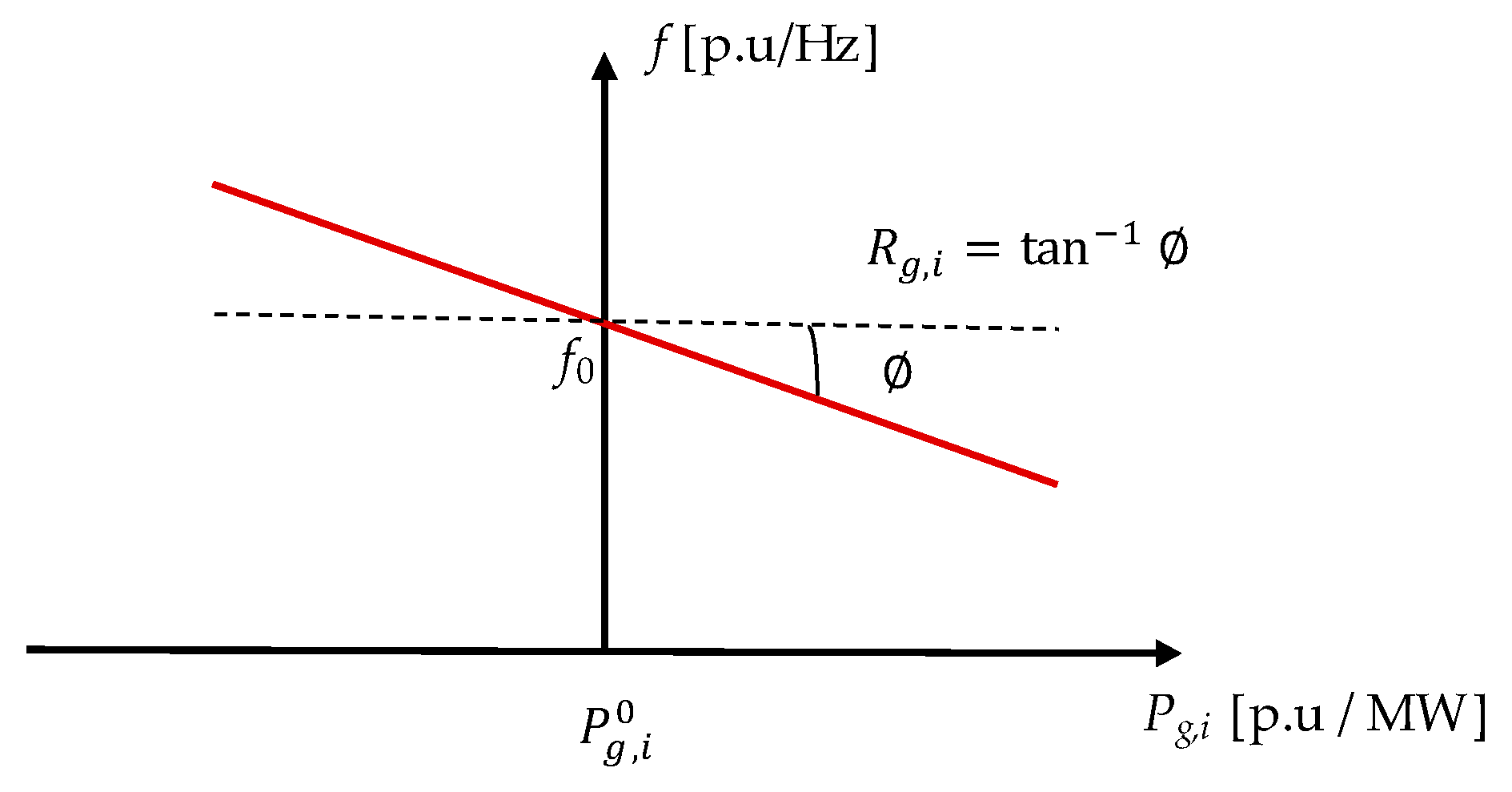
2.1.1. The Synchronous Generator Model

According to [30], it is possible to model the frequency response of a synchronous generator i equipped with governor with a linear P-f characteristic, depicted in Figure 1, where f 0 is the normal operation frequency while P g , i 0 is scheduled active power output of generator i.
Thus, for the ith generator described by the nominal power, P g , i n , slope R g , i of the P-f characteristic and scheduled production of P g , i 0 , the response to an active power imbalance Δ I calculated as the difference between the total demand and the total generation in the network is:
P g , i 1 = P g , i 0 + Δ P g , i
Δ P g , i = Δ I · e g , i e t o t
where, P g , i 1 is the production of the ith generator after the restoration of the power balance in the network; Δ P g , i is the response of the ith generator to Δ I ; e g , i is the regulating energy of the ith generator and e t o t is the total available regulating energy calculated as the sum of e g , i .
Quantity e g , i is calculated as:
e g , i = P g , i n R g , i · f 0
Because of Equation (1), the system frequency becomes,   f 1 :
f 1 = f 0 + Δ f
where Δ f , the frequency variation of the system following the power imbalance restoration, is
Δ f = Δ I e t o t
Thus, according to Equations (1)–(4), the frequency will increase in case of negative imbalance (excess of generation) and will decrease in case of positive imbalance (excess of load).

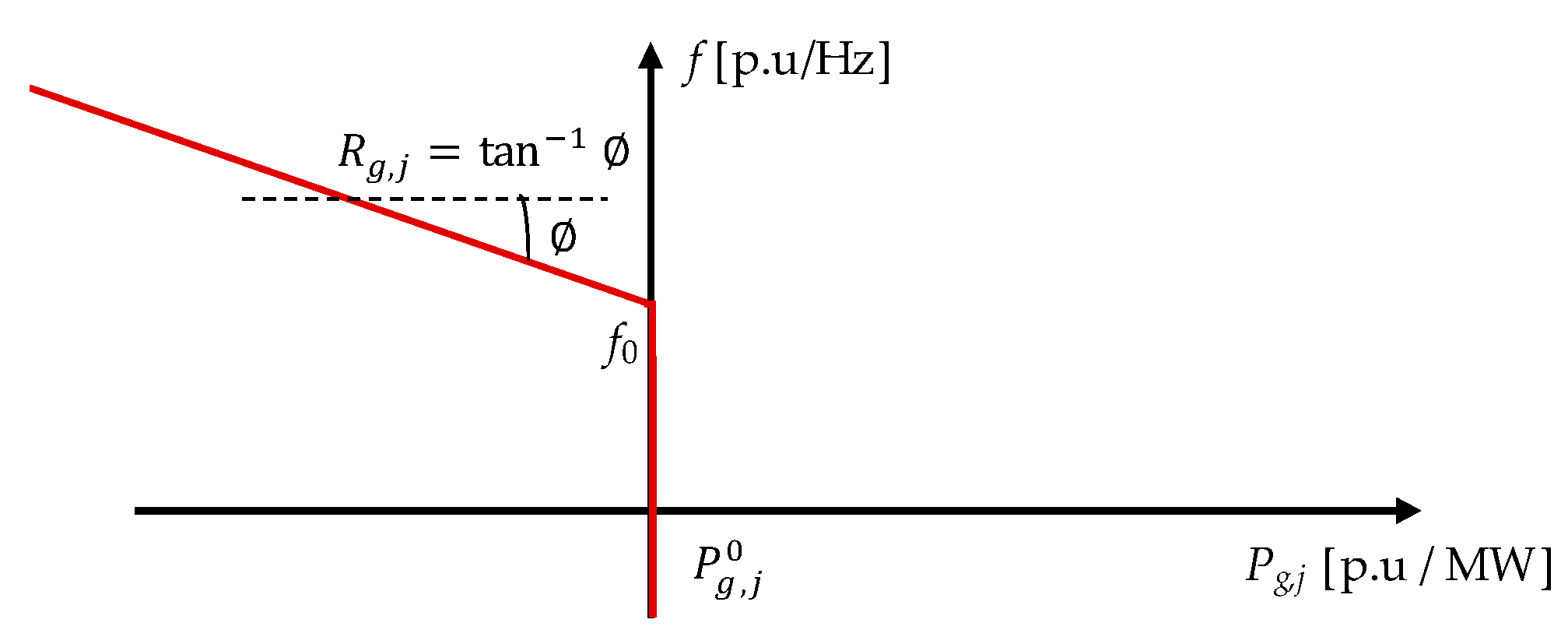
2.1.2. The RES Generator Model

Traditionally, the RES generating units are set to produce at the maximum power available from the primary renewable energy source, maximizing thus the exploitation of the clean and cheap energy source. However, they can be exploited to participate in stabilizing the frequency of a newly formed island in case of emergency, similarly to how the synchronous generators are used. Thus, a linear P-f response law can be imposed to the RES generating unit by adding an additional real power signal to the reference signal provided by the Maximum Power Tracking (MPT) that modifies the reference signal according to the imposed linear P-f response law, and, thus, according to the frequency measurement at the terminals of the RES plant. With respect to the synchronous generator model, a significant difference appears: since it is exploited at maximum available power from the primary source, the RES generator cannot increase its power; this means that the RES generating unit can only respond to over-frequencies.
Figure 2 shows the resulting linear P-f response law for the jth RES generating unit. Here, the significance of the physical quantities is the same as in Figure 1. Mathematically, the model shown in Equations (1)–(4) still holds except for the calculation of the regulating energy. Thus, substituting index i with j in Equations (1)–(4) and rewriting Equation (2) as (5), the model is fully described.
e g , j = { P g , j n R g , j · f 0 if   Δ I < 0   0 if   Δ I > 0
It is clear from Equation (5) that in case of under-frequency (positive imbalance) the regulating energy e g , j is null and thus it will not be included in the total regulating energy of the system. Moreover, according to Equation (1) the RES will not respond to the positive imbalance, so its final real power output will be equal to the initial one. In case of over-frequency (negative imbalance), according to Equation (5) the regulating energy e g , j is available and the RES generating unit behaves as a synchronous generator.

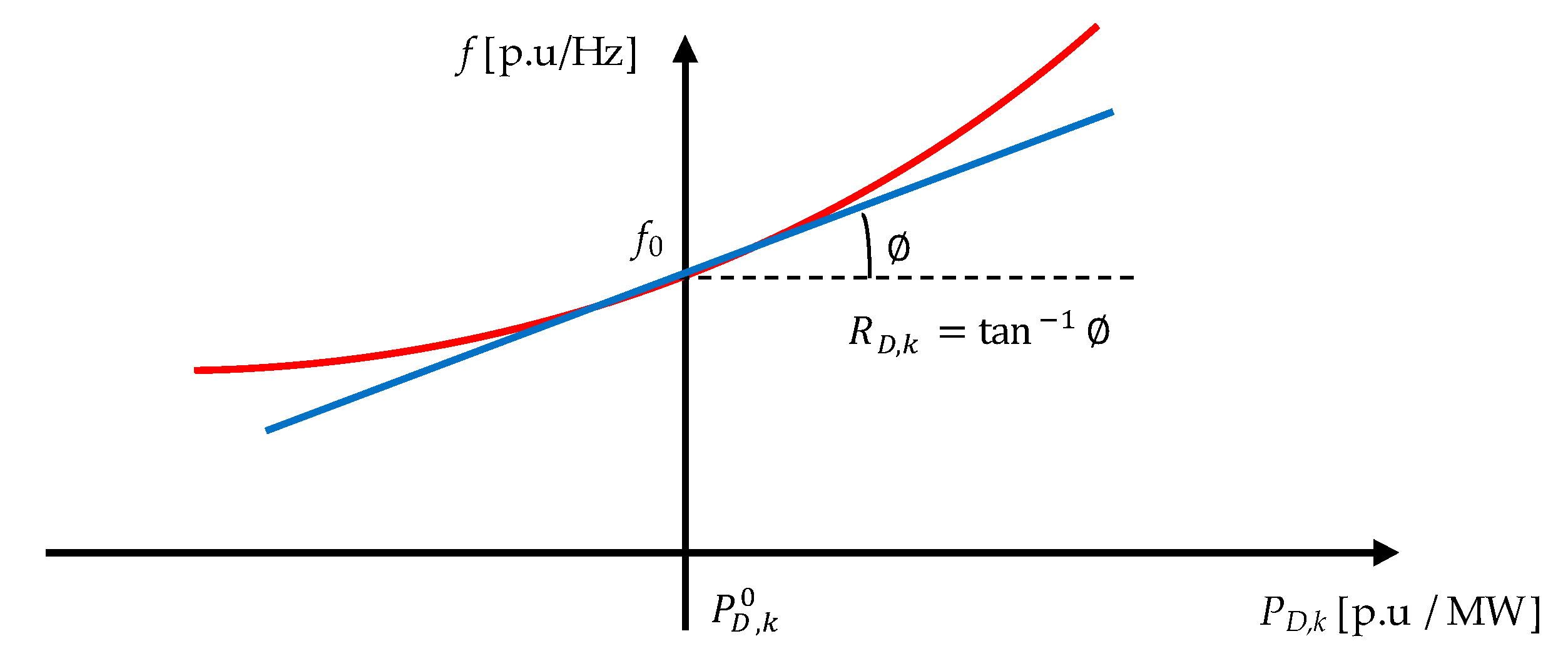
2.1.3. The Demand Response Model

In general, according to [30] the demands are characterized by a natural P-f response. Figure 3 shows, with red line, such a response for demand k, initially absorbing the real power P D , k 0 . As one can see, the response is generally non-linear. However, since a feasible operation of the islanded network implies a final frequency close to the nominal one, i.e., to f 0 , a linearization around the initial operating point of the load (at f 0 ) is feasible. Thus, the blue line is obtained and the demand response model becomes analogous to the synchronous generator frequency response model. The main difference stands in the complementarity of the response to frequency variation: in case of over-frequency the demand increases while the generation output decreases (see Figure 1 and Figure 2), and vice-versa in case of under-frequency. The model Equations (1)–(4) still holds but this difference needs to be considered. Thus, the demand response model is described by Equations (3), (4) (6) and (7).
P D , k 1 = P D , k 0 Δ P D , k
Δ P D , k = Δ I · e D , k e t o t  
e D , k = P D , k 0 R D , k · f 0

2.2. Basic Optimization Model

The goal of the proposed optimization problem is to minimize the shedding actions, i.e., the disconnection of loads and generators, while assuring that the final frequency in the islanded network remains inside acceptable bounds. In doing this, an economic framework has been formulated: the users of the electrical network, i.e., the power plants and/or the demands, (i) can chose to provide emergency frequency restoration services and they are remunerated at a settled price if they are shed or, (ii) can chose not to provide these services thus, their supply becomes a priority and disconnecting them implies a very high cost for the System Operator. Under these circumstances, the minimization of the shedding actions becomes an economical objective, mathematically expressed as the following objective function (OF):
min C s h e d _ g e n + C s h e d _ l o a d
where C s h e d _ g e n is the total cost for shedding the generation, while C s h e d _ l o a d is the total cost for shedding the demand. The two terms of Equation (8) are:
C s h e d _ g e n = i S G Y i · C S G , i · P g , i 0 + j R E S _ 1 Y j · C R E S _ 1 , j · P g , j 0 + l R E S _ 2 Y l · C R E S _ 2 , l · P g , l 0
C g e n _ l o a d = k L O A D S Y k · C D , k · P D , k 0
In the above equations S G is the set of synchronous generators in the islanded network, R E S _ 1 is the set of frequency responsive RES generators in the islanded network, i.e., the ones modeled according to Section 2.1.2, R E S _ 2 is the set of frequency unresponsive RES generators in the islanded network, i.e., the ones operated in the traditional way i.e., at constant power output, while L O A D S is the set of the demands in the islanded network. Further, Y i ,   Y j ,   Y l and Y k are binary variables quantifying the shedding status of the synchronous generators, RES generators and demands, respectively; if they are equal to 1 then the user is disconnected, otherwise they are equal to 0. Parameters C S G , i ,   C R E S _ 1 , j ,   C R E S _ 2 , l and C D , k are the costs associated with the shedding of the synchronous generators, RES generators and demands, respectively. In order to distinguish between the network users providing or not emergency frequency restoration services the costs of shedding the latter are assumed to have values much higher than the former.
The OF is subject to the constraints described as follows. First, the three frequency response models are put together in order to determine the final real power outputs of the network’s components and the final system frequency. Since only the synchronous generators, the frequency responsive RES generators and the demand change their outputs, we have:
P g , i 1 = P g , i 0 + Δ P g , i ,   i S G
P g , j 1 = P g , j 0 + Δ P g , j ,   j R E S _ 1
P D , k 1 = P D , k 0 Δ P D , k ,   k L O A D S
where, according to Equations (1b) and (6b):
Δ P g , i = Δ I · ( 1 Y i ) ·   e g , i e t o t ,     i S G
Δ P g , j = Δ I · Y j * · e g , j e t o t   ,   j R E S _ 1
Δ P D , k = Δ I · ( 1 Y k ) · e D , k e t o t   ,   k L O A D S
In the above, Equations (1a) and (6a) are repeated for consistency. The real power imbalance, Δ I , resulting from the disconnection of the analyzed network from the main power system and the application of the shedding actions is defined as:
Δ I = k L O A D S ( 1 Y k ) · P D , k 0 + P l o s s 0 { i S G ( 1 Y i ) · P g , i 0 + j R E S _ 1 ( 1 Y j ) · P g , j 0 + l R E S _ 2 ( 1 Y l ) · P g , l 0 }
where P l o s s 0 is the real power losses at the moment of island formation. It can be determined from the real power imbalance of the network considering the total power exchanged by the analyzed network with the main power system, P e x c h , as:
P l o s s 0 = i S G P g , i 0 + j R E S _ 1 P g , j 0 + l R E S _ 2 P g , l 0 k L O A D S P D , k 0 + P l o s s 0 P e x c h
In Equation (11b) a new binary variable, Y j * , has been introduced with the goal of modeling the piecewise linear P-f response law of the RES generators (see Figure 2). Thus, this variable is 1 in case of negative imbalance, and 0 otherwise. Two conditions need to be simultaneously satisfied in order to have   Y j * = 1 : (i) the jth generator is connected, i.e., 1 Y j = 0 , and (ii) the imbalance Δ I < 0 . While the first condition is mathematically obvious, the second one is harder to represent. For this purpose, another binary variable X j is used: it is 1 if the imbalance is negative, and 0 otherwise. Mathematically, this can be formulated as:
0.0001 · M j X j 1000 · M j ,     j R E S _ 1
where, M j is the maximum value between 0 and Δ I . This variable is thus determined using the well-known linear model of the “maximum” function:
Δ I M j ,     j R E S _ 1
0 M j ,     j R E S _ 1
M j Δ I + | Δ I 0 | · ( 1 θ j ) ,     j R E S _ 1
M j 0 + | Δ I 0 | · ( θ j ) ,     j R E S _ 1
where θ j is an additional binary variable and Δ I 0 is a parameter equal to the imbalance at island formation and before the application of the shedding actions.
The set of Equation (15) work as follows. If Δ I is positive then, between Equations (15a) and (15b), the latter is more stringent and forces M j to be higher or equal than zero. In Equation (15c) this is possible only if binary variable θ j is null: since the goal of the algorithm is to keep the frequency value close to nominal, the optimization problem tends to reduce the imbalance with respect to the initial one, thus | Δ I 0 | is higher than | Δ I | and Equation (15c) will define a reasonable positive upper bound for M j . With θ j = 0 , Equation (15d) combined with Equation (15b) will limit M j to be both higher or equal than and lower or equal than zero in the same time: it follows that M j = 0 . In contrast, when Δ I is negative Equation (15a) forces M j to be greater or equal than Δ I , a positive value. Therefore, according to Equation (15d) binary variable θ j must be equal to 1; hence, Equation (15c) will force M j to be lower or equal than Δ I and, so, in combination with Equation (15a) it follows that M j = Δ I .
It is now easy to understand the behavior of Equation (14). When Δ I is positive, M j is zero and Equation (14) becomes 0 X j 0 , thus X j = 0 . When Δ I is negative, M j = Δ I , a real positive number. Writing (14) in a raw form, i.e., without the coefficients multiplying M j , X j would be equal to M j . Thus, the raw form of (14) needs to be relaxed to force X j to be one: as the value of Δ I is discrete and depends on the active powers of the loads and generators—see Equation (12), it results it cannot be lower than the minimum of these powers so it will be, in the worst case scenario, a few kW, i.e., 10−3 MW (typical value of household loads); at maximum, Δ I can take values of tens of MW (typical installed load in distribution networks) or hundreds of MW (typical load for small areas of the transmission network). Therefore, multiplying M j with 0.0001 on the left guarantees a strictly positive and sub unitary lower limit for X j while multiplying M j with 1000 on the right guarantees a strictly positive and over unitary upper limit for X j : thus, binary variable X j can only be equal to one when Δ I is negative.
The binary variable Y j * is determined by the “logical AND” condition between X j and 1 Y j . This variable is thus determined using the well-known linear model of the “logical AND” operator:
Y j * X j + ( 1 Y j ) 1 ,     j R E S _ 1
Y j * X j ,     j R E S _ 1
Y j * ( 1 Y j )   ,     j R E S _ 1
The set of Equation (16) work as follows. If both X j and ( 1 Y j ) are 1, then binary variable Y j * is not limited by Equations (16b,c). However, the right-hand of Equation (16a) is equal to 1 so Y j * is forced to 1. When only one or both X j and ( 1 Y j ) are 0, then the right-hand side of Equation (16a) is 0 or −1, respectively, so Y j * is not limit by Equation (16a). However, either one or both Equation (16b,c) force Y j * to 0.
Further, the total available regulating energy, e t o t , is given by:
e t o t = i S G ( 1 Y i ) · e g , i + j R E S _ 1 Y j * · e g , j + k L O A D S ( 1 Y k ) · e D , k
Equations (10), (11) and (14)–(17) are completed by Equations (3) and (4) to obtain the complete representation of the frequency response of the islanded network. Furthermore, additional constraints are necessary to guarantee the security of the islanded network. First, the real power capability constraint for the regulating generators:
( 1 Y i ) · P g , i M I N P g , i 1 ( 1 Y i ) · P g , i M A X ,     i S G
( 1 Y j ) · P g , j M I N P g , j 1 ( 1 Y i ) · P g , j 0   ,     j R E S _ 1
where P g , i M I N / P g , j M I N and P g , i M A X are the active power limits of the frequency responsive generators. For the RES generators the actual production P g , j 0 is used as the maximum limit as they are producing at the maximum power available from the primary energy resource.
Constraints similar to Equation (18) need to be added for the frequency responsive loads in order to assure that the final value of the demanded power, P D , k 1 , is null when the demand is disconnected:
0 P D , k 1 1000 · ( 1 Y k ) · max k L O A D S ( P D , k 1 ) ,       k L O A D S
where number 1000 was introduced to assure a high enough upper margin for the frequency response of each demand.
Following are the frequency reserve bands required to mitigate future variation of the load:
B + τ · k L O A D S P D , k 1
B τ · k L O A D S P D , k 1
where B + and B are the upward and downward system’s frequency reserve bands, respectively. Parameter τ 0 is a user-defined constant quantifying the fraction of the load to be covered by the frequency reserve bands during island operation. Thus, the quantity on the right-hand side of Equation (20) represents the expected long-term variation of the load in islanding conditions. The frequency reserve bands are given by:
B + = i S G { ( 1 Y i ) · P g , i M A X P g , i 1 }
B = i S G { ( 1 Y i ) · P g , i M I N P g , i 1 } + i R E S _ 1 { ( 1 Y j ) · P g , j M I N P g , j 1 }
Finally, the steady-state operation frequency limits are given by:
f M I N f 1 f M A X
where f M I N and f M A X are the minimum and maximum frequency steady-state operation limits, respectively. The value of f 1 is given by Equations (3) and (4) which are considered as constraints of the OF.
Thus, the proposed optimization model is formed of the OF (8) constrained to Equations (3), (4), (10), (12), (14)–(22). In brief, the model is designed to find the set of optimal demand/generation shedding actions, i.e., the optimal set of values for the binary variables Y i ,   Y j ,   Y l and Y k , that minimizes the total cost of shedding (maximizing, thus, implicitly the supplied load) but also assures that (i) the final steady-state frequency is inside acceptable limits—Equation (22); (ii) the regulating generators capabilities are satisfied—Equation (18) and (iii) there is enough regulation margin to assure the long term frequency stability of the network—Equation (20). Finally, it should be noted that all the equations that form the optimization model are linear, except constraint Equation (11) which introduces non-linearity in the model due to the multiplication of e t o t with the frequency response of the real power of the network’s load and generators ( Δ P g , i , Δ P g , j and Δ P D , k ). The presence of this non-linearity determines the optimization model be a MINLP problem.

2.3. Advanced Optimization Model: Decomposition Model

The main disadvantage of the Base Model stands in its non-linearity: adopting a deterministic method to solve the problem (generally, a branch-and-cut method) will determine the exponential increase of the computation time with the size of the problem; it is therefore highly probable that the computation time will exceed the stringent tolerances required by a real-life implementation. In order to mitigate this, a procedure that gradually filters through the sheddable users in order to provide to the MINLP a substantially reduced set of variables is proposed. Figure 4 illustrates the flowchart of the main steps of the proposed procedure: (i) first, a simplified and linear version of the MINLP model is solved in quick times in order to have a decent estimation about the users the Base Model would shed then, (ii) this information is used together with the frequency-response capabilities and shedding costs to obtain a reduced set of sheddable users and, thus, drastically reduce the number of variables and constraints (second block in Figure 4), for the non-linear Base Model (third block in Figure 4). While the Base Model was already introduced previously, the first two blocks of Figure 4 are further detailed.

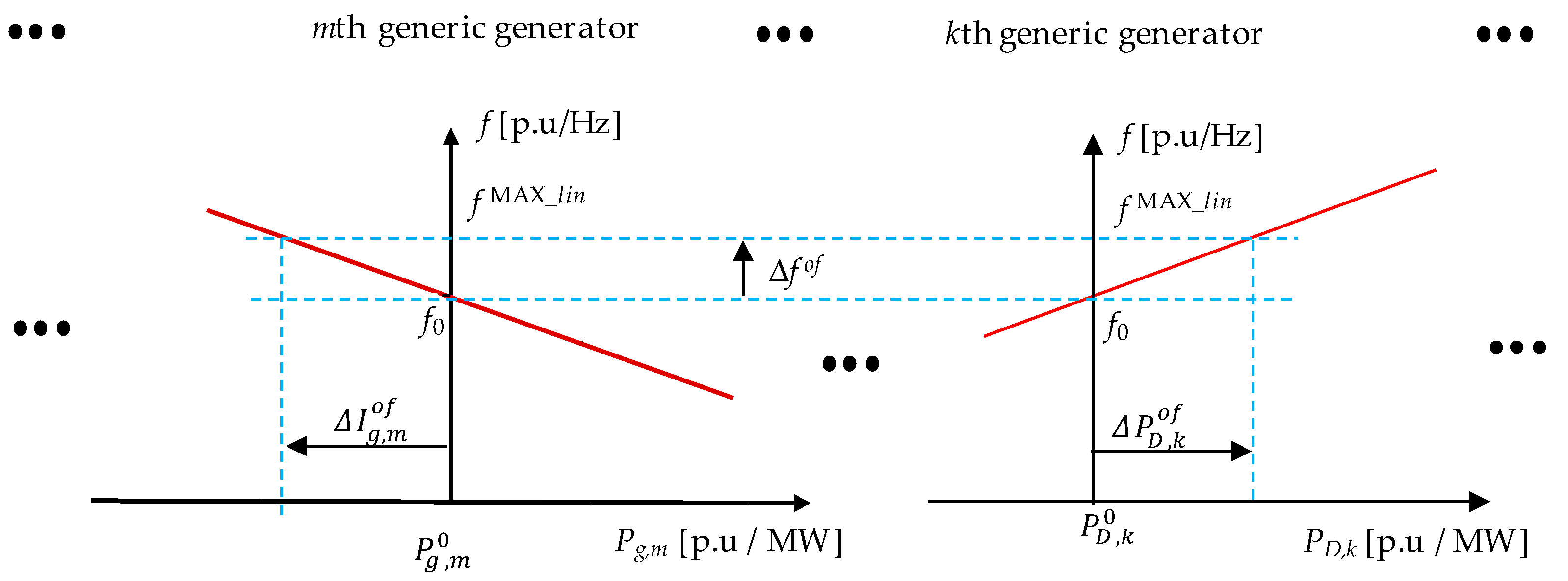
2.3.1. The Linear Optimization Problem

The goal of this optimization problem is the same as the one of the Base Problem, therefore the same OF Equation (8) is used. The difference stands in the formulation of the constraints. In the base problem the non-linearity is given by the set of Equation (11) which are required to explicitly calculate the final real power and network’s frequency in islanding conditions. Here, a simplified constraint is designed to implicitly consider this aspect and neglect the variables and constraints associated with the explicit calculation (the ones with superscript “1”). In order to clearly understand, the new constraint is explained in few logical steps.
First, a minimum and maximum frequency limits are defined, i.e.,   f M A X _ l i n and f M I N _ l i n , respectively. Since the linear model represents an approximation, these limits are slightly higher than the ones used by the Base Model, i.e., f M A X and f M I N , respectively. Then, it is considered that no shedding action occurs during islanding and the total regulating energy of the network for over-frequency, e t o t o f , and under-frequency, e t o t u f , is calculating using Equation (17) where all Y i and Y k are considered equal to 0 and all Y j * are considered 1 for over-frequency or 0 for under-frequency (see Figure 2 or Equation (5) for clarification). Then, e t o t o f and e t o t u f are used in combination with Equation (4) to calculate the theoretical imbalance the network’s power plants should compensate, i.e., Δ I o f and Δ I u f , respectively, in order to bring the frequency at f M A X _ l i n and f M I N _ l i n , respectively. Mathematically, then:
Δ I o f = Δ f o f e t o t o f
Δ I u f = Δ f u f e t o t u f  
where Δ f o f = f M A X _ l i n f 0 and Δ f u f = f M I N _ l i n f 0 .
This calculation is illustrated in Figure 5 only for the over-frequency case: the under-frequency case is analogous. Here, only the mth generator and kth demand are considered. Without losing the generality, the mth generator is considered a conventional unit and Δ I g , m o f is the part of Δ I o f provided by this unit. To be noted that when Δ I o f and Δ I u f are determined, the capability of the generators is considered.
Then the fraction of Δ I o f and Δ I u f occupies from to the total available frequency-responsive generated power is determined:
μ o f = Δ I o f i S G P g , i 0 + i R E S _ 1 P g , j 0
μ u f = Δ I u f i S G P g , i 0  
Finally, as the slopes of both the frequency-responsive generators and demands are generally very similar (a few per cents) it is reasonable to consider that in the presence of the shedding actions, the frequency-response characteristic of the network changes, averagely, very little in terms of slope ( Δ P / Δ f ); on the contrary, the regulating capacity can change substantially. Therefore, it is reasonable to assume that coefficients μ o f and μ u f do not change substantially when shedding actions are performed. Thus, considering them constants, the following constraint on the real power imbalance after islanding and application of the shedding actions, Δ I , can be formulated:
μ o f · { i S G ( 1 Y i ) · P g , i 0 + i R E S _ 1 ( 1 Y j ) · P g , j 0 } Δ I μ u f · { i S G ( 1 Y i ) · P g , i 0 }
where Δ I is given by Equation (12).
Since μ o f and μ u f are determined by f M A X _ l i n and f M I N _ l i n , it results that Equation (25) limits Δ I to values that will not violate the defined frequency limits once the frequency-response of the network components is stabilized. Therefore, constraint Equation (22) is now implicitly guaranteed for the relaxed limits f M A X _ l i n and f M I N _ l i n , respectively, and constraints Equations (10), (11), (14)–(19) and (22) are no longer necessary. However, so as to guarantee a longer-term feasibility of the network, the constraints on the regulating bands available after islanding stabilization, i.e., Equations (20) and (21) in the Base Model, are still necessary. Since the final output of the generators can no longer be determined, these constraints are reformulated as:
B l i n + Δ I + τ · { k L O A D S P D , k 0 l R E S _ 2 ( 1 Y l ) · P g , l 0 }  
B l i n Δ I τ · { k L O A D S P D , k 0 l R E S _ 2 ( 1 Y l ) · P g , l 0 }  
where,
B l i n + =   i S G { ( 1 Y i ) · P g , i M A X P g , i 0 }
B l i n =   i S G { ( 1 Y i ) · P g , i M I N P g , i 0 } + i R E S _ 1 { ( 1 Y j ) · P g , j M I N P g , j 0 }
It should be noted that the presence of Δ I in Equation (26) has the role to implicitly consider the frequency response of the generators after islanding.
To summarize, the Mixed-Integer Linear Programming (MILP) problem that constitutes the simplified model is composed of the OF Equation (8) constrained by Equations (4), (25)–(27).

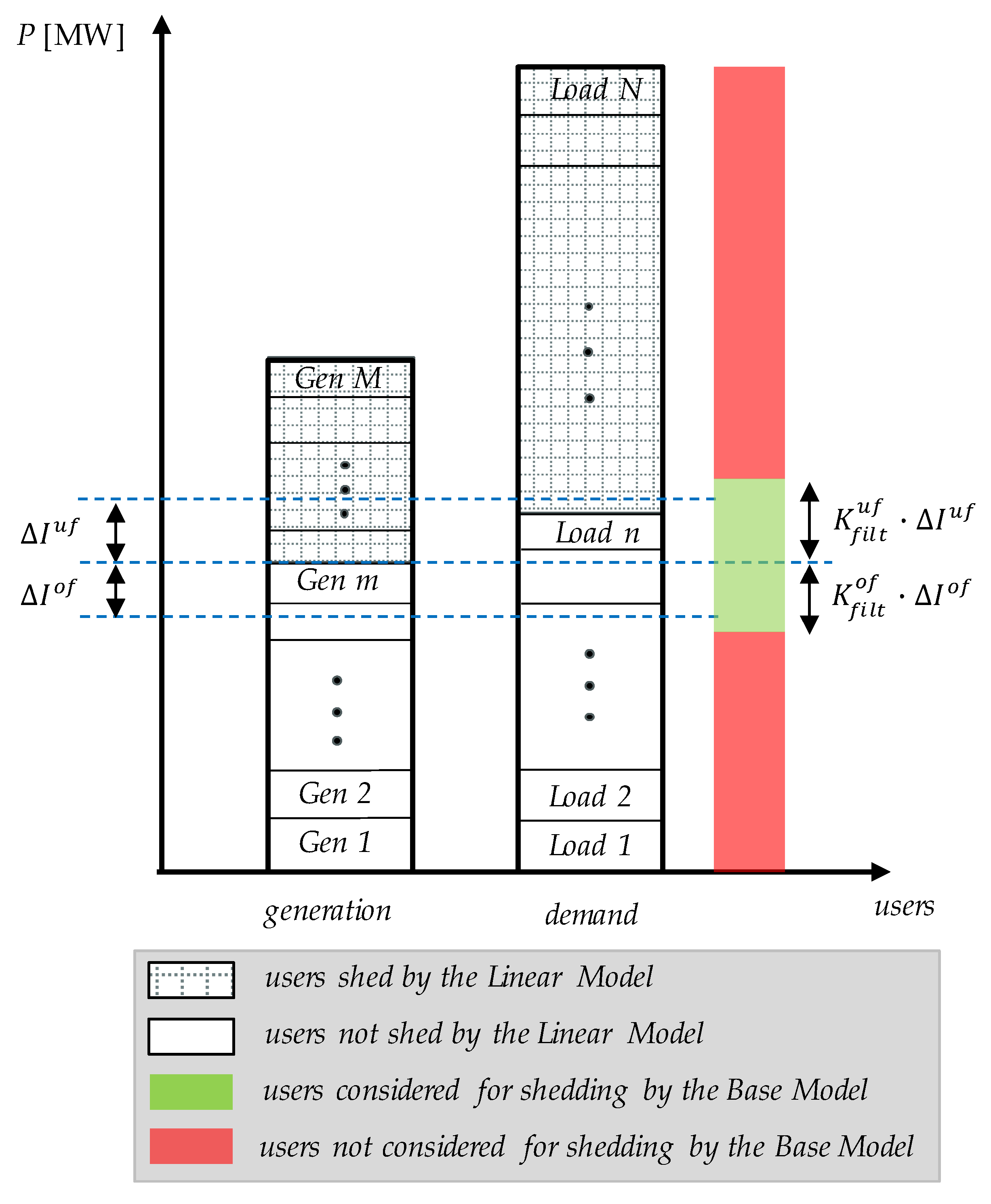
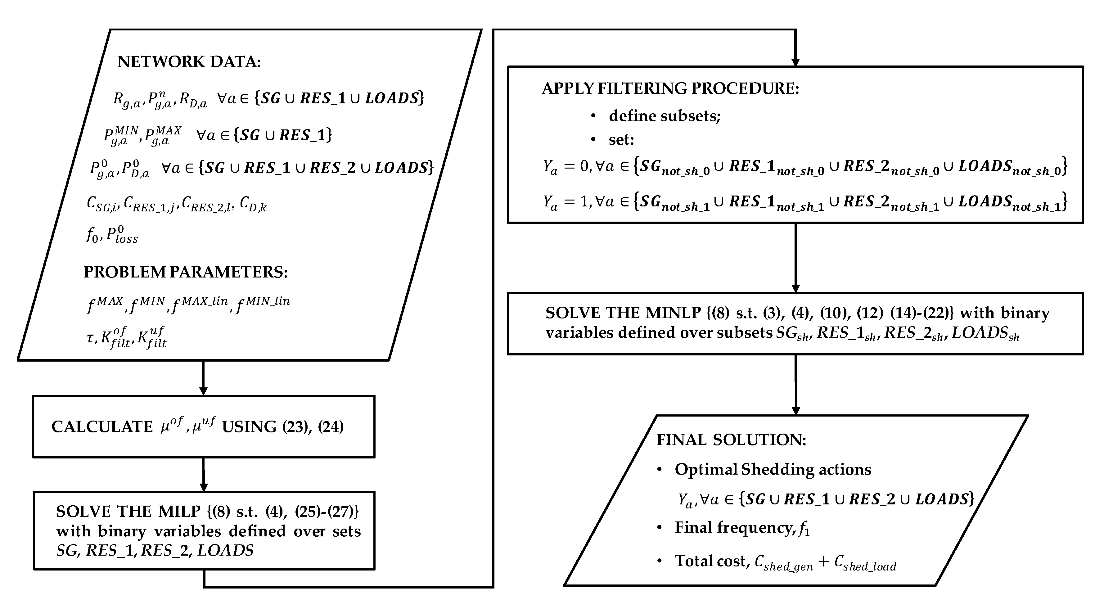
2.3.2. The Filtering Procedure

The solution obtained by solving the Linear Model can be depicted graphically in Figure 6 where the cumulated initial real power of the generators and demands is represented; moreover, the generators and the demands are sorted according to the shedding status given by the solution of the Linear Model. Then, both the users shed and not shed by the Linear model are classified independently according to the shedding costs in ascending order (e.g., from Gen 1 to Gen m, and Load 1 to Load n in Figure 5); the users of equal costs are further sorted according to their frequency-response performances: from the highest to the lowest regulating energy. With the users classified as described, it is clear from Figure 5 that the users outside the [ Δ I o f ,   Δ I u f ] area are clearly sheddable (the area above Δ I u f ) or clearly not sheddable (the area bellow Δ I o f ). However, since the Linear Model provides an implicit answer, the status of the few users in the area inside [ Δ I o f ,   Δ I u f ] is not clear.
Thus, an explicit verification of the security constraints is required to determine exactly which users in the [ Δ I o f ,   Δ I u f ] area to shed: for this, the Base Model is executed by setting (i) the binary variables ( Y i ,   Y j ,   Y l and Y k ) corresponding to the users in the area above Δ I u f to 0; they form the subsets S G n o t _ s h _ 0 , R E S _ 1 n o t _ s h _ 0 , R E S _ 2 n o t _ s h _ 0 , L O A D S n o t _ s h _ 0 of the sets S G , R E S _ 1 , R E S _ 2 , L O A D S , (ii) the binary variables ( Y i ,   Y j ,   Y l and Y k ) corresponding to the users in the area bellow Δ I o f to 1 and; they form the subsets S G n o t _ s h _ 1 , R E S _ 1 n o t _ s h _ 1 , R E S _ 2 n o t _ s h _ 1 , L O A D S n o t _ s h _ 1 of the sets S G , R E S _ 1 , R E S _ 2 , L O A D S , (iii) the binary variables ( Y i ,   Y j ,   Y l and Y k ) corresponding to the users in the area [ Δ I o f ,   Δ I u f ] area as free variables; they form the subsets S G s h , R E S _ 1 s h , R E S _ 2 s h , L O A D S s h of the sets S G , R E S _ 1 , R E S _ 2 , L O A D S . The union of the three subsets for each type of network’s user is equal to the full set, i.e., S G = S G n o t _ s h _ 0 S G n o t _ s h _ 1 S G s h , R E S _ 1 = R E S _ 1 n o t _ s h _ 0 R E S _ 1 n o t _ s h _ 1 R E S _ 1 s h , R E S _ 2 = R E S _ 2 n o t _ s h _ 0 R E S _ 2 n o t _ s h _ 1 R E S _ 2 s h and L O A D S = L O A D S n o t _ s h _ 0 L O A D S n o t _ s h _ 1 L O A D S s h . Thus, mathematically, the Base Model is run after the filtering procedure with the binary variables pertaining to only the subsets S G s h , R E S _ 1 s h , R E S _ 2 s h , L O A D S s h , instead of the full sets. Obviously, the resulting redundant constraints are eliminated from the Base Model.
Finally, since the Linear Model guarantees implicitly the satisfaction of the constraints of the Base Model, it is possible to enlarge the area of selected sheddable users to [ K f i l t o f · Δ I o f ;   K f i l t u f ·   Δ I u f ] , where K f i l t o f and K f i l t u f are two user-defined coefficients, higher or equal to 1.
To clearly understand how the complete Advanced Optimization Model is applied, Figure 7 depicts a detailed flow-chart of the algorithm.

3. Results

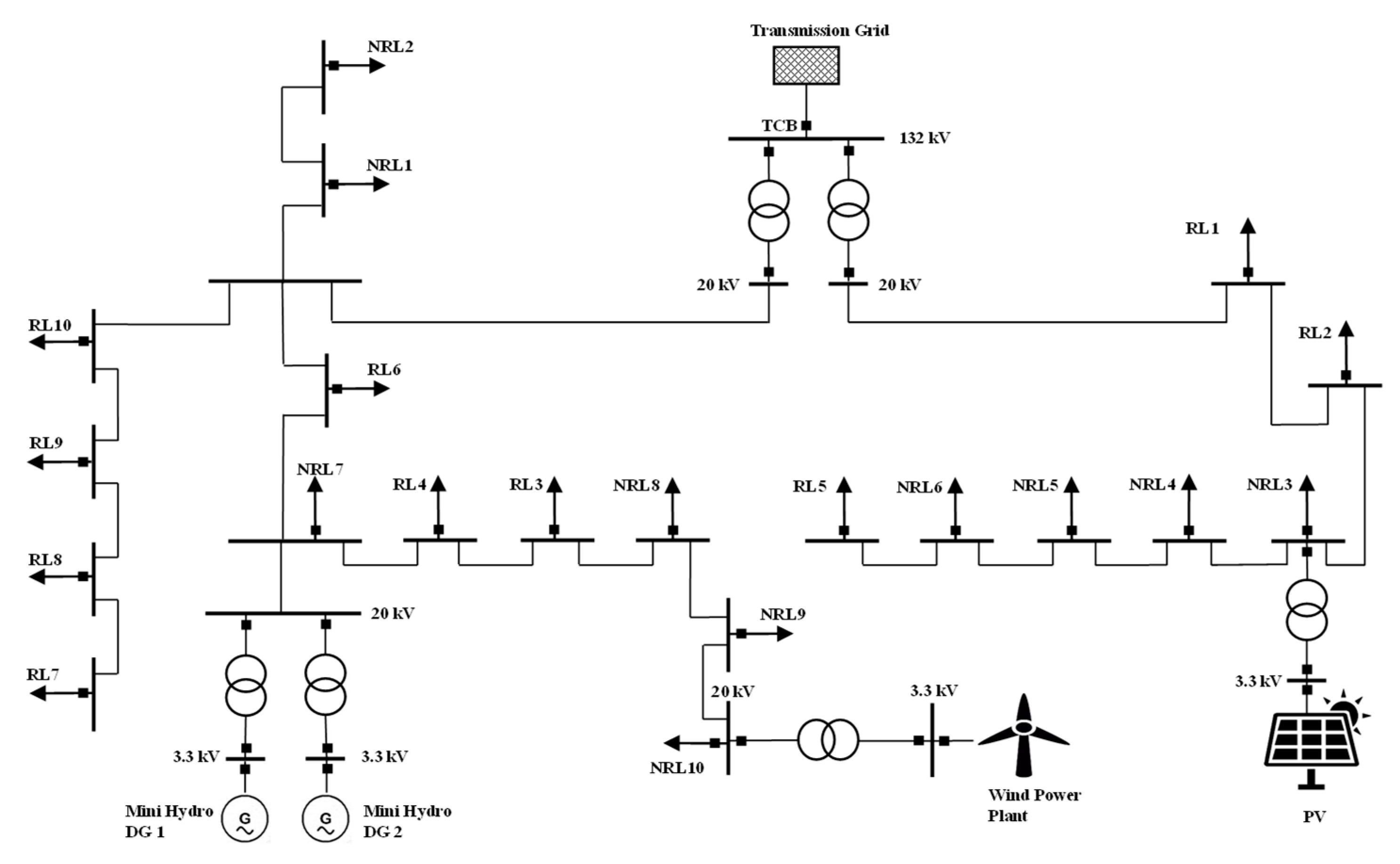
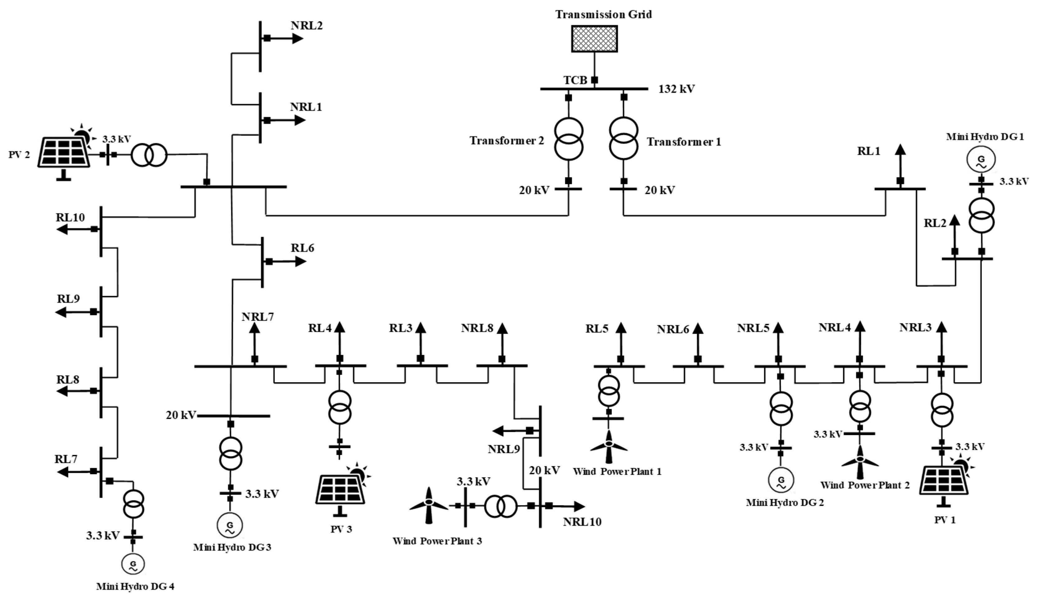
3.1. Test Network-Base Configuration

The proposed optimization models have been implemented in GAMS 24.0.2 modeling environment [31], a software specially designed to represent and solve optimization problems. The Basic Model was solved using the LINDOGLOBAL 7.0.1 solver [32]. The solver uses a branch-and-bound method to find the solution to the problem. The Linear Optimization Problem of the Advanced Model was solved using the CPLEX 12.5 solver [33]. The solver uses a branch and cut method which solves a series of continuous Linear Programing subproblems with a state-of-the-art dual simplex algorithm developed by IBM. All the employed methods are deterministic, so the disadvantages related to the heuristic method are mitigated. Moreover, in order to guarantee that the best possible feasible solution is found, the optimality gaps of the optimization methods where set to the smallest values allowed by the software. Last, but not least, the simulations were carried on a PC equipped with an Intel® Core™ i5-2500 @3.3 GHz processor, 8 Gb RAM and 500 Gb HDD was used.
The proposed procedures have been tested on the MV distribution network depicted in Figure 8. The electric parameters and the network configuration are taken from [34] while the network generating units and demands has been set to represent a distribution network with a basic degree of penetration of distributed generation. This system is a 20-kV distribution network which is connected to the transmission grid via two units of step-down transformers (132/20 kV), rated 32 MVA each.
In Figure 8 there are 4 generation plants: two Mini-Hydro Plants producing 10 MW each, one Wind Power Plant producing 10 MW and one Photovoltaic Plant producing 5 MW. Each of these plants is made of 10 identical and sheddable generating units producing equal amount of power. While the hydro-generators are synchronous generators, so they form the set SG and they traditionally provide frequency-response due to their mechanical inertia, among the RES plants the wind generators were selected to form the set of frequency-response renewables, i.e., RES_1, while the photovoltaic generators were included in set RES_2, so they do not provide frequency response. The slopes of the frequency response characteristics of the generators, i.e., the R g coefficients, were randomly set in the range (0.06–0.09) according to a normal distribution; this range of values are typical for the generators in operation nowadays [30]. Further, there are 20 load plants connected at the buses of the network (the RLs (Restorative Loads) and NRLs (Non-Restorative Loads), in Figure 8). Each load plant is made of 10 identical and sheddable demands of which power consumption is reported in Table 1. Moreover, Table 1 shows the frequency-response characteristics; these numbers were set according to the typical frequency-response characteristics of residential loads as indicated in [30].
The model of the network with the above characteristics has been implemented in the DIgSILENT 2018 [35] software, which was used to perform both steady-state calculations (power flows) and dynamic analysis. For the latter, standard models provided by the DIgSILENT library have been used for the generators and the demands. The models of the wind generators have been slightly modified to accommodate the linear frequency-response characteristic imposed to these plants: the active power reference of the electronic converters of these units was changed such to follow the P-f law; here, the set-point defined by the MPT is used as reference (the P g f 0 point in Figure 2).
Figure 9 illustrates the global characteristics of the network in terms of active power in the initial operating conditions of the grid (connected to the main network). A power flow calculation has been executed and the resulted power losses in the network are 1.19 MW while the test network absorbs 19.29 MW from the external grid, number which also represents the imbalance of the test network in case of islanding without taking any shedding actions; this imbalance is almost equal to the production of the generators in the grid and about 35% of the total load in the grid. In fact, the dynamic simulation of the islanding of the grid without shedding (opening of the TBC breaker, see Figure 8) shows that the frequency stabilizes at 48.4 Hz, as depicted in Figure 10 where the islanding occurs at t = 5 s. Comparing these values to the limits defined for the protection systems of the RES plants, i.e., 47.5–51.5 Hz (see, e.g., [36]) it results is very critical: it is close to the minimum limit so any further disturbance in the islanded network risks to leave the island unsupplied.
It is clear from the above that the proposed optimization model is required in order to reduce the imbalance in case of island formation and contain the value of the frequency, reducing thus substantially the risk of not supplying the remaining demand in the island. To run the algorithms, it is necessary to first set the shedding costs for the generation and demand units. For this, first the network’s users were divided into frequency-restoration service providers and non-providers. The providers were selected to be the generators in the RES_2 set as they don’t have frequency-response and a part of the demand (the RL loads in Figure 8). The non-providers were selected to be the generators in the SG and RES_1 sets, as they have frequency-response, so keeping them connected is a priority, and a part of the demand (the NRL loads in Figure 8). The prices for shedding the providers has been set according to the prices registered on the Italian Ancillary Service Market [37] where the average price for balancing services is of order of hundreds of €/MWh, while the prices for shedding the non-providers have been set to much higher values than the prices of the providers so to heavily penalize their shedding. Moreover, high priority to maintain the SG generators have been given. The resulted costs are shown in Table 2 and Table 3.

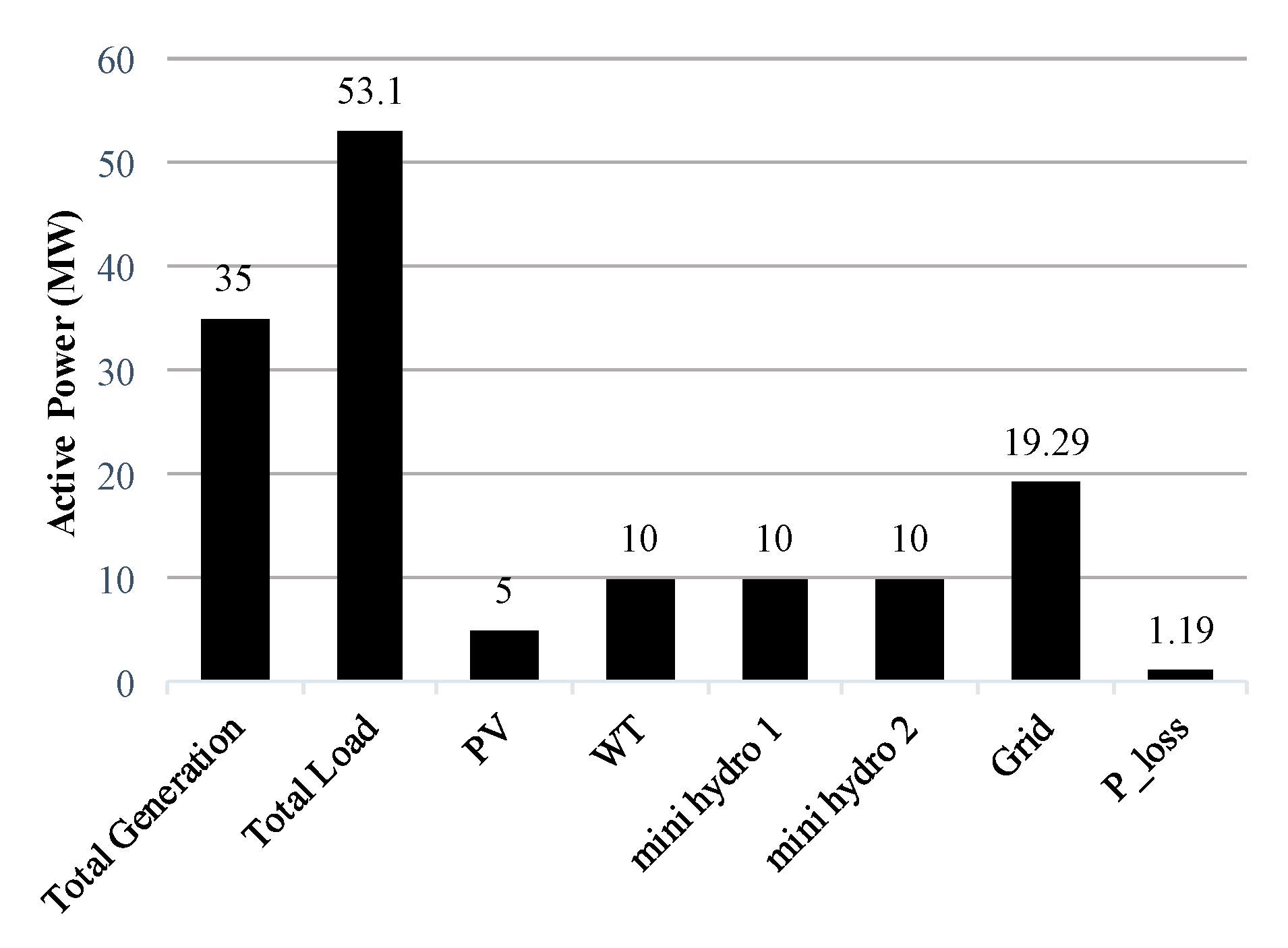
3.2. Results of the Base Configuration

Both optimization algorithms were executed with the following set-up: (i) three configurations for the f M I N f M A X limits of the Basic Model were used, namely: 49.4–50.9 Hz, 49.6–50.6 Hz and 49.8–50.3 Hz, respectively; these configurations were set with the objective of constraining the frequency symmetrically with respect to the nominal frequency and to gradually force the final frequency, f1, in the vicinity of the nominal frequency; (ii) parameter τ was fixed to 0.2; (iii) f M I N _ l i n - f M A X _ l i m limits of the Advanced Model were set as f M I N _ l i n = f M I N 0.4   H z and f M A X _ l i n = f M A X + 0.4 H z ; (iii) coefficients K f i l t o f and K f i l t u f were set to 1.
Table 4 shows the global results of both models in terms of final island imbalance, Δ I , final frequency, f 1 , the total costs of the shedding actions, the shed demand in terms of total number of shed demands and the corresponding total amount of shed power and the computation times. Since the network in its initial state has much more load than generation, therefore under-frequency case, the minimum frequency limit is the critical one, reason why only its value is shown in the table. For the same reason, no generating unit is shed by, thus this information is not shown.
As it can be seen the two algorithms produce similar results: the imbalance and, hence, the final frequency and the total shed load are very close. However, the Advanced Model introduces slightly higher costs but it has the major advantage of converging in considerably faster times. Further, the tightening of the frequency limits decreases the imbalance and, thus, increase the amount and number of shed demand.
Further, it is interesting to note that the final frequency of the island does not reach the limits but is close to them. It could be expected that the limit is reached in the optimal point as the frequency increases with the quantity of shed load so the costs increase accordingly (in other words, increasing the value of Δ I is contrary to minimizing the OF). This does not happen due to the discrete nature of the shed demand.
To test the feasibility of the solution in terms of its actual application, dynamic simulations are carried. The islanding (opening the TBC breaker) occurs at t = 5 s while the shedding actions (opening of breakers of the demands) at t = 5.2 s. A delay of 200 ms was considered in the application of the shedding actions in order to consider the communication delays between island detection and the shedding actions. It could be argued that also the delay associated with the computation time of the optimization models should be considered; this is not the case as the optimization models can be run preventively, in real time, reason why the computation time needs to be as small as possible.
Figure 11 shows the dynamic response of the network’s frequency for the considered cases and for the case when the shedding actions are not applied. As it can be seen, in all the cases when the shedding actions are applied the frequency stabilizes and its transients are well contained when compared to the no-shedding situation. Moreover, the transients resulted from the shedding actions computed by the two Optimization Models are almost identical for all the cases. This validates the simplifications made for the Advanced Model also from the point of view of the transitory response.
Finally, in order to fully validate the model, it is necessary to compare in detail the results of the two models with the actual network behavior. For this reason, Table 5 shows this comparison in terms of final frequency and production of the generating plants: the comparison is provided both in absolute values and relative percentual errors. The results are very similar both between the two optimization models and between the optimization results and the dynamic simulations.

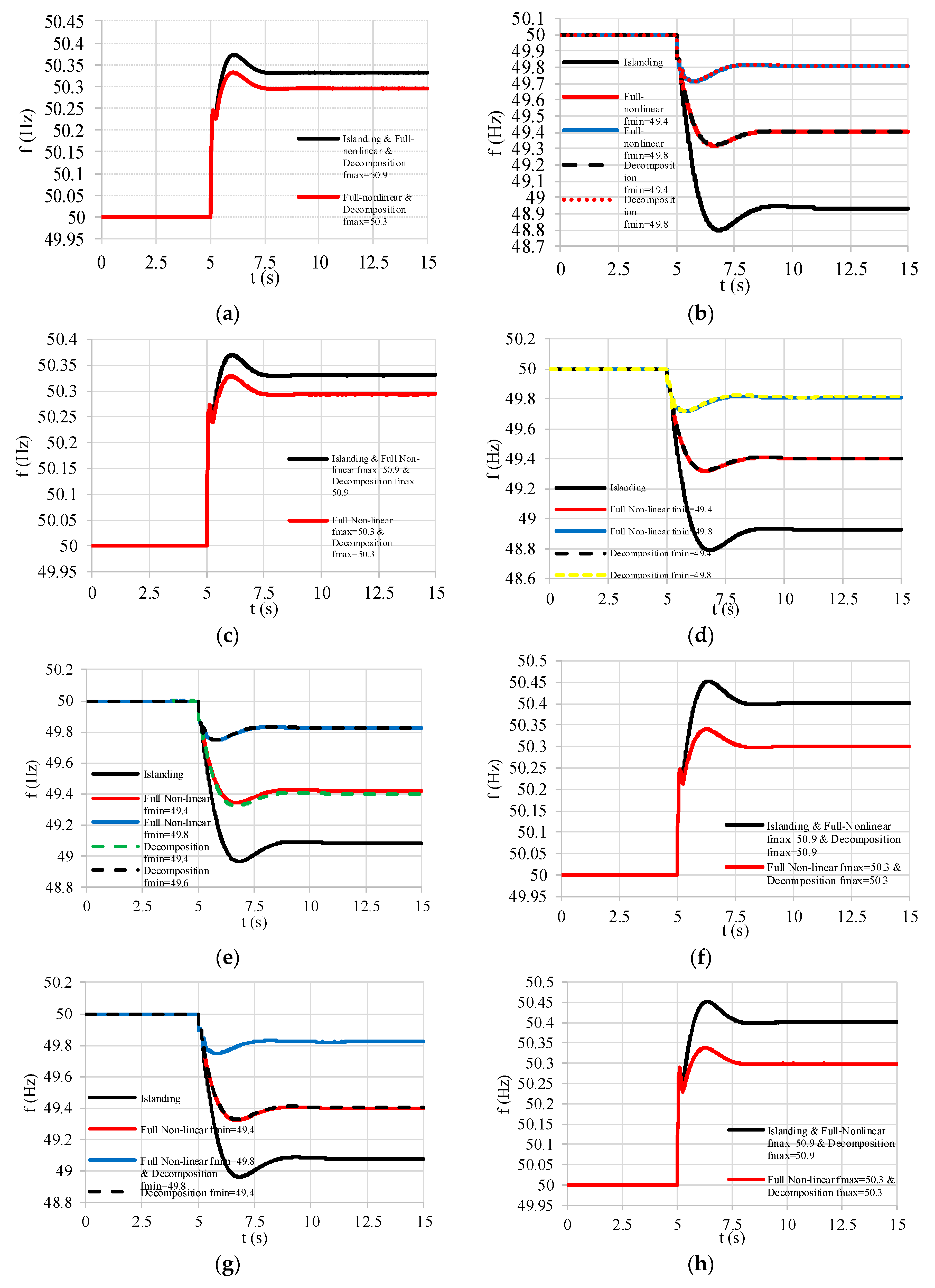
3.3. High Penetration of Distributed Generation Configuration

The previous analyzed network configuration represents a basic low level of distributed generation. In this section additional generation is introduced to generate cases with high level of penetration of distributed generation. In brief, this was done by adding more plants with the same characteristics as the ones previously considered. Moreover, in order to obtain a larger number of possible situations, the generation output and demand power has been varied proportionally to the values of the previous analysis. Figure 12 illustrates the obtained network, while Table 6 shows the main characteristics of the generated scenarios. Additionally, this time the island formation is considered separately, for each transformer (the MV side breakers of both transformers are opened simultaneously) in order to create the following situations: (i) Generation greater than load (share of RES DGs > traditional DGs)—case 4 DN1 and 6 DN2; (ii) Generation greater than load (share of traditional DGs > RES DGs)—case 5 DN1 and 7 DN2; (iii) Load greater than generation (share of RES DGs > traditional DGs)—case 6 DN1 and 4 DN2; and (iv) Load greater than generation (share of traditional DGs > RES DGs)—case 7 DN1 and 5 DN2. In other words, according to Table 6, cases 4–5 and cases 6–7 have the same initial imbalance, total generation and total load for both DNs, separately; only the proportion of the RES plants with respect to the total generation differs.
The optimization models were run with the same set-up as in the previous paragraph, except that only two configurations for the f M I N f M A X limits of the Basic Model have been used, namely: 49.4–50.9 Hz and 49.8–50.3 Hz, respectively. The synthetized results are shown in Table 7 and they represent the same quantities as the ones from Table 4. Depending on the case, only the most stringent frequency limit is reported.
In general, the performance of the models is qualitatively similar to the ones emphasized before. The two models give very similar results, but the Advanced Model tends to shed at marginally higher costs; however, the Advanced Model has the neat advantage of much reduced computation times (e.g., in one of the worst cases, case 6 DN1 fMIN = 49.8 Hz, the Basic Model converges in about 94 s while the Advanced Model in only 2 s). However, with respect to Table 4, here there are some cases of over-frequency, when the generation is higher than the demand (see Table 6). For these cases, without any shedding action the final island frequency is 50.331 Hz and 50.401 Hz, for cases 4-5 DN1 and cases 6–7 DN2, respectively. These values do not violate the maximum limit of f M A X = 50.9 Hz so in these cases, both models determine no shedding actions. When the limit is set to f M A X = 50.3 Hz this limit is marginally violated and both Models shed one generating unit from the RES_2 set for cases 4–5 DN1, and two generating units from the RES_2 set for cases 6–7 DN2, while no load is shed. These minimal actions help to reduce the frequency just below the limit, i.e., to 50.294 Hz and 50.3 Hz, respectively.
Finally, comparing case 4 with 5 and case 6 with 7 for both DNs, independently, one can notice a high degree of similarity between the solutions: this means that the variation of the proportion of RES with respect to the total generation has a small impact on the results.
Figure 13 shows the dynamic response of the frequency of the two DNs for the considered cases and for the case when the shedding actions are not applied. The same settings as in the base network configuration were used. Again, the frequency stabilizes and its transients are well contained in all the cases. Moreover, the transients resulted from the shedding actions computed by the two Optimization Models are almost identical for all the cases.
Table 8 synthesizes the detailed comparison between the optimization model results and the dynamic simulations results: statistical information on the relative errors between the two is given for the final frequency and production of the generating plants. The errors are generally well contained, except in some cases where it gets in the vicinity of 1%. In these cases, they are calculated for small values of the absolute quantities so, in reality, they are still small. Thus, it can be said that the model correctly evaluates the dynamics of the network in terms of frequency response.

4. Discussion

The islanding formation and the application of the shedding actions determined by the proposed models have been tested for the real behavior of the network by performing transient simulations using a proficient software, DIgSILENT 2018. The dynamic models that were used, i.e., the ones present in the standard library of the software, are industry standard and represent realistic models. Therefore, the dynamic simulations are reliable benchmarks. Thus, the fact that the proposed optimization models can accurately match the transient simulations validate them from a practical point of view: these models can be used in real life to optimize the security of the network and reduce the risks of full-network blackouts.
When compared to the methodologies present in literature and reviewed in the “Introduction” section of this paper, the obtained results clearly show the advantages of the proposed approach. When compared to the rough strategies of [19,20,21,22,23,24,25] it is clear that the proposed methodology offers a refined optimal solution: each network’s user is here considered individually and its frequency response modeled correctly; thus, the frequency is pushed towards the defined limits in the same time with the active power imbalance, this determines a minimization of the number of the shedding actions and, hence, of the shedding costs; it is thus possible to accurately control the value of the frequency in the islanded network and, thus, keep it very close to the nominal. These things are not possible using rough strategies: even if the protection relays thresholds are optimized, it will still lead to a not-optimal shedding where the frequency sets in the vicinity of the last activated threshold (to be noted that these thresholds must be set reasonably distant from the nominal frequency of the network to prevent unwanted triggering). Continuing, the proposed method is directly comparable with the approaches proposed in [26,27,28]. Using these approaches, it is possible to obtain very close results (qualitatively identical) with the proposed approach. However, there are important differences that make the current approach the clear winner. Firstly, the previous approaches do not consider, or partially consider, the frequency response of the network components; instead, they use parameter dependent constraints to limit the active power imbalance and obtain the desired effect: as shown in these papers, these parameters are difficult to set and unreliable as they are strongly case dependent: this issue is successfully mitigated here by the accurate representation of the frequency response. Secondly, for similar size to our approach optimization problems, the computation time required by the previous approaches matches the computation time of the Base Model, here proposed: it can reach a couple of minutes. This makes the previous approaches harder to implement on-line: the quality of network’s monitoring would be poor as updates of the network’s state and shedding actions are possible every few minutes. This issue is successfully mitigated here by the well contained computation times of the Advanced Model.
The immediate question is how to apply these models in real life. Clearly, even the short computation times of the Advanced Model are not fitted for an application at island formation: in the presence of high initial imbalance the frequency derivative can be so high that the relay protections would be immediately triggered. Thus, these procedures can be applied preventively, i.e., in normal operation of the network the set of shedding actions can be predetermined with a frequency of a few seconds and immediately triggered in case the islanding occurs. For this purpose, the simplifications introduced by the Advanced Model guarantee a fast computation time, while the Basic Model, applied here with a reduced set of variables, guarantees the accuracy of the solution.
However, the next question can be if such an algorithm is feasible from a practical point of view considering that, historically, unintentional islanding is not a frequent event and that putting in practice such an algorithm requires huge investment into monitoring the network, especially at distribution level. In a future perspective the answer is a sound yes. The power system generation is fast evolving from strongly programmable primary energy resources towards strongly non-programmable, i.e., the RES. The intrinsic uncertainty of the latter type of generation will definitely increase the probability of unintentional islanding. In this perspective, the tool developed in this paper is a much better alternative to the traditional, unoptimized load shedding scheme: it is especially designed to maximize the number of users (generating plants and demands) that remain connected to the islanded grid while the normal and secure island operation is guaranteed.
The proposed model gives also an economical perspective, even if it was formulated in a simple manner. It opens the possibility to emergency ancillary services for the RESs and demand plants, services that are remunerated. Already, at European level, the traditional ancillary services markets are gradually opening to the non-programmable generation and to the demand, with a full market integration in perspective for the near future.
Clearly, the algorithms developed in this paper represent a basic building brick, so they can be furthered evolved. With the capability to tackle the frequency behavior of the islanded network proven, other aspects not considered here can be developed by future research: (i) first, the integration into such a model of the voltage related problems; (ii) secondly, the definition of the optimal islanded area or areas such that the initial imbalance (before the application of the shedding actions) is minimized; and (iii) the presence of other frequency-response capable equipment, like storage.

Author Contributions

Conceptualization, C.B., V.I., A.B. and A.S.; methodology, V.I. and S.A.A.; formal analysis, S.A.A.; resources, A.S., S.G.S. and A.B.; investigation, S.A.A. and V.I.; data curation, S.A.A.; writing—original draft preparation, V.I. and S.A.A.; writing—review and editing, A.S., C.B. and V.I.; supervision, A.S., S.G.S. and A.B.

Funding

This research received no external funding

Conflicts of Interest

The authors declare no conflict of interest.

References

  1. Stock, D.S.; Sala, F.; Berizzi, A.; Hofmann, L. Optimal Control of Wind Farms for Coordinated TSO-DSO Reactive Power Management. Energies 2018, 11, 173. [Google Scholar] [CrossRef]
  2. Berizzi, A.; Bovo, C.; Ilea, V.; Merlo, M.; Miotti, A.; Zanellini, F. Decentralized congestion mitigation in HV distribution grids with large penetration of renewable generation. Int. J. Electr. Power Energy Syst. 2015, 71, 51–59. [Google Scholar] [CrossRef]
  3. Berizzi, A.; Bovo, C.; Allahdadian, J.; Ilea, V.; Merlo, M.; Miotti, A.; Zanellini, F. Innovative automation functions at a substation level to increase res penetration. In Proceedings of the CIGRE 2011 Bologna Symposium—The Electric Power System of the Future: Integrating Supergrids and Microgrids, Bologna, Italy, 13–15 September 2011. [Google Scholar]
  4. Arrigoni, C.; Bigoloni, M.; Rochira, I.; Bovo, C.; Merlo, M.; Ilea, V.; Bonera, R. Smart Distribution Management System: Evolution of MV grids supervision & control systems. In Proceedings of the International Annual Conference: Sustainable Development in the Mediterranean Area, Energy and ICT Networks of the Future, AEIT 2016, Capri, Italy, 5–7 October 2016. [Google Scholar]
  5. Mirbagheri, S.M.; Moncecchi, D.; Falabretti, D.; Merlo, M. Voltage control in Active Distribution Grids: A Review and a New Set-Up Procedure for Local Control Laws. In Proceedings of the IEEE 2018 International Symposium on Power Electronics, Electrical Drives, Automation and Motion (SPEEDAM), Amalfi, Italy, 20–22 June 2018; pp. 1203–1208. [Google Scholar]
  6. Singh, R.; Pal, B.C.; Vinter, R.B. Measurement placement in distribution system state estimation. IEEE Trans. Power Syst. 2009, 24, 668–675. [Google Scholar] [CrossRef]
  7. Bovo, C.; Ilea, V.; Subasic, M.; Zanellini, F.; Arigoni, C.; Bonera, R. Improvement of observability in poorly measured distribution networks. In Proceedings of the 2014 Power Systems Computation Conference, PSCC 2014, Wroclaw, Poland, 18–22 August 2014. [Google Scholar]
  8. Grau, L.; Cipcigan, N.J.; Papadopoulos, P. Microgrid intentional islanding for network emergencies. In Proceedings of the 44th International Universities Power Engineering Conference (UPEC), Glasgow, UK, 1–4 September 2009; pp. 1–5. [Google Scholar]
  9. El-Zonkoly, M.S.; Khalil, R. New algorithm based on clpso for controlled islanding of distribution systems. Int. J. Electr. Power Energy Syst. 2013, 45, 391–403. [Google Scholar] [CrossRef]
  10. Lasseter, R.H. MicroGrids. In Proceedings of the 2002 IEEE Power Engineering Society Winter Meeting, New York, NY, USA, 27–31 January 2002; Volume 1, pp. 305–308. [Google Scholar]
  11. Integration of Distributed Energy Resource: The Certs Microgrid Concept, Report; Tech. Rep. P500-03-089F; California Energy Commission: Sacramento, CA, USA, 2002.
  12. Lopes, J.; Moreira, C.; Madureira, A. Defining control strategies for microgrids islanded operation. IEEE Trans. Power Syst. 2006, 21, 916–924. [Google Scholar] [CrossRef]
  13. Saffarian, A.; Sanaye-Pasand, M. Enhancement of power system stability using adaptive combinational load shedding methods. IEEE Trans. Power Syst. 2011, 26, 1010–1020. [Google Scholar] [CrossRef]
  14. Tang, J.; Liu, J.; Ponci, F.; Monti, A. Adaptive load shedding based on combined frequency and voltage stability assessment using synchrophasor measurements. IEEE Trans. Power Syst. 2013, 28, 2035–2047. [Google Scholar] [CrossRef]
  15. Seyedi, H.; Sanaye-Pasand, M. New centralised adaptive load-shedding algorithms to mitigate power system blackouts. IET Gener. Transm. Distrib. 2009, 3, 99–114. [Google Scholar] [CrossRef]
  16. Abedini, M.; Sanaye-Pasand, M.; Azizi, S. Adaptive load shedding scheme to preserve the power system stability following large disturbances. IET Gener. Transm. Distrib. 2014, 8, 2124–2133. [Google Scholar] [CrossRef]
  17. Hoseinzadeh, B.; Da Silva, F.; Leth Bak, C. Adaptive tuning of frequency thresholds using voltage drop data in decentralized load shedding. IEEE Trans. Power Syst. 2015, 30, 2055–2062. [Google Scholar] [CrossRef]
  18. Alavi, S.A.; Ahmadian, A.; Golkar, M.A. Optimal probabilistic energy management in a typical micro-grid based-on robust optimization and point estimate method. Energy Convers. Manag. 2015, 95, 314–325. [Google Scholar] [CrossRef]
  19. Das, K.; Nitsas, A.; Altin, M.; Hansen, A.D.; Sørensen, P.E. Improved Load Shedding Scheme considering Distributed Generation. IEEE Trans. Power Deliv. 2017, 32, 515–524. [Google Scholar] [CrossRef]
  20. Hong, Y.Y.; Hsiao, M.C.; Chang, Y.R.; Lee, Y.D.; Huang, H.C. Multiscenario underfrequency load shedding in a microgrid consisting of intermittent renewables. IEEE Trans. Power Deliv. 2013, 28, 1610–1617. [Google Scholar] [CrossRef]
  21. Hoseinzadeh, B.; da Silva, F.F.; Bak, C.L. Decentralized coordination of load shedding and plant protection considering high share of res. IEEE Trans. Power Syst. 2016, 31, 3607–3615. [Google Scholar] [CrossRef]
  22. Mahat, P.; Chen, Z.; Bak-Jensen, B. Underfrequency load shedding for an islanded distribution system with distributed generators. IEEE Trans. Power Deliv. 2010, 25, 911–918. [Google Scholar] [CrossRef]
  23. Gu, W.; Liu, W.; Shen, C.; Wu, Z. Multi-stage underfrequency load shedding for islanded microgrid with equivalent inertia constant analysis. Int. J. Electr. Power Energy Syst. 2013, 46, 36–39. [Google Scholar] [CrossRef]
  24. Nisar, A.; Thomas, M.S. Comprehensive control for microgrid autonomous operation with demand response. IEEE Trans. Smart Grid 2016, 8, 2081–2089. [Google Scholar] [CrossRef]
  25. Gouveia, C.; Moreira, J.; Moreira, C.L.; Lopes, J.P. Coordinating storage and demand response for microgrid emergency operation. IEEE Trans. Smart Grid 2013, 4, 1898–1908. [Google Scholar] [CrossRef]
  26. Allahdadian, J.; Berizzi., A.; Bovo, C.; Gholami, M.; Ilea, V.; Merlo, M.; Miotti, A.; Zanellini, F. Detection of Island Feasibility in Subtransmission Systems. Int. Rev. Electr. Eng. 2013, 8, 1108–1118. [Google Scholar]
  27. Allahdadian, J.; Berizzi., A.; Bovo, C.; Ilea, V.; Gholami, M. Island feasibility considering reactive power in the subtransmission systems. In Proceedings of the 2013 48th International Universities’ Power Engineering Conference (UPEC), Dublin, Ireland, 2–5 September 2013. [Google Scholar]
  28. Bovo, C.; Ilea, V.; Rolandi, C. A Security-Constrained Islanding Feasibility Optimization Model in the Presence of Renewable Energy Sources. In Proceedings of the 2018 IEEE International Conference on Environment and Electrical Engineering and 2018 IEEE Industrial and Commercial Power Systems Europe, EEEIC/I and CPS Europe 2018, Palermo, Italy, 12–15 June 2018. [Google Scholar]
  29. Guo, G.; Wang, L. Self-healing Resilience Strategy to Active Distribution Network Based on Benders Decomposition Approach. In Proceedings of the 2016 IEEE PES Asia-Pacific Power and Energy Conference, Xi’an, China, 25–26 October 2016. [Google Scholar]
  30. Machowski, J.; Bialek, J.; Bumby, J. Frequency Stability and Control. In Power Systems Dynamics: Stability and Control, 2nd ed.; John Wiley & Sons: Hoboken, NJ, USA, 2008; ISBN 978-0-470-72558-0. [Google Scholar]
  31. General Algebraic Modelling System. 2012. Available online: https://www.gams.com/ (accessed on 7 June 2018).
  32. LINDO. 2012. Available online: https://lindo.com/ (accessed on 24 March 2018).
  33. CPLEX Optimizer. 2012. Available online: https://www.ibm.com/analytics/cplex-optimizer (accessed on 12 December 2018).
  34. Laghari, J.A.; Karimi, M.; Abu Bakar, A.H.; Mohamad, H. A new under-frequency load shedding technique based on combination of fixed and random price of loads for smart grid applications. IEEE Trans. Power Syst. 2015, 30, 2507–2515. [Google Scholar] [CrossRef]
  35. Digsilent Powerfactory. 2018. Available online: http://www.digsilent.de/ (accessed on 15 November 2018).
  36. Italian TSO, Sistemi di Controllo e Protezione Delle Centrali Eoliche. 2018. Available online: http://www.terna.it/ (accessed on 17 July 2018).
  37. Gestore Mercati Energetici. 2018. Available online: http://www.mercatoelettrico.org/it/ (accessed on 18 January 2019).
Figure 1. Linear P-f response characteristic of synchronous generator i.
Energies 12 00537 g001
Figure 2. P-f response characteristic of RES generator j.
Energies 12 00537 g002
Figure 3. P-f response characteristic of demand k.
Energies 12 00537 g003
Figure 4. Basic flowchart of the Decomposition Model.
Energies 12 00537 g004
Figure 5. Illustration of Δ I o f calculation.
Energies 12 00537 g005
Figure 6. Illustration of the Filtering Procedure.
Energies 12 00537 g006
Figure 7. Advanced Optimization Model.
Energies 12 00537 g007
Figure 8. The 20 kV distribution test network.
Energies 12 00537 g008
Figure 9. Overall active power characteristics of the test network.
Energies 12 00537 g009
Figure 10. Frequency response of the test network.
Energies 12 00537 g010
Figure 11. Dynamic frequency response of the network for the base configuration cases.
Energies 12 00537 g011
Figure 12. The 20 kV distribution test network: high generation penetration.
Energies 12 00537 g012
Figure 13. Dynamic frequency response of the network for the cases of the high generation penetration configuration: (a) Case 4: DN1; (b) Case 4: DN2; (c) Case 5: DN1; (d) Case 5: DN2; (e) Case 6: DN1; (f) Case 6: DN2; (g) Case 7: DN1; (h) Case 7: DN2.
Energies 12 00537 g013
Table 1. Characteristics of the individual demands for the Test Network.
LoadP [MW]Q [Mvar] K p f = 1 / R D k LoadP [MW]Q [Mvar] K p f = 1 / R D k
RL10.5950.3041NRL10.0590.0881
RL20.3050.1131NRL20.0910.0281
RL30.120.0741NRL30.460.1251
RL40.330.1280.8NRL40.3150.1260.8
RL50.3140.1250.8NRL50.0440.040.8
RL60.0690.0420.8NRL60.5320.2250.8
RL70.0780.060.6NRL70.220.0920.6
RL80.220.140.6NRL80.4550.1060.6
RL90.20.120.6NRL90.450.080.6
RL100.320.160.6NRL100.1330.0240.6
Table 2. Shedding costs of the network’s users.
UnitsCosts [€/MW]
SG1000
RES_1500
RES_2250
NRL400
Table 3. Shedding costs of the responsive loads.
LoadRL1RL2RL3RL4RL5RL6RL7RL8RL9RL10
Costs [€/MW]123138177180118149145190150175
Table 4. Main results of the optimization models: the base configuration.
Case f M I N   [ Hz ] Model Δ I   [ MW ] f 1   [ Hz ] Cost [€]DemandComp. Time [s]
No. ShedShed [MW]
149.4Based7.2649.4241523.2730 RL 12.1441.26
Advanced7.18249.431534.58Step112.2181.04
31 RL
Step2
--
249.6Based4.96449.6051881.09450 RL14.43640.22
Advanced4.77249.621922.94Step114.6282.44
31 RL
Step2
16 RL
349.8Based2.46549.8032285.8659 RL16.78564
Advanced2.48349.8022285.46Step116.7373.158
30 RL
Step2
25 RL
Table 5. Optimization against dynamic simulations comparison: the base configuration.
CaseModelModelf [Hz]WT [MW]PV [MW]Mini Hydro 1 [MW]Mini Hydro 2 [MW]
1BasedGAMS49.42410513.4613.46
Dyn49.423210513.460813.4608
err %0.002000.0060.006
AdvancedGAMS49.4310513.4213.42
Dyn49.429710513.421913.4219
err %0.0006000.0140.014
2BasedGAMS49.60510512.3712.37
Dyn49.613110512.321412.3214
err %0.016000.3940.394
AdvancedGAMS49.6210512.2812.28
Dyn49.628110512.231412.2314
err %0.016000.3970.397
3BasedGAMS49.80310511.1811.18
Dyn49.80610511.163611.1636
err %0.006000.1470.147
AdvancedGAMS49.80210511.1911.19
Dyn49.802410511.185611.1856
err %0.0008000.0390.039
Table 6. Designed scenarios for the high generation penetration configuration (data in MW).
CasesDN 1 (Transformer 1)DN 2 (Transformer 2)
MH1 and MH2PV1WPP1WPP2GridAll GenAll LoadMH3MH4PV2PV3WPP3GridAll GenAll Load
45555−8.72515.392.52.533413.21527.45
57/8244−8.72515.395511313.31527.45
62.534311.41525.6555555−7.62516.47
7512211.41525.65782.52.55−7.62516.47
Table 7. Main results of the optimization models: high generation penetration.
ModelNetwork f M I N / f M A X   [ HZ ] f 1   [ Hz ] Cost [€]LoadsComp. Time [s]
No. shedShed [MW]
4BasicDN150.950.3310----------2.27
DN150.350.294250----------2.37
DN249.449.402927.0334 RL5.74535.41
DN249.849.8021896.754 RL 1 NRL10.6912.47
AdvancedDN150.950.3310----------2.15
DN150.350.294250----------2.23
DN249.449.403954.4Step 1: 15 RL
Step 2: 18 RL
5.7544.64
DN249.849.8051801.7Step 1: 38 RL
Step 2: 19 RL
10.724.5
5BasicDN150.950.330----------2.7
DN150.350.293250----------2.8
DN249.449.401954.840 RL5.80152.9
DN249.849.8011808.760 RL10.7411.17
AdvancedDN150.950.330----------2.56
DN150.350.293250----------2.8
DN249.449.404984.826Step 1: 16 RL
Step 2: 18 RL
2 NRL
5.8324.97
DN249.849.8061821.55Step 1: 38 RL
Step 2: 19 RL
10.82.7
6BasicDN149.449.421512.37 RL4.16577.33
DN149.849.821102.3720 RL9.0994.18
DN250.950.4010----------2.56
DN250.350.3500----------2.57
AdvancedDN149.449.402514.105Step 2: 11 RL
4 NRL
3.9114.09
DN149.849.8221124.36Step 1: 12 RL
Step 2: 10 RL
9.121.9
DN250.950.4010----------1.17
DN250.350.3500----------0.99
7BasicDN149.449.402531.7111 RL
6 NRL
3.95534.46
DN149.849.8161102.3720 RL9.0932.21
DN250.950.4010-----------2.8
DN250.350.3500-----------2.786
AdvancedDN149.449.406500.91Step 2: 14 RL4.0133.26
DN149.849.8161102.37Step 1: 12 RL
Step 2: 8 RL
9.096.03
DN250.950.4010-----------1.37
DN250.350.3500-----------1.47
Table 8. Optimization against dynamic simulations comparison: high generation penetration.
Err %fSGsRES Gens.
MH 1MH 2MH 3MH 4PV 1PV 2PV 3WP 1WP 2WP 3
min0000.0310.031000000
average0.0040.1960.1950.3080.3050000.0250.0430
max0.0140.6590.6590.8700.8700000.1430.3300
std0.0050.2300.2300.3070.3090000.0530.1000

