Optimal Scheduling of Energy Storage Using A New Priority-Based Smart Grid Control Method


Electronical Engineering Department, University of Seville, 41092 Seville, Spain
*
Authors to whom correspondence should be addressed.
Energies 2019, 12(4), 579; https://doi.org/10.3390/en12040579
Submission received: 16 January 2019
/
Revised: 9 February 2019
/
Accepted: 12 February 2019
/
Published: 13 February 2019
(This article belongs to the Special Issue Distributed Energy Resources Management 2018)
Abstract
:This paper presents a method to optimally use an energy storage system (such as a battery) on a microgrid with load and photovoltaic generation. The purpose of the method is to employ the photovoltaic generation and energy storage systems to reduce the main grid bill, which includes an energy cost and a power peak cost. The method predicts the loads and generation power of each day, and then searches for an optimal storage behavior plan for the energy storage system according to these predictions. However, this plan is not followed in an open-loop control structure as in previous publications, but provided to a real-time decision algorithm, which also considers real power measures. This algorithm considers a series of device priorities in addition to the storage plan, which makes it robust enough to comply with unpredicted situations. The whole proposed method is implemented on a real-hardware test bench, with its different steps being distributed between a personal computer and a programmable logic controller according to their time scale. When compared to a different state-of-the-art method, the proposed method is concluded to better adjust the energy storage system usage to the photovoltaic generation and general consumption.
1. Introduction
Energy storage systems’ quick development, consumers’ interest in playing a more active role in the energy market, and the increasing penetration of noncontrollable renewable energy sources, which is also leading to stability concern, underline the need of a new model for the electrical system. This means we are currently in need of both management and operation methods which can be applied to the electrical system in the near future.
Several methods have been presented for this very purpose. Some of these methods attempt to control real time power market while others try to choose the optimal schedule to dispatch or receive energy. Most of the former methods rely on multiagent systems (MAS) like the so-called Power Matcher, which finds an equilibrium point on a real-time price-regulated market. According to [1,2], a Power-Matcher-driven smart city would be capable of acting as a virtual power plant. However, consumers require some dedicated appliances, such as programmable dishwashers and washing machine, in order to use power matcher. Another MAS-based method is described in [3], where two sets of priorities are used instead of prices to include more possibilities. Once again users are required to specify their power profile into dedicated intelligent devices, which act as agents. A different method is proposed in [4], involving multiple time scale markets to increase the flexibility of the auctions. This method, which is especially appropriate for prosumers, also proposes a strategy to place power biddings. Although revolutionary, all these methods would be hard to fully implement in the near future. A method that can be applied to the current market and help it evolve toward this smart market concept would be preferable.
MASs are also useful in residential areas with shared energy sources or energy storage systems (ESS). These areas can easily be considered as microgrids connected to the main grid. Agents can internally agree on the amount of power that users are to exchange, possibly creating a local market for the microgrid. In general, these methods attempt to minimize the total cost of the energy. This can be done collaboratively, as in [5], where the whole microgrid attempts to receive as much energy as possible from their own photovoltaic generation. It can also be done competitively, as in [6], where each agent represents a different user. In general, MASs help reaching agreements quickly. However, the typical consumer might be reluctant to let a machine act on their behalf on a market.
Optimal schedule methods, on the other hand, focus on finding the best possible use of ESS. A typical application of these methods is the search of the best bid for the day-ahead auction using batteries as prosumers. Appropriate optimization methods are exposed in [7] and [8], among others. Some researchers have gone one step beyond by modeling batteries and deciding their behavior according to their predicted state of charge and state of health [9]. Similar strategies have also been proposed for generation that combines controllable and noncontrollable energy sources [10,11,12].
Other optimal schedule methods aim to reduce electrical bills and operational costs by finding the best schedule of ESS charges and discharges along the day. Regardless of whether these methods are intended for a grid [13,14,15,16,17] or for a particular facility [18,19,20,21,22], these methods use heuristic minimization methods. It is typical to add constraints to ensure power balance and to keep the power of the ESSs (and other devices) within a realistic range. It is most common to employ either the Particle Swarm Optimization (PSO) method [15] or to design a variant of it [19,20,21].
The optimization requires a prediction of the generation and consumption. Some of these methods consider the uncertainty of these predictions in their objective function [14,20]. Other methods reassess the situation and repeat the optimization every certain time (usually every hour) to adjust their plan [13,15,22]. In [17], authors combine these strategies in a two-step method: a day-ahead optimization, which considers uncertainty, and several hourly reoptimizations to correct the ESS power schedule.
The main drawback of these methods is that they ultimately apply the optimized power schedule blindly. In most cases, there is no real-time control that considers the feedback from noncontrollable devices every few seconds. There are some exceptions where deviation from the optimized ESS is allowed in order to adapt “optimal” plan to contingencies:
- In [18], the ESS state of charge is optimized instead of its power. This adds some feedback regarding the ESS, but is still blind to the unpredicted behavior of other devices.
- In [13], authors consider a series of priority rules for the power generators, but do not let the optimization play with these rules to improve the found solution.
- The method from [22] does consider a real-time control, although it is limited to grid power peak prevention.
Methods have also been presented for smart buildings, attempting to minimize power consumption while maintaining the comfort. Strategies include scheduling appliances [23], prioritizing them [24,25], or allowing a small deviation of comfort variables: temperature, humidity, light, or CO2 concentration [26,27]. The disadvantage with these methods is how subjective it is to define comfort. Constraining the usage of appliances is also inconvenient for users.
The method proposed in the present paper attempts to combine the best of both approaches: real-time power markets and optimal scheduling. It achieves better results than previous state of the art while at the same time lowering the computational cost, increasing the robustness of the strategy and, above all, achieving significant savings in the price of the electric bill. To do so, a variant of the algorithm exposed in [3], hereinafter referred to as “E-Broker”, is used with optimal parameters. To prove its capabilities, the proposed method is applied to a laboratory building comprising its load, a battery, and a photovoltaic (PV) facility. These tests are run on real hardware, thus demonstrating that the method can be implemented right away. Since the original algorithm from [3] was considered for microgrids, this step brings us nearer to the smart market without requiring users to change their appliances or behavior.
2. Materials and Methods
Due to the complexity of the method, Section 2.1 describes the method in a theoretical way, without considering its embodiment. Section 2.2, on the other hand, describes the method implementation and the employed test bench.
2.1. Proposed Method
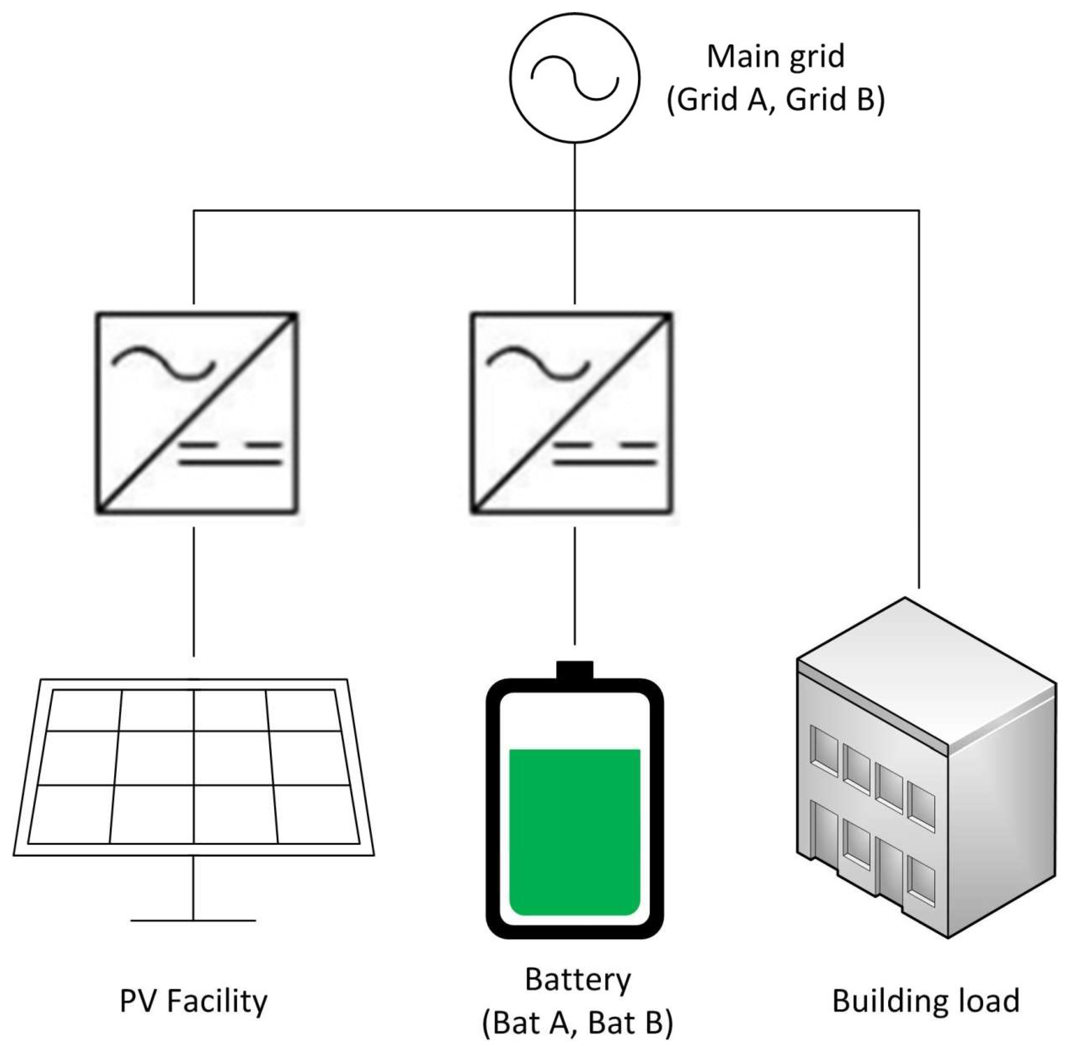
The proposed method is designed to optimally use an energy storage system on a microgrid with a load and generation system connected to the distribution grid. For the rest of this document, a battery and a PV facility will be assumed to play the energy storage and generation systems, as those were employed during the tests. Figure 1 shows the model of the microgrid.
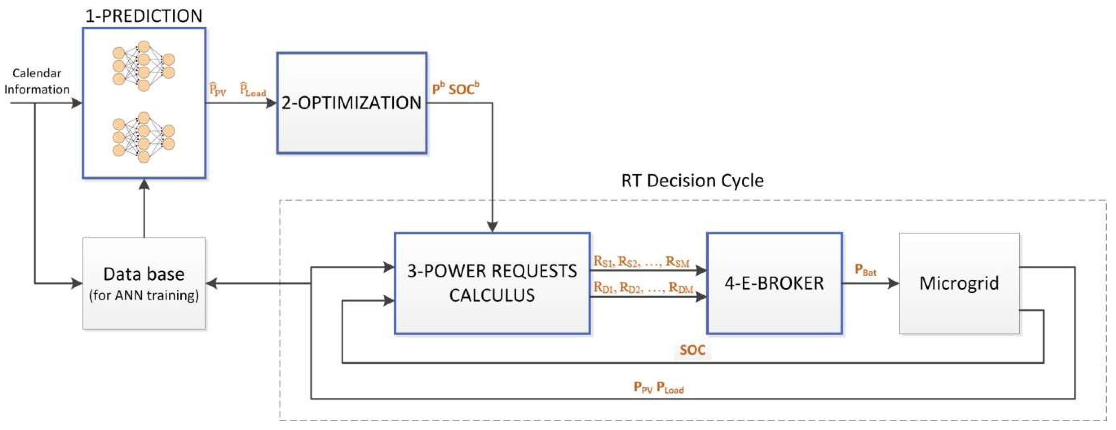
The method comprises four key operations: a prediction, an optimization, several power requests definitions, and an auction. The prediction and the optimization are applied once a day, while the power requests and the auction are executed continuously as a real time (RT) decision cycle.
The power requests (R), which are made on behalf of the devices of the microgrid, represent how much power each device is capable provide as a supplier (RS) or absorb as a demander (RD). For example, a power request is associated with the PV facility and indicates how much power it can provide. Similarly, a power request is associated with the load indicating how much power it will consume. Power requests are made for all devices, including the main grid. The auction algorithm, or E-Broker, then calculates how much power must be transferred between the different devices according to these power requests and a priority system. The power requests corresponding to the battery and main grid are split, as if they were respectively modeled as two batteries (Bat A and Bat B) and two main grids (Grid A and Grid B). The E-Broker treats these power requests with different priorities, so the whole system will behave differently depending on how these power request divisions are made. These power requests divisions (between Grid A and B, and between Bat A and B) depend on two variables: Pb and SOCb.
The values of Pb and SOCb are obtained through the aforementioned optimization process. At the beginning of each day, a heuristic optimization function chooses the best evolution of these variables along the day to reduce the expected electricity bill as much as possible. To do so, the optimization process considers the initial state of the battery and the electricity prices. Additionally, since the load consumption and the PV generation cannot be controlled (except for generation curtailment), the optimization process considers a prediction for the power consumed or generated by these devices. This prediction is made just before the optimization process.
Figure 2 shows the inputs and outputs of each operation. These operations are further described below in its own subsection. The whole method has been programed in Python.
2.1.1. Prediction
As previously stated, the optimization process needs some prediction of the uncontrolled devices power: the load and the PV facility. The more accurate the prediction is, the more reliable the optimization will be. Nevertheless, the strategy employed to obtain this prediction is not a fundamental part of the general method. The procedure described here was used to obtain the results of Section 3; other prediction methods, like the future work mentioned in Section 4, would work as well.
Predictions of loads and generation are obtained at the beginning of each day using artificial neural networks (ANNs). These predictions occur at midnight and consider only calendar information: the month, the day of the week, and the type of day (working day or holiday). For the tests, the load corresponded to a laboratory building in the University of Seville. Since the usage of the building follows a schedule, the calendar information is enough to obtain good predictions. The PV facility is harder to predict as it depends on the weather. However, calendar information is good enough for average and cloudless days. In the future, more weather-related inputs will be included to cover the possibility of cloudy days.
The ANNs used for the tests have been programmed in Python using the Keras package for Deep Learning, which runs on top of Theano (see [28] for more information about the Keras package). The activation function of the ANNs uses the rectifier activation function or Rectified Linear Unit (ReLU). The mean square error is minimized in the compilation. The “adam” efficient gradient descent algorithm is also used for its high efficiency. The number of iterations run for the training process (epochs) is 200. The number of evaluated instances before updating the weights (batch size) is 2.
Two ANNs are used for the predictions: one for the PV () facility and another for the load (). The ANNs are structured in three layers of 70, 50, and 96 neurons; with 3 inputs for calendar information and 96 outputs for the predicted quarter-hourly power values. These output power values are assumed to be the average power produced or consumed by the corresponding device during a 15-min window. All ANNs have been trained with 1-year historical data, using 70% of the data for training and the remaining 30% for evaluation.
2.1.2. Optimization
After the prediction, an optimization process is run to find the best suited evolution for Pb and SOCb according to the prediction. These values will later serve as boundaries to determine the behavior of the grid and the battery regarding the power auction.
The selected algorithm for this optimization is the PSO, which is typical and efficient for this type of problem according to [15]. If the priorities of the E-Broker auction, which only consider relative order, needed to be optimized, then the genetic algorithm (GA) would be suitable. This is so because the GA works better with discrete variables. However, the proposed priorities are already optimal for this microgrid. Since PSO works better than GA for continuous variables, PSO is preferred.
The PSO method is imported from library pyswarm for Python. The swarm size is specified to be 2000 particles. The stop conditions are also specified: the maximum number of iterations is 200, the minimum step of the particles is 0.0001 and the minimum change of the objective function is 0.0001€/month. This way, once iterations have no real impact on the yearly electricity cost, the method stops. The default values are used for the remaining parameters, which define the movement of the particles.
Aside from the upper and lower limits of Pb and SOCb, no constraints need to be imposed. This is so because the power requests and the auction algorithm always command the battery to exchange a feasible amount of power with another device capable to do so. The absence of constraints ensures a connected and convex space of candidate solutions, which simplifies the movement of the particles in the PSO.
The optimization variables are the necessary parameters to parametrize Pb and SOCb. Pb is a boundary for the grid power that triggers a different behavior of the grid regarding the power requests. The grid power requests will have a higher priority as long as the grid power is below Pb. Tests indicate that the best evolution for Pb is to remain constant, so it can be defined with only one optimization variable xp. Pb is chosen to be proportional to the contracted power Pcont and to the optimization variable xp, which is bounded between 0 and 1. Although this is not expected, Pb is allowed to be greater than the contracted power.
Pb = 2·Pcont·xp
Similar to Pb, SOCb is a boundary for the battery state of charge (SOC) that triggers different power requests. Several piecewise polynomial interpolations have been tested to parametrize the best behavior of SOCb with the PSO selecting both the time and the SOCb value for each point. Best results have been obtained with a lineal interpolation between 13 points for each day. The first is at midnight and its value corresponds to the actual SOC of the battery at the time of the optimization. The last point is 24 h later. Both coordinates of the remaining points, as well as the value of SOCb for the last point, are optimization variables for the PSO algorithm. Variables that define the time coordinate of these points are bounded between 0 and 1, which correspond to the beginning and the end of the day respectively. Variables that define the SOCb coordinates are bounded between 0.1 and 0.95, which correspond to 10% and 95% of the battery allowed SOC range.
The objective function is the total grid electricity cost for a month with 30 equal days according to Spanish tariff 3.0A. This tariff considers the time of use (TOU) for energy and power by dividing the day into three periods with different prices. On each period, the energy cost depends on the total amount of energy provided by the grid during each period while the power cost depends on the highest power peak PPeak of each period. Details of these costs can be consulted on [29]. At the moment of writing this paper, the Spanish legislation does not allow consumers to sell electricity, so this situation is not considered. Nevertheless, it is possible to consider this case by adding power requests on behalf of the grid as a demander.
To evaluate the objective function, the PSO simulates the actions of the RT decision cycle (the Power requests calculus and the E-Broker auction algorithm) according to the values of Pb and SOCb. Thus, each evaluation of the objective function requires simulating a day divided into 96 equal intervals of 15 min. Please note that the sample time of the actual RT decision cycle is 5 s. The 15-min sample time is just a simplification to be able to run so many simulations. On all these simulations, the load and the PV facility are assumed to consume or generate the previously predicted average power for each interval.
Each simulation obtains the total energy cost CETotal as
where CE k and PGrid k are the energy cost and the power provided by the grid during interval k. The total power cost CPTotal is calculated as
where CP k and PPeak k are the power cost and the maximum peak registered for period k, and function f(PPeak k) is defined according to the Spanish legislation.
Pcont is the contracted power, which can be changed once a year if the user so desires, but for the optimization it is considered to be a known constant. The value of the objective function FObj is calculated by adding the total energy cost of 30 equal days and the total power cost for the month:
FObj = CPTotal + 30·CETotal
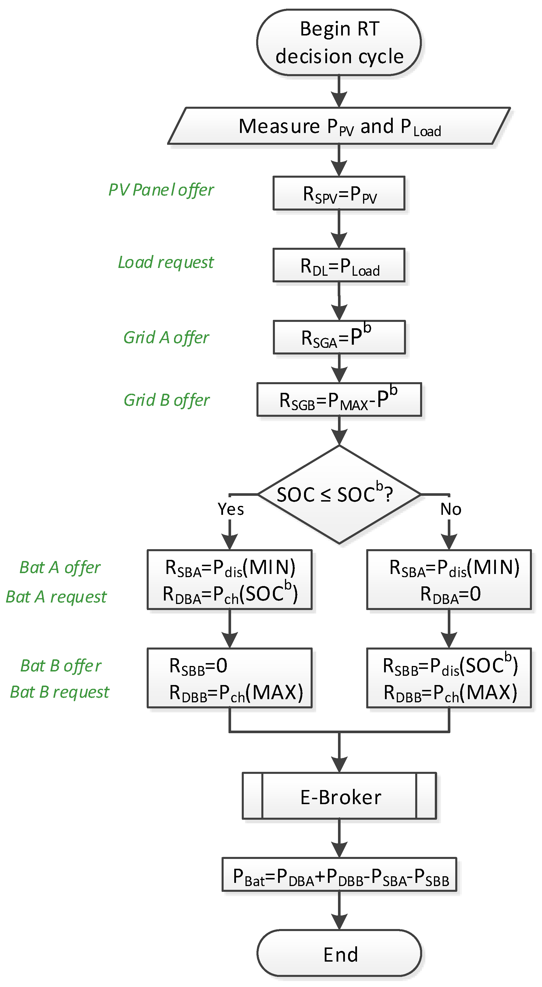
2.1.3. Power Requests Calculus
Power requests are calculated on real time according to the measures and optimization values. Afterwards, they are sent to the E-Broker auction algorithm, where they function similar to power bids. Several power requests may be associated with the same device. Figure 3 summarizes how the values of power requests are calculated for each device.
The actual power generated by the PV facility PPV and the power consumed by the load PLoad are measured. A power request is made on behalf of each one (RSPV and RDL) to provide or receive the same power they are respectively generating or consuming. These two devices are not actually requesting permission to produce or consume such power; they will do it anyway as they are not controlled. Thus, to ensure the E-Broker auction algorithm always serves these requests, they will be given the highest priority.
The power grid is associated to two power requests: RSGA and RSGB. This can be understood as dividing the grid into two different suppliers (Grid A and Grid B) that, together, can provide up to the grid maximum power PMAX. The value of RSGA is Pb, the optimal power limit of the grid. The rest of the power the grid can provide is assigned to RSGB. RSGA will later have a higher priority than RSGB, so an attempt will be made to limit the grid power to Pb. Nevertheless, thanks to RSGB, it is possible to go beyond this limit, if absolutely necessary.
The battery is also symbolically divided into two sections: Bat A, whose charge capacity is only up to SOCb, and Bat B, with the rest of the capacity. Each battery section will make a power request to provide power (RSBA and RSBB) and a power request to absorb power (RDBA and RDBB). These power requests depend on the actual SOC of the whole battery, which is measured by the battery management system.
When the actual SOC is lower than SOCb, battery section A will request to absorb the necessary power Pch(SOCb) to reach SOCb as quickly as possible within the limits of the battery power capabilities. If it is possible to reach SOCb in just one iteration of the RT decision cycle, then Pch(SOCb) is the necessary power to do so; otherwise, Pch(SOCb) is the battery nominal charge power. Battery section B will not request to provide any power while SOC is below SOCb.
On the other hand, when the actual SOC is higher than SOCb, battery section B will request to provide the necessary power Pdis(SOCb) to discharge back to SOCb as quickly as possible within the battery capabilities. Again, if it is possible to reach SOCb in one iteration, Pdis(SOCb) is the necessary power to do so; otherwise, it is the battery nominal discharge power. Battery section A will not request to charge any power.
Either way, with any remaining discharge power, battery section A will request to discharge to the battery minimum charge Pdis(MIN). Similarly, battery section B will request to charge to the battery maximum charge with any available charge power left Pch(MAX).
Battery section A has a higher priority to charge and battery B has a higher priority to discharge. Hence, the battery SOC will tend to follow SOCb when possible. Nevertheless, it is still possible to deviate from SOCb, since the battery corresponding section always requests to charge or discharge to its limits.
Once all power requests have been calculated, the E-Broker auction algorithm is executed.
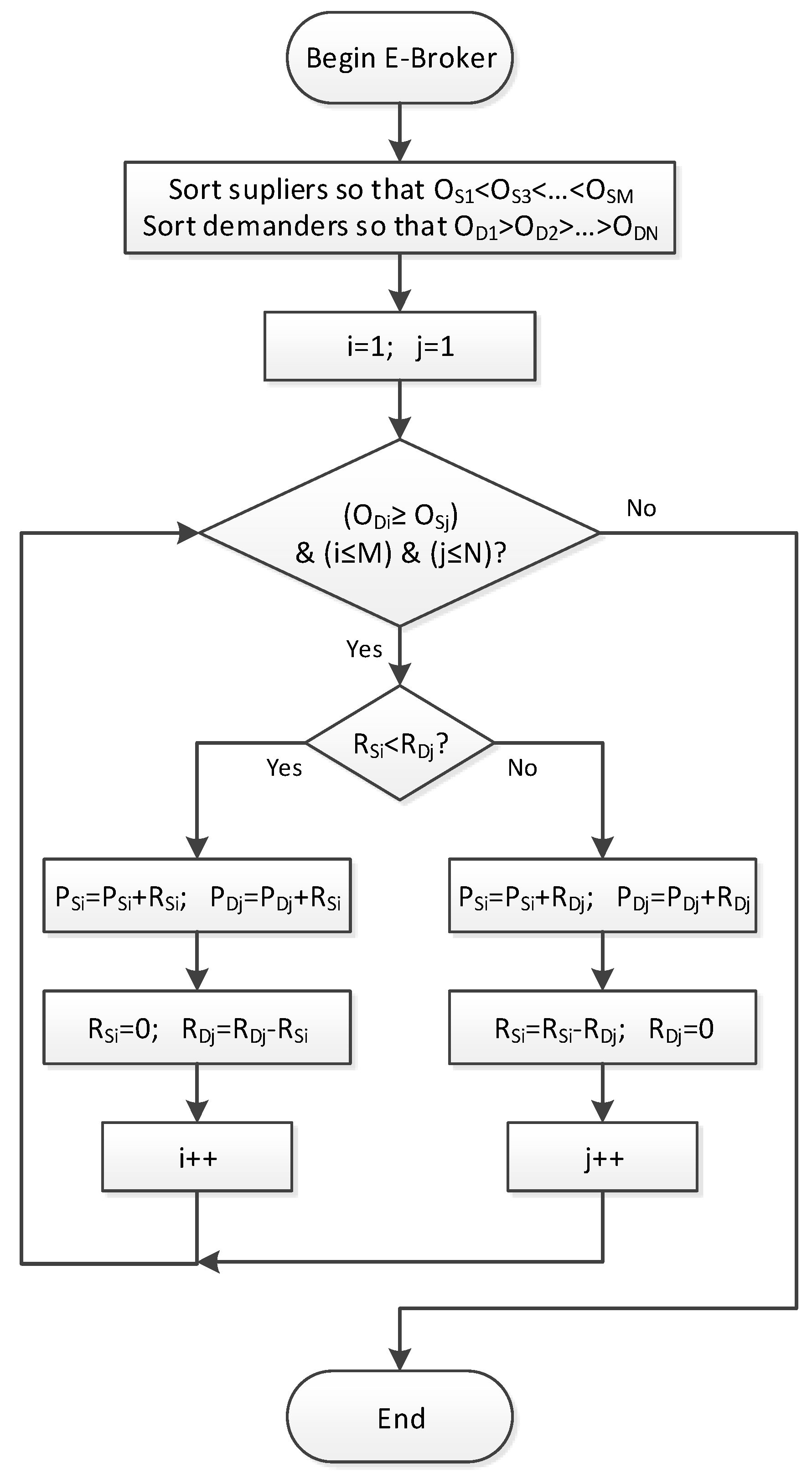
2.1.4. E-Broker Auction Algorithm
The algorithm used for the auction is a version of the one described in [3], where only the own priorities of the suppliers and the limit priorities of the demanders are used. It can be defined as a real time (RT) multi-agent system (MAS) that receives the power requests (R) made by M suppliers and N demanders and decides whether to address them or not according to the suppliers’ priority values (OSi) and demanders’ priority values (ODj).
Any prosumer (such as a battery) is considered as both a supplier and a demander. In addition, as previously explained, optimized elements such as the battery and the network can be included in the auction as several participants each: Bat A, Bat B, Grid A, and Grid B.
Suppliers and demanders are sorted according to their priority values. Higher priorities are represented with greater priority values for demanders and with smaller values for suppliers. In addition, for an exchange between supplier i and demander j to occur, the priority value of the demander (ODj) must be greater than or equal to that of the suppliers (OSi). This is similar to a market auction where priority values act as prices. Table 1 shows the sorted suppliers and demanders, their priority values and whether a combination is allowed (A) or forbidden (X).
Devices are checked in priority order and each demander is searched for a supplier with equal or lower priority that has power available to feed it. This way, the algorithm calculates the power each supplier must provide PS1…PSM and each demander must receive PD1…PDN, having a balance between the total power delivered and received. Figure 4 summarizes the E-Broker Auction Algorithm.
Since the power requests for the PV facility and the loads were based on the actual power of these devices, and the distribution grid is not controlled from the microgrid, only the battery power needs to be applied. To do so, the inverter connected to the battery is commanded to charge (or discharge) the battery at a certain power rate. The net power the battery must absorb is PBat, which is calculated from the power values selected by the E-Broker algorithm as shown in Figure 3.
A detailed example is provided for better clarity. Table 2 shows the power requests (R), as well as the final powers (P) each device must provide or receive.
For this example, the battery can charge or discharge at 5 kW and at the point of the shown execution of the RT cycle SOC is lower than SOCb. Therefore, Bat A makes a request as a demander to get to SOCb: 3 kW, which is enough to get to SOCb by the next cycle. Bat B requests to keep charging with the remaining charge power (2 kW) in case there is an excess of PV power. Bat A also requests to discharge at up to its maximum rate (5 kW) if needed.
The power request of Grid A is given by Pb which, in this example, is 8.5 kW. Due its priority, the power of Grid B will only be used if the power required by the load is greater than the sum of the powers of the PV facility, Grid A, and the battery. This will help preventing grid power peaks greater than Pb.
The E-Broker algorithm starts by checking the first demander (the Load) and the first supplier (the PV facility). It verifies that the priority of the demander is greater than the priority of the supplier, so the exchange is allowed. The load request is greater than the PV facility request, so all the power of the PV facility is assigned to the load.
The PV facility has exchanged all its power, but the Loads still request to receive 8 kW more. The E-Broker algorithm searches for the next supplier with a power request greater than 0: Grid A. It is verified that the priority of the loads is still greater than that of Grid A. Thus, the remaining power that was missing from the load is exchanged, 8 kW, leaving Grid A with 0.5 kW available to assign.
The algorithm confirmed that the priority of the next demander (Bat A) is greater than that of Grid A. The exchange is possible, so the remaining 0.5 kW of Grid A are assigned to Bat A. The remaining 2.5 kW of Bat A must stay unassigned since all other suppliers have greater priority values. There are no other demanders whose priority is greater than those of the remaining suppliers, so no more power can be assigned.
In the end, the PV facility provides 4 kW (as originally measured), the load consumes 12 kW (as measured), the battery is commanded to charge at 0.5 kW and the grid provides the difference: 8.5 kW. Please note that even though the E-Broker algorithm considers power transferring in pairs of devices (a supplier and a demander) the actual route of the power may be different. For example, the 0.5 kW used to charge the battery may actually be coming from the PV facility. The E-Broker only decides how much each device exchanges, not which device it is exchanged with.
2.2. Implementation and Test Description
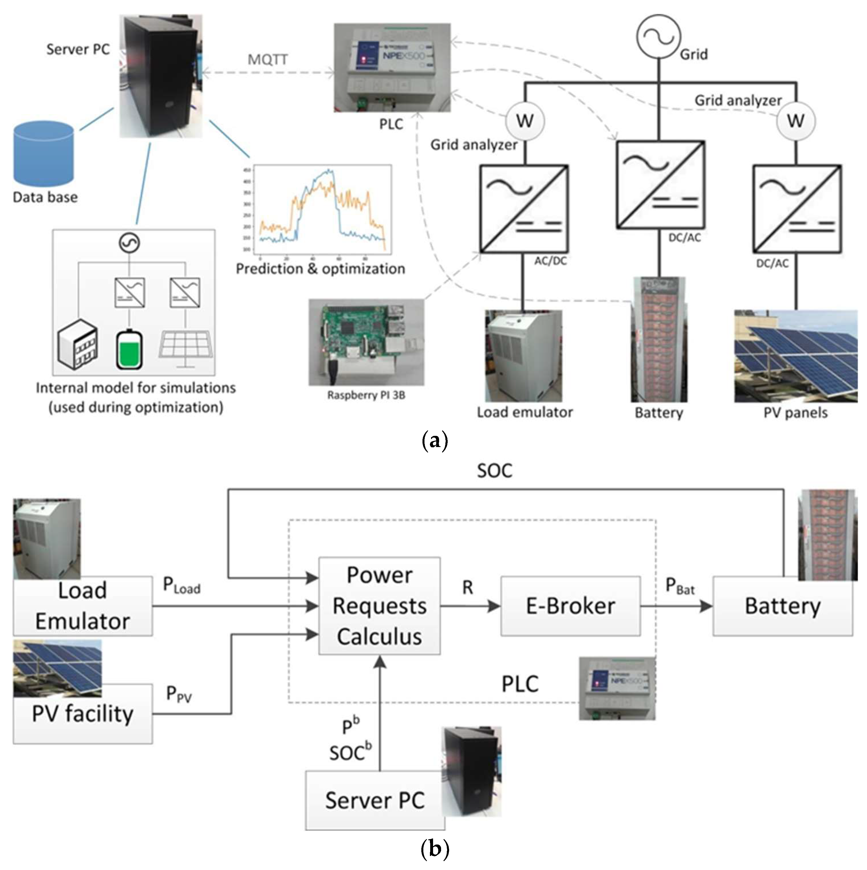
A test bench has been built to validate the proposed method, as shown in Figure 5. Here, a 20-kW PV system and a 10-kWh-energy and 5-kW-power battery are employed. The load is emulated using a revertible power source and an inverter controlled by a raspberry pi (model 3B). This load emulation system is programed to consume power according to historic data from previous days.
The proposed method is distributed among a programmable logic controller (PLC) and a personal computer (PC) acting as a server, which communicate with one another using the message queue telemetry transport (MQTT) protocol.
As shown in Figure 6, the server PC runs the aforementioned prediction and optimization at the beginning of each day. After each optimization, the PC server sends to the PLC the necessary parameters so that the latter can reconstruct Pb and SOCb through linear interpolation.
Using this information, the PLC receives the measured power values of the load and PV systems, runs the RT decision cycle shown in Figure 3 and Figure 4, and commands the battery inverter to charge or discharge the battery accordingly. This RT decision cycle is executed every 5 s.
Every 15 min, the PLC reports the average PV power production, load consumption, and battery SOC for that time period. This information is stored in a data base to train the ANNs, as well as to evaluate the results of the proposed method.
The tests have been performed considering days independently. Since the power cost can only be evaluated for periods of at least one month, the grid electricity bill has been calculated considering 30 equal days. The prices used and their corresponding time periods are shown in Table 3. The objective function has been calculated considering the Contracted Power is 10 kW.
Among the referenced publications for optimal scheduling, [17,22] are the newest ones. The method from [22] aims for the same purpose and considers some real-time control. The method from [17], on the other hand, intends to control a whole distribution grid and would be harder to adapt. Thus, the proposed method is compared to [22], which can be considered the state of the art. Since the method from [22] did not originally consider PV generation, an additional adjustment has been made to it: whenever the PV generation is greater than the load power, the battery will attempt to absorb the power excess in the same way it would attempt to prevent power peaks. This can be understood as the battery avoiding a negative power peak. This adjustment always produces a better result as otherwise this extra power would be unused. The simulation is run for the same day, with the same power values for the PV generation and load consumption, and the method from [22] is provided the same prediction as the proposed method had at the beginning of the day, so that they can be compared under the same conditions.
3. Results
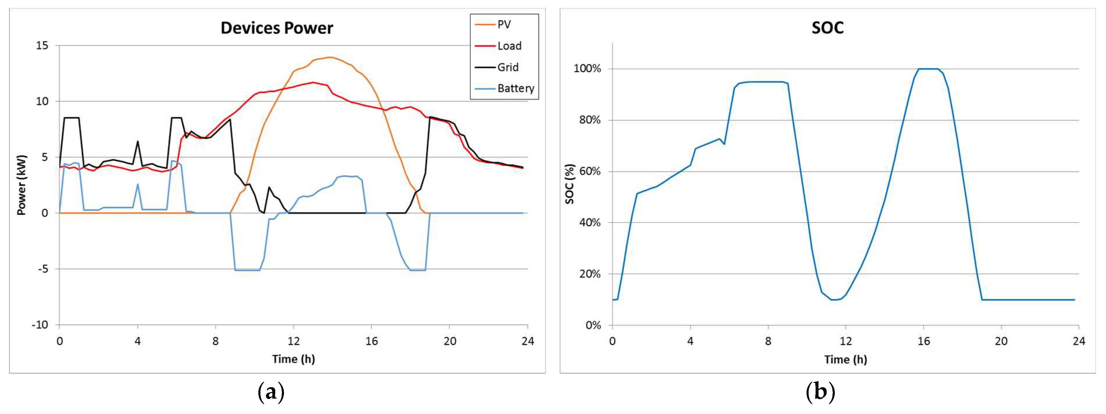
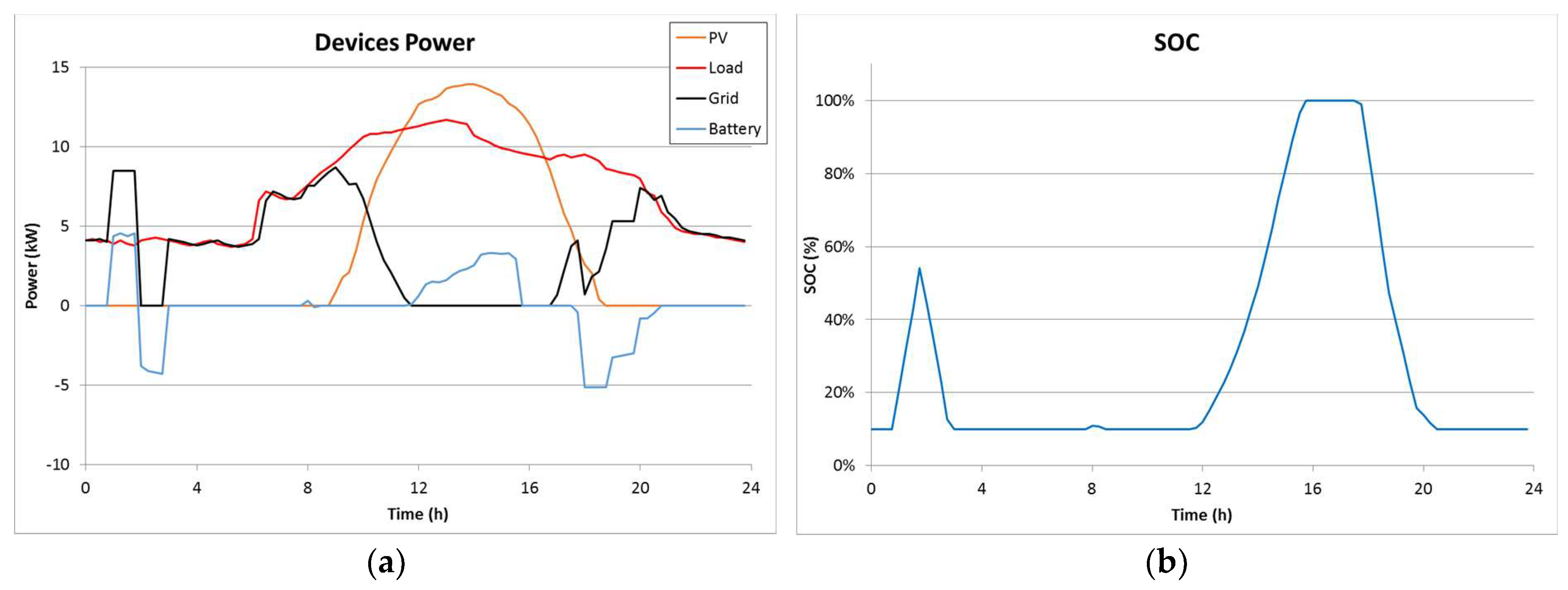
Figure 7 shows the results of a real test performed on 26 September 2018 in the Laboratory of Electronic Engineering Department of the University of Seville.
The battery is used mainly for energy shifting. It first charges during the cheapest period, before dawn, and uses that energy at the beginning of the second period. This, along with the PV power keeps the grid power to a minimum. Afterwards, when the PV generation exceeds the load power, the battery absorbs the difference, which is used in the evening, during the most expensive period. In addition, the grid power never exceeds the 85% of the contracted power, which keeps the power cost at the minimum.
It is worth noting that the battery power follows the PV generation peaks near midday, maintaining the grid power low and stable. This is possible because the RT decision cycle acts according to the measured load and PV power. If an optimal power plan obtained from imperfect predictions had been applied on an open loop, the grid power would have oscillated around zero. Sometimes, power would have flown to the grid (which is not allowed). This exemplifies why the RT decision cycle is important.
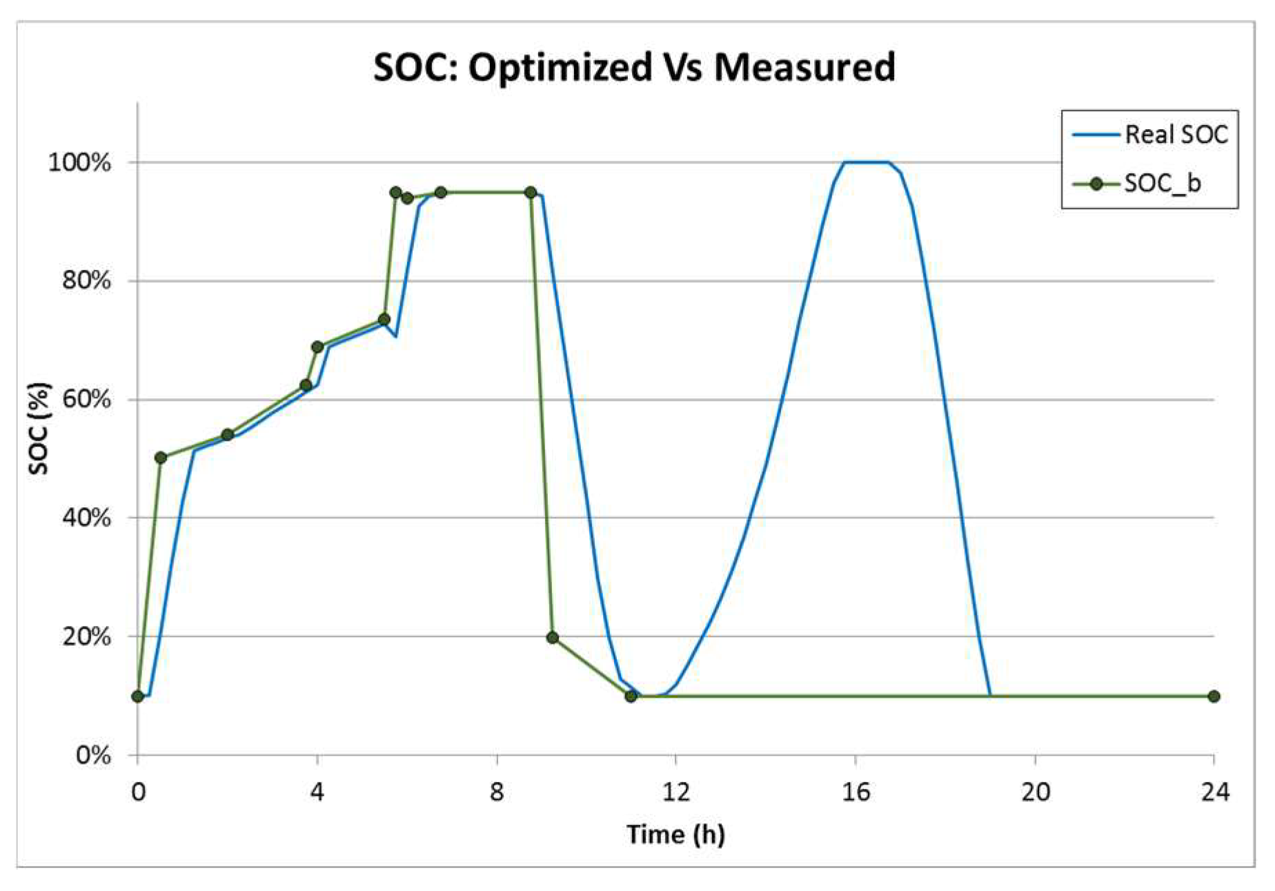
Figure 8 shows the results of the optimization for SOCb and compares them with the evolution of the actual SOC.
Two important details should be appreciated in this figure. The first one is how the battery SOC tends to follow SOCb during the first half of the day only. As previously explained, the priorities are chosen so that SOC follows SOCb when possible, so the first half of the day demonstrates that the optimization has an impact on the trend of the SOC. However, after midday, there is a surplus of PV generation, which the battery must absorb due to the specified priorities. Again, the RT decision cycle overruns the optimization plan so that the PV power surplus is not wasted.
The second detail to note is how all the points that describe SOCb are before midday. As explained, the optimization process selects both coordinates of these points. When the predictions are considered, the optimization finds no benefit in adding points to the second half of the day. After all, according to the predictions, the battery behavior during the evening will not depend on SOCb, but on the PV power surplus. Consequently, the PSO uses all the points to produce and parametrize the optimal trend of SOCb during the morning.
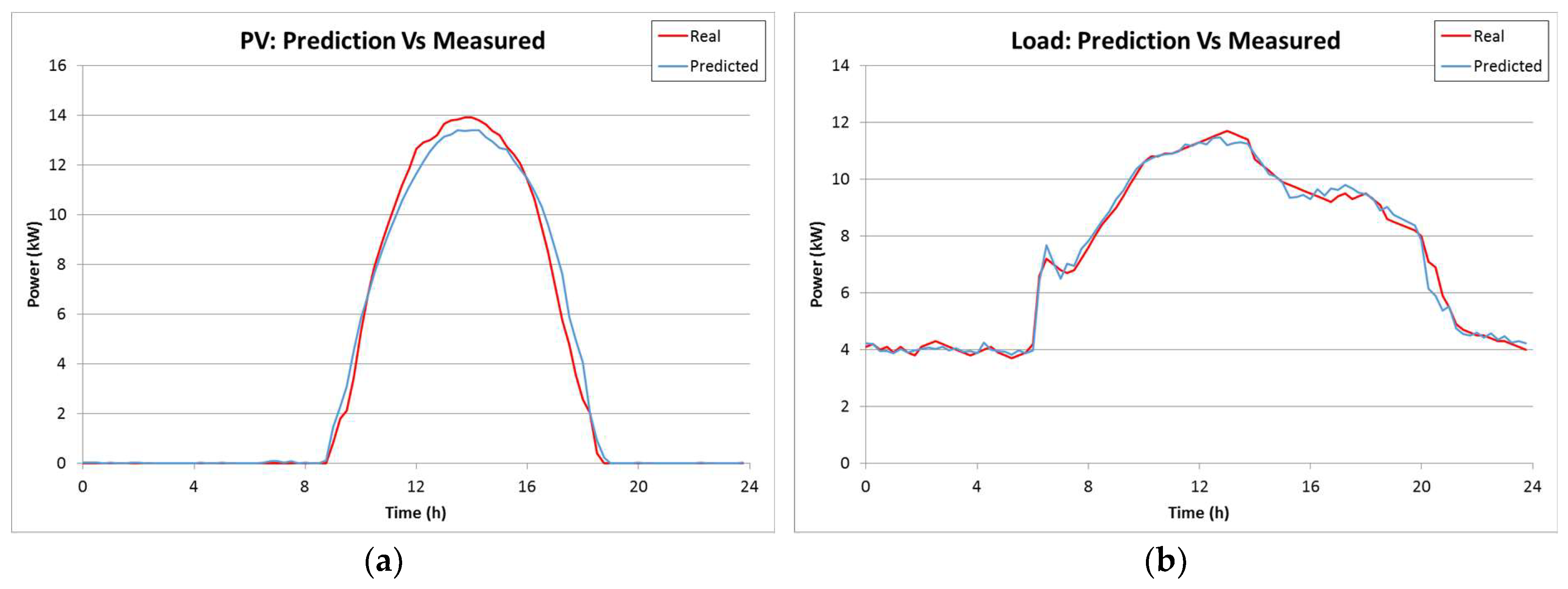
Figure 9 shows the predicted and real power values for the PV facility and load respectively. As previously stated, these predictions were obtained using artificial neural networks whose input solely consists of calendar information.
It is important to note that the predictions are similar to the reality, but not equal. The fact that the general shape of each curve is correct is enough to let the PSO find the optimal plan for SOCb. The small differences will be corrected during by the RT decision cycle. Nevertheless, the predictions were quite accurate the day of the test.
Although the power peaks are still prevented and the battery power follows the PV generation, the energy shifting is much poorer. The battery even charges and discharges on the same tariff period with no real benefit (and with the consequent losses due to its efficiency). Since the battery is empty when the load power rises, there is an unavoidable peak which slightly increases the power cost. The filling of the battery after midday occurs due to the prevention of a (negative) power peak on the grid, and would also have occurred regardless of the optimization result.
In general, the optimization in this method is not as good as in the presented one. It might have done better with a higher number of particles or longer time. Since both methods used the same parameters to define the PSO, it can be concluded that the proposed method converges better. Considering the proposed method only requires one optimization at the beginning of the day, while method from [22] requires an optimization each hour, this is an important advantage.
Table 4 shows the values of the electrical bill for both methods so that they can be compared with ease. Additionally, the case where no battery is present has been added to the table so that both methods can be compared with the absence of any method. As shown, the proposed method saves 4.41% over the state-of-the-art method, and 8.12% over the original cost. It is also worth noting that the method from [22] cannot save any power cost with peak shaving in this situation.
4. Discussion
The most evident result is the fact that the proposed method can reduce the grid power and energy cost more than the previous method. The strategy of the proposed method is shown to be more consistent, while the successive optimizations of the method from Ref. [22]’s alternative tend to produce an erratic behavior, with the battery charging and discharging on the same price period for no apparent reason. This occurs because the optimization problem is badly conditioned. The grid peak limit, which is recalculated on every hourly optimization, conflicts with the remaining optimization variables. All variables represent power (whether from the battery or from the grid) and the RT control applies only the limiting one. Consequently, some of the variables have no impact on the objective function while others compete with one another to produce any impact. In contrast, the method proposed in the present paper is capable of reallocating the points that define SOCb, so that all variables have some impact on the objective function. This helps particles of the PSO find a unique solution rather than iterating along a family of very similar solutions.
In addition, the PV generation and load behavior allows for several quasi optimal alternatives and the hourly optimization keeps changing the strategy constantly. While the optimal battery power plan (obtained in [22]) is heavily dependent on the PV generation and load consumption, the optimal SOC boundary (obtained according to the proposed method) is much more robust and stable. This is so because the SOC, being the integral of the battery power, acts as a low pass filter. Methods that optimize the power of the battery (instead of the SOC) will find similar difficulties, particularly if they must optimize periodically to reassess the plan.
It is possible to add constraints to the PSO that would prevent the battery from discharging and charging in the same tariff period. For example, the total number of battery power changing signs could be limited. However, adding many constraints produces non-convex search spaces for the particles, which makes it harder to find the solution. An excess of constraints could even isolated particles from one another if the search space becomes non-connected. The proposed method does not require any constraint except for the limits of each variable (typically normalized between 0 and 1). This helps the convergence speed.
The lack of constraints is possible due to the way the power requests are calculated. Regardless of the optimization results, no device in the microgrid is ever forced to produce or absorb an impossible amount of power. For example, if for any reason the load consumption was cut unexpectedly, the battery would not provide more power. In fact, even if the prediction or the optimization is badly performed, the battery will not be commanded to provide or exchange power if there is no other device to exchange it with.
Optimizing only the boundaries of the battery behavior, as proposed is another advantage as it allows the battery to absorb or provide unexpected power to prevent peaks or avoid power losses. The battery can act as a dynamic reserve both for peak shaving and energy shifting. This, combined with the priority system from the E-Broker Auction Algorithm is responsible for the robustness of the method. This is important especially because the predictions only consider calendar information (and not the weather forecast) and thus may not be perfectly accurate. This proves that the proposed method can cope with some unpredicted situations.
Nevertheless, since the predictions must be accurate enough for the PSO to find a general plan for the SOCb, future versions of the proposed method will consider weather forecast information. This information is expected to include humidity, clarity of the sky, and temperature of every hour. Currently, the proposed method does not require hourly optimizations, so the strategy is maintained coherent for longer periods of time and computational costs are lowered. However, authors consider the possibility of optimize again midway through the day if predictions are found to deviate too much from measured power values. This has not been implemented yet but will be tried in future versions.
Another aspect of the proposed method that shares with the method from [22] is the fact that no division needs to be imposed on the battery to distinguish peak shaving from energy shifting. The proposed method optimizes the appropriate variables (SOCb for energy shifting and Pb for peak shaving) so that no capacity needs to be wasted.
In the future, other applications for the proposed method are expected, such as demand control by price or frequency response. Although this will require predicting and optimizing additional magnitudes, the general concept of the method will remain intact: long-term optimization and real time decision making. These new applications, just like the presented one, will save storage costs because the method will provide the best possible use for the batteries. As for the exposed application, since the power and energy cost reflects how much power the main grid is moving at any given hour, reducing the energy bill helps decongesting the grid during the peak hours.
Finally, an important aspect of the proposed method is the fact that the E-Broker auction algorithm is based on a method originally designed for microgrids operation with distributed resources. Consequently, the proposed method is an evolutionary step towards the smart grids and distributed paradigm that can be applied in the present time. This serves as an intermediate state between the current energy system situation and the utopic approaches from other publications (see [1,2,3,4] for examples). We hope the proposed method helps us reach a new and better future.
5. Patents
International patent application WO2015/113637A1 results from part of the work reported in this manuscript. The described E-Broker auction algorithm is based on a simplification of the method disclosed in the patent. Please note that the rest of the proposed method is original and helps improving the performance of the patented method.
Author Contributions
Conceptualization, L.G., E.G., and A.A.; Software and data curation, J.M.N.; Investigation, L.G., J.M.N., and A.A.; Resources, E.G. and J.M.C.; Methodology, Validation and formal analysis, all authors; Writing—original draft preparation, L.G. and J.M.N.; Writing—review and editing, E.G., J.M.C., and A.A.; Visualization, all authors.; Supervision, E.G., J.M.C., and A.A.; Project administration and funding acquisition, E.G. and J.M.C.
Funding
This research was funded partially by the European Commission for the Seventh Framework Programme under grant agreement ID 771066 and partially by the Spanish Ministry of Economy and Competitiveness under, grants ENE2016-80025-R and RTC-2016-5634-3.
Acknowledgments
The starting point of this research were the results of the projects Pollux and IoE, which were funded by the European Commission for the Seventh Framework Programme under grant agreement IDs 100205 and 269374. Green Power Technologies SL is also acknowledged for supporting the experiments with previous demonstrators.
Conflicts of Interest
The authors declare no conflict of interest. The funders had no role in the design of the study; in the collection, analyses, or interpretation of data; in the writing of the manuscript, or in the decision to publish the results.
References
- Bliek, F.; Noort, A.; Roossien, B.; Kamphuis, R.; Wit, J.; Velde, J.; Eijgelaar, M. PowerMatching City, a living lab smart grid demonstration. In Proceedings of the 2010 IEEE PES Innovative Smart Grid Technologies Conference Europe (ISGT Europe), Gothenberg, Sweden, 11–13 October 2010. [Google Scholar] [CrossRef]
- Kamphuis, I.G.; Eijgelaar, B.R.M.; de Heer, H.; van de Velde, J.; van den Noort, A. Real-time trade dispatch of a commercial VPP with residential customers in the PowerMatching City SmartGrid living lab. In Proceedings of the 22nd International Conference and Exhibition on Electricity Distribution, Stockholm, Sweden, 10–13 June 2013. [Google Scholar] [CrossRef]
- Martín, P.; Galván, L.; Galván, E.; Carrasco, J.M. System and Method for the Distributed Control and Management of a Microgrid. Patent No. WO2015113637, 6 August 2015. [Google Scholar]
- Flikkema, P.G. A Multi-Round Double Auction Mechanism for Local Energy Grids with Distributed and Centralized Resources. In Proceedings of the 2016 IEEE 25th International Symposium on Industrial Electronics (ISIE), Santa Clara, CA, USA, 8–10 June 2016. [Google Scholar]
- Raju, L.; Rajkumar, I.; Appaswamy, K. Integrated Energy Management of Micro-Grid using Multi Agent System. In Proceedings of the 2016 International Conference on Emerging Trends in Engineering, Technology and Science (ICETETS), Pudukkottai, India, 24–26 February 2016. [Google Scholar] [CrossRef]
- Nunna, H.K. An Agent based Energy Market Model for Microgrids with Distributed Energy Storage Systems. In Proceedings of the 2016 IEEE International Conference on Power Electronics, Drives and Energy Systems (PEDES), Trivandrum, India, 14–17 December 2016. [Google Scholar] [CrossRef]
- Mohsenian-Rad, H. Optimal Bidding, Scheduling, and Deployment of Battery Systems in California Day-Ahead Energy Market. IEEE Trans. Power Syst. 2016, 31, 442–453. [Google Scholar] [CrossRef]
- de la Nieta, A.A.S.; Tavares, T.A.M.; Martins, R.F.M.; Matias, J.C.O.; Catalão, J.P.S.; Contreras, J. Optimal Generic Energy Storage System Offering in Day-Ahead Electricity Markets. In Proceedings of the 2015 IEEE Eindhoven PowerTech, Eindhoven, The Netherlands, 29 June–2 July 2015. [Google Scholar] [CrossRef]
- Zhang, Z.; Wang, J.; Wang, X. An improved charging/discharging strategy of lithium batteries considering depreciation cost in day-ahead microgrid scheduling. Energy Convers. Manag. 2015, 105, 675–684. [Google Scholar] [CrossRef]
- Wang, R.; Wang, P.; Xiao, G. A robust optimization approach for energy generation scheduling in microgrids. Energy Convers. Manag. 2015, 106, 597–607. [Google Scholar] [CrossRef]
- Mohamed, F.A.; Koivo, H.N. Multiobjective optimization using Mesh Adaptive Direct Search for power dispatch problem of microgrid. Int. J. Electr. Power Energy Syst. 2012, 42, 728–735. [Google Scholar] [CrossRef]
- Hosseinnezhad, V.; Rafiee, M.; Ahmadian, M.; Siano, P. Optimal day-ahead operational planning of microgrids. Energy Convers. Manag. 2016, 126, 142–157. [Google Scholar] [CrossRef]
- Morais, H.; Kádár, P.; Faria, P.; Vale, Z.A.; Khodr, H.M. Optimal scheduling of a renewable micro-grid in an isolated load area using mixed-integer linear programming. Renew. Energy 2010, 35, 151–156. [Google Scholar] [CrossRef] [Green Version]
- Sousa, T.; Morais, H.; Vale, Z.; Faria, P.; Soares, J. Intelligent energy resource management considering vehicle-to-grid: A simulated annealing approach. IEEE Trans. Smart Grid 2012, 3, 535–542. [Google Scholar] [CrossRef]
- Yang, Y.; Zhang, W.; Jiang, J.; Huang, M.; Niu, L. Optimal Scheduling of a Battery Energy Storage System with Electric Vehicles’ Auxiliary for a Distribution Network with Renewable Energy Integration. Energies 2015, 8, 10718–10735. [Google Scholar] [CrossRef] [Green Version]
- Faria, P.; Soares, J.; Vale, Z.; Morais, H.; Sousa, T. Modified Particle Swarm Optimization Applied to Integrated Demand Response and DG Resources Scheduling. IEEE Trans. Smart Grid 2013, 4, 606–616. [Google Scholar] [CrossRef] [Green Version]
- Wang, Z.; Negash, A.; Kirschen, D.S. Optimal scheduling of energy storage under forecast uncertainties. IET Gener. Transm. Distrib. 2017, 11. [Google Scholar] [CrossRef]
- Yoon, Y.; Kim, Y.-H. Charge Scheduling of an Energy Storage System under Time-of-Use Pricing and a Demand Charge. Sci. World J. 2014, 2014, 937329. [Google Scholar] [CrossRef] [PubMed]
- Jia, X.; Li, X.; Yang, T.; Hui, D.; Qi, L. A Schedule Method of Battery Energy Storage System (BESS) to Track Day-Ahead Photovoltaic Output Power Schedule Based on Short-Term Photovoltaic Power Prediction. In Proceedings of the International Conference on Renewable Power Generation (RPG 2015), Beijing, China, 17–18 October 2015. [Google Scholar] [CrossRef]
- Lee, T.-Y. Operating Schedule of Battery Energy Storage System in a Time-of-Use Rate Industrial User with Wind Turbine Generators: A Multipass Iteration Particle Swarm Optimization Approach. IEEE Trans. Energy Convers. 2007, 22, 774–782. [Google Scholar] [CrossRef]
- Choi, Y.; Kim, H. Optimal Scheduling of Energy Storage System for Self-Sustainable Base Station Operation Considering Battery Wear-Out Cost. Energies 2016, 9, 462. [Google Scholar] [CrossRef]
- Kim, S.-K.; Kim, J.-Y.; Cho, K.-H.; Byeon, G. Optimal Operation Control for Multiple BESSs of a Large-Scale Customer Under Time-Based Pricing. IEEE Trans. Power Syst. 2018, 33, 803–816. [Google Scholar] [CrossRef]
- Celik, B.; Roche, R.; Bouquain, D.; Miraoui, A. Decentralized neighborhood energy management with coordinated smart home energy sharing. IEEE Trans. Smart Grid. 2017, 1–10. [Google Scholar] [CrossRef]
- Shah, S.; Khalid, R.; Zafar, A.; Hussain, S.M.; Rahim, H.; Javaid, N. An optimized priority enabled energy management system for smart homes. In Proceedings of the 2017 IEEE 31st International Conference on Advanced Information Networking and Applications (AINA), Taipei, Taiwan, 27–29 March 2017. [Google Scholar] [CrossRef]
- Li, V.; Logenthiran, W.T.; Woo, W.L. Intelligent multi-agent system for smart home energy management. In Proceedings of the 2015 IEEE Innovative Smart Grid Technologies-Asia (ISGT ASIA), Bangkok, Thailand, 3–6 November 2015; pp. 1–6. [Google Scholar] [CrossRef]
- Wang, L.; Wang, Z.; Yang, R. Intelligent multiagent control system for energy and comfort management in smart and sustainable buildings. IEEE Trans. Smart Grid 2012, 3, 605–617. [Google Scholar] [CrossRef]
- Hurtado, L.A.; Nguyen, P.H.; Kling, W.L. Smart grid and smart building interoperation using agent-based particle swarm optimization. Sustain. Energy Grids Netw. 2015, 2, 32–40. [Google Scholar] [CrossRef]
- Keras: The Python Deep Learning Library. Available online: https://keras.io/ (accessed on 17 January 2018).
- Spain Ministry of Economy. Real Decreto 1164/2001, de 26 de octubre, por el que se establecen tarifas de acceso a las redes de transporte y distribución de energía eléctrica; Boletín Oficial del Estado, BOE-A-2001-20850, No. 268. November 2001, pp. 40618–40629. Available online: https://www.boe.es/buscar/doc.php?id=BOE-A-2001-20850 (accessed on 17 January 2018).
Figure 1.
Microgrid model.

Figure 2.
Proposed method.

Figure 3.
Flow chart of the real time (RT) decision cycle. Power requests are detailed.

Figure 4.
E-Broker Auction Algorithm flow chart.

Figure 5.
Schemes of the test bench. (a) Devices and connections scheme. Black bold solid lines represent electrical connections, gray dashed lines represent communications and blue thin solid lines represent PC functions (b) Control scheme of the RT decision cycle.
Figure 5.
Schemes of the test bench. (a) Devices and connections scheme. Black bold solid lines represent electrical connections, gray dashed lines represent communications and blue thin solid lines represent PC functions (b) Control scheme of the RT decision cycle.

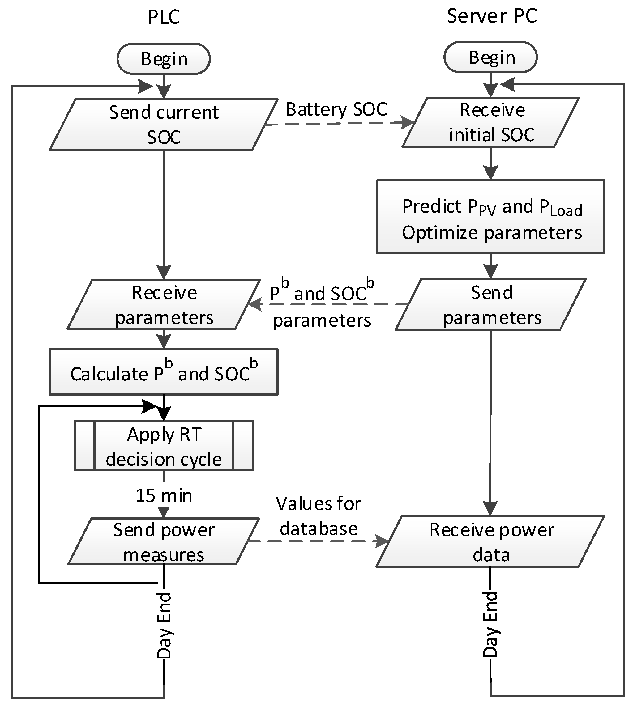
Figure 6.
Combined flow chart of the programmable logic controller (PLC) and Server PC (personal computer) duties.
Figure 6.
Combined flow chart of the programmable logic controller (PLC) and Server PC (personal computer) duties.

Figure 7.
Real hardware tests. (a) Devices power. Battery and load power are considered positive when received. Grid and PV power are considered positive when delivered. (b) Battery state of charge (SOC).
Figure 7.
Real hardware tests. (a) Devices power. Battery and load power are considered positive when received. Grid and PV power are considered positive when delivered. (b) Battery state of charge (SOC).

Figure 8.
Optimized SOCb and actual SOC evolution through the day.

Figure 9.
Predictions and actual values for (a) the PV generation and (b) the loads.

Figure 10.
Simulations results for the state-of-the-art method: (a) Devices power; (b) Battery SOC.


Table 1.
Suppliers and demanders priorities and allowed combinations.
| Supplier | 1: PV | 2: Bat B | 3: Grid A | 4: Bat A | 5: Grid B | |
|---|---|---|---|---|---|---|
| Demander | OSi or ODj | 1 | 3 | 4 | 6 | 7 |
| 1: Load | 8 | A | A | A | A | A |
| 2: Bat A | 5 | A | A | A | X | X |
| 3: Bat B | 2 | A | X | X | X | X |
Table 2.
Algorithm example.
| Device | OSi/ODj | R (kW) | P (kW) | |
|---|---|---|---|---|
| S1 | PV facility | 1 | 4 | 4 |
| S2 | Bat B | 3 | 0 | 0 |
| S3 | Grid A | 4 | 8.5 | 8.5 |
| S4 | Bat A | 6 | 5 | 0 |
| S5 | Grid B | 7 | 10 | 0 |
| D1 | Load | 8 | 12 | 12 |
| D2 | Bat A | 5 | 3 | 0.5 |
| D3 | Bat B | 2 | 2 | 0 |
Table 3.
Prices by day period.
| Price | 18:00–22:00 | 8:00–18:00 & 22:00–24:00 | 0:00–8:00 |
|---|---|---|---|
| CE k (€/kWh) | 0.018762 | 0.012575 | 0.004670 |
| CP k (€/kWmonth) | 3.384797 | 2.030890 | 1.353907 |
Table 4.
Cost comparison.
| Method | Energy Cost (€/month) | Power Cost (€/month) | Total Cost (€/month) |
|---|---|---|---|
| Proposed method | 23.3472 | 57.54155 | 80.8887 |
| Method from [22] | 26.8039 | 57.81233 | 84.6162 |
| Without battery | 30.2297 | 57.81233 | 88.0420 |
© 2019 by the authors. Licensee MDPI, Basel, Switzerland. This article is an open access article distributed under the terms and conditions of the Creative Commons Attribution (CC BY) license (http://creativecommons.org/licenses/by/4.0/).
Share and Cite
MDPI and ACS Style
Galván, L.; Navarro, J.M.; Galván, E.; Carrasco, J.M.; Alcántara, A. Optimal Scheduling of Energy Storage Using A New Priority-Based Smart Grid Control Method. Energies 2019, 12, 579. https://doi.org/10.3390/en12040579
AMA Style
Galván L, Navarro JM, Galván E, Carrasco JM, Alcántara A. Optimal Scheduling of Energy Storage Using A New Priority-Based Smart Grid Control Method. Energies. 2019; 12(4):579. https://doi.org/10.3390/en12040579
Chicago/Turabian StyleGalván, Luis, Juan M. Navarro, Eduardo Galván, Juan M. Carrasco, and Andrés Alcántara. 2019. "Optimal Scheduling of Energy Storage Using A New Priority-Based Smart Grid Control Method" Energies 12, no. 4: 579. https://doi.org/10.3390/en12040579
Note that from the first issue of 2016, this journal uses article numbers instead of page numbers. See further details here.