Driving Forces of Energy-Related CO₂ Emissions Based on Expanded IPAT Decomposition Analysis: Evidence from ASEAN and Four Selected Countries

Abstract

ASEAN is a dynamic and diverse region which has experienced rapid urbanization and population growth. Their energy demand grew by 60% in the last 15 years. In 2013, about 3.6% of global greenhouse-gas emissions was emitted from this region and the share is expected to rise substantially. Hence, a better understanding of driving forces of the changes in CO₂ emissions is important to tackle global climate change and develop appropriate policies. Using IPAT combined with variance analysis, this study aims to identify the main driving factors of CO₂ emissions for ASEAN and four selected countries (Indonesia, Malaysia, Philippines and Thailand) during 1971–2013. The results show that population growth and economic growth were the main driving factors for increasing CO₂ emissions for most of the countries. Fossil fuels play an important role in increasing CO₂ emissions, however the growth in emissions was compensated by improved energy efficiency and carbon intensity of fossil energy. The results imply that to decouple energy use from high levels of emissions is important. Proper energy management through fuel substitution and decreasing emission intensity through technological upgrades have considerable potential to cut emissions.

1. Introduction

Global warming is one of the most important current issues in the world due to its negative consequences to the environment. Human activity, particularly the consumption of energy, has been considered among the main factors contributing to the climate change in the past decades. According to the IPCC [1], “Human activities are estimated to have caused approximately 1.0 °C of global warming above re-industrial levels, with a likely range of 0.8 °C to 1.2 °C. Global warming is likely to reach 1.5 °C between 2030 and 2052 if it continues to increase at the current rate”. Nordhaus [2] also stated that “The ultimate source of global warming is the burning of fossil fuel (or carbon-based) fuels such as coal, oil, and natural gas, which leads to emissions of carbon dioxide (CO₂)”. The Association of Southeast Asian Nations (ASEAN) region is one that has experienced rapid population and economic growth with high energy dependency and also substantial increase in energy consumption and pollution emissions in recent years. Continuous urban growth has led to a changing of people’s life-styles and an improvement of their living standards which has stimulated energy consumption dramatically. Rapid economic and population growth since 2000, coupled with increasing urbanization has resulted in a strong rise in energy demand across the region, met primarily by fossil fuels. According to the IEA [3], energy demand in the region is expected to grow by about two-thirds by 2040, which represents a tenth of the global prediction, being the result of their economy that triples in size, and the total population that grows by a fifth with the urban population alone rising by more than 150 million people.

Primary energy demand in Southeast Asia grew by around 70% between 2000 and 2016 to around 640 million tons of oil equivalent (Mtoe), while its gross domestic product (GDP) more than doubled over the same period. Fossil fuels dominate the primary energy mix, accounting for almost 75% of the total in 2016. Oil continues to be the dominant source of energy, with the share of 34%, due to the increasing demand for mobility. Coal demand has more than tripled since 2000, with an annual average growth rate of 8.8%, to reach 110 Mtoe or 17% of total primary demand, of which the largest portion was for power generation. Abundant coal resources in the Southeast Asia region, as well as its relatively low cost, have underpinned the rise in coal demand, brought about by the policy imperatives to meet rising demand for electricity and extend access to electricity to millions of people. Natural gas consumption also grew rapidly, and reached a share of 22%, due to its’ increased use for power generation and industry. Solid biomass accounts for 20%. A variety of biomass, such as fuelwood, charcoal and agricultural waste is used as a source of energy, mainly in the residential sector, where it is relied on by around 250 million people for cooking. Though still high, the share of bioenergy in the mix has been in decline (it was about 26% in 2000) and this reflects the ongoing shift towards modern energy such as electricity (for lighting) and liquefied petroleum gas (LPG) (for cooking). IEA [3]

So far, the pollution in the region mainly comes from the combustion of coal for power generation and industrial process, followed by oil combustion, mainly in the transportation sector and urban emissions, mostly from the residential sector, of which 90% of the emissions from households result from the use of wood fuel and charcoal for cooking and heating. This is therefore a serious threat to air quality even though air quality standards are in place in some countries. Southeast Asia is extremely vulnerable to climate change with it’s extreme weather events (temperature, rainfall and storms) which impact both the energy demand and infrastructure of energy supply. About 80% of natural disasters are “hydrometeorological” events and these are expected to grow in number and severity with the effects of climate change. Average temperatures and rainfall are rising and sea levels in the region are expected to rise 10-15% more than the global average which could result in a one metre rise in some cities by the end of the century. World Bank [4]

Due to the importance of environmental issues to the economy, there have been a number of studies attempting to investigate the main driver to the environmental impact through the ‘IPAT’ model. This model, which was originally put forward in the 1970s, is an analytical tool for identifying the forces driving environmental impacts which was formulated by Ehrlich and Holdren [5]. It was used to illustrate how population (P), affluence (A), and technology (T) have acted as the key forces behind environmental impacts (I). Since the identity was developed, researchers have used this identity with modifications for a variety of reasons. For example, Soulé and DeHart [6] compared production-based and consumption-based atmospheric greenhouse-gas data in northwestern North Carolina and found that IPAT can be successfully used to examine the forces driving environmental impacts at the local scale.

Since 2000s, there has been a number of literature on index decomposition analysis, on which the IPAT model is based, for environmental emissions such as Ang and Zhang [7], Ang and Liu [8], and Ang et al. [9]. Moreover, IPCC [10] provided a comprehensive study and discussed the IPAT and the Kaya identity together with their application to future emissions scenarios covering a wide range of the main driving forces from demographic to technological and economic developments. The recent studies applying the decomposition IPAT model such as Raupach et al. [11] analysed the trends in emissions and demographic, economic, and technological drivers, by using the Kaya factors for the global/region levels (European Union, the nations of the Former Soviet Union, developed countries, developing countries, and least-developed countries) and the local level (U.S.A., Japan, China, India).

From 2010s, there has been a number of research work applying IPAT model on their energy and environmental studies at both national level (individual countries) and also comparative level (Multi countries/sectors). At the national level, for instance, Song et al. [12] conducted an analysis of China’s energy consumption using the expanded IPAT model and concluded that developing renewable energy and enhancing energy efficiency are crucial to economic growth and reduction of energy consumption in China. Linyun and Hongwu [13] studied the impact factors on CO₂ emissions in China for the periods 1980–2007 using the Kaya model. The results suggested that economic scale and energy saving are the main factors attributable to the changes of CO₂ emissions. In the future, energy efficiency factor is still likely to be the dominant role in controlling CO₂ emissions of the nation. Hubacek et al. [14], and Brizga et al. [15] investigated the driving forces of CO₂ emissions in China and the former Soviet Union, respectively. They confirmed that IPAT analysis can also be used to assess the different factors (energy intensity, affluence industrialization, energy mix, carbon intensity, and population) driving CO₂ emissions in these countries along the periods of the stages of economic development. Another study by Yue et al. [16], aimed to determine the optimal CO₂ reduction path for Jiangsu province to achieve the target of 40–45% reduction of CO₂ emissions intensity by 2020 based on the 2005 level, using the IPAT model combined with scenario analysis. They classified the determinants into four parameters: economic growth, population growth, energy intensity and renewable-energy share. The forecast results indicated that the province is likely to achieve the target. Rapid economic growth is the main factor that causes increase in CO₂ emissions, whereas the decrease of energy-intensity and the increase of renewable-energy-share, both have beneficial influences in reducing CO₂ emissions. For the comparative studies, Duro [17] attempted to assess the international inequalities in per capita CO₂ levels and the three Kaya factors (carbon intensities, energy intensities, and affluence) for various inequality indices and variety of sub-periods during the 1971–2007. Kaivo-oja et al. [18] investigated the factors that impact the amount of CO₂ emissions from fuel combustion and energy use in China, the EU-27, and USA using mathematical decomposition analysis. Moreover, Yao et al. [19] modified the IPAT framework to examine the main driving forces of CO₂ emissions in the G20 countries for the sub-periods in 1971–2010.

Many studies in the literature confirmed that IPAT model is an easily understandable, widely utilized framework for analyzing the driver of environmental change. It can be concluded that the index decomposition methods based on IPAT/ Kaya identity have been developed into two main groups: the ones based on the Laspeyre index and the ones based on the Divisia index. The most popular method based on the Divisia index is the Logarithmic Mean Divisia Index, the so called ‘LMDI’. There are some recent studies using this method. For example, Robaina-Alves et al. [20] analyzed what effects contribute more to CO₂ emissions in the Portuguese tourism sector for the period 2000–2008. The results show that tourism activity is the most important effect. Energy mix, carbon intensity and energy intensity effects are also important. Chen and Yang [21] decomposed the factors causing CO₂ emissions for 29 provinces in China over the periods 1995 to 2011. Twelve driving factors were decomposed into four categories of effects. The results are generally consistent among these regions. The average labor productivity is the main positive driving factor whereas the energy intensity of production sector is the dominant negative driving factor. The results suggest that China should coordinate and balance the relationships between economic development and CO₂ emission reduction, further decrease energy intensity of many production sectors, gradually adjust the economic and energy structures, and formulate CO₂ emission reduction policies to accommodate regional disparities. Although LMDI method seems to be widely used in the literature, there are some limitations in terms of handling negative and zero values in the environmental data set. To cover this point, Pani and Mukhopadhyay [22,23] proposed the technique so called ‘Variance analysis—A management accounting approach’ (which is basically developed from Kaya identity) to find the factors affecting CO₂ emissions in their studies. In the first study, the method is used to decompose the changes in CO₂ emissions among 156 sample countries over the period 1993–2007. The finding shows that in general both rising population and GDP per capita are the main driving forces to increase emissions while the reductions in energy and emission intensities, and substitution of fossil fuels by non-emitting ones are likely to decrease emissions. In the second study, this technique is used to analyse the carbon dioxide emissions of the top ten emitting countries over the period 1980–2007 in order to examine the determining factors. The main results indicate that even though the expansion of income and population are the dominant driving forces to increase emissions, energy structure and CO₂ emission intensities are also the crucial factors.

It is widely accepted that IPAT is a simple, systematic and robust model for analyzing the effect of human activities on the environment. IPAT specifies that environmental impacts are the multiplicative products of three key driving forces: population, affluence (per capita consumption or production) and technology (impact per unit of consumption or production), thus I = PAT. IPAT is a mathematical identity and has typically been used as an accounting equation. The main strengths of the model are that it is a parsimonious specification of key driving forces behind environmental change as it identifies precisely the relationship between those driving factors and impacts. However, the key limitation of IPAT is that the model does not permit hypothesis testing since the known values of some terms determine the value of the missing term. Moreover, they assume proportionality in the functional relationship between factors (York et al. [24]). This means that the elasticity of environmental impact with respect to P, A, T and other determinants is only one respectively, which indicates that each driving factor is equally important for the environmental impact in the model. To overcome this limitation, Dietz and Rosa [25,26] reformulated IPAT into a stochastic model, so called ‘STIRPAT’ for stochastic impacts by regression on population, affluence and technology. The model allows for non-monotonic or non-proportional effects from driving forces. Most STIRPAT researchers use the econometric framework as a starting point, and then specify model by simply adding or dropping variables so long as they are conceptually appropriate for its multiplicative specification. However, it was found in the literature that many have added other factors that might not satisfy this requirement. The lack of a unified standard and theoretical guidance in selecting variables combined with arbitrarily adding or removing of variables is likely to reduce the credibility and robustness of the model as the research results (even with the same objective) could show the last deviation due to the use of different variables. This would be a main drawback of the STIRPAT method. (Lin et al. [27]).

Regarding IPAT studies, there have been intensive studies on national CO₂ emissions decomposition, especially for the major developed economies, however, there is a lack of studies focusing on the CO₂ emissions from ASEAN countries. These ASEAN countries have a great potential for CO₂ emission growth in the future since many manufacturing activities are outsourced in developing countries because labor is cheaper. Moreover, by 2030, two-thirds of global middle class people are expected to live in the Asia Pacific region (Sumabat et al. [28]). Decomposition analysis is a method that looks into the driving force behind the changes of the CO₂ emission over time but few have been conducted on this subject. The most recent significant ones are the following. Resosudarmo et al. [29] attempted to decompose the CO₂ emissions from fossil fuels based on Kaya identity to find the main driver behind the increase of the emission in Indonesia for the period 1971–2004. The results indicate that CO₂ emissions from fossil fuel are still the dominant factor. Energy intensity and carbon intensity are the main drivers of the increase of the emissions. The main reason behind the increase of carbon intensity comes from the rapid increase in the use of coal as a source of energy especially in electricity sector. Sumabat et al. [28] quantified the driving forces of changes in Philippines CO₂ emissions from 1991 to 2014. The results show that the majority of the increases in CO₂ emissions come from economic activities due to life style change of the population. Moreover the results show a consistent improvements in energy intensity which is driven mainly by the shift in the primary sector from manufacturing to service.

There have been a very limited number of comparative ASEAN studies investigating the driving forces of CO₂ emissions. A study has been conducted by Nurdianto and Resosudarmo [30] but it focuses on the decomposition of energy rather than CO₂ emissions. They used Kaya’s identity method to analyse the energy patterns among ASEAN member countries in order to address the issues of ASEAN integration of energy policies. Another study conducted by the same authors in 2016 [31] aims to analyse the benefit and losses associated with cooperation among ASEAN members in mitigating their CO₂ emissions, particularly by implementing a uniform carbon tax accord ASEAN using CGE model. The most relevant study is conducted by Sandu et al. [32] who used decomposition analysis (the LMDI method) to analyse the historical development of CO₂ emissions and the underlining factors for the ASEAN countries in a period 1971–2009. The results imply that the main contributing factors of the increase of emission in the region come from level of affluences (per capita GDP), followed by fuel-mix effect (as emission-intensive fossil fuels increasing become dominant energy sources), population effect (due to high population growth in the region), and structural effect (as the regional production structure has increasingly concentrated on the energy-intensive industrial sector). On the other hand, the main dominant factors of the reduction of the emission are the intensity effects which comprise both end-use energy intensity and fuel conversion intensity. However, LMDI method has some drawbacks in terms of its incapability of handling negative and zero values in environmental data set (Pani and Mukhopadhyay [22,23], Wood and Lenzen [33]). Therefore to eliminate the problem, Chontanawat [34] adopted the IPAT method combined with variance analysis, based on Pani and Mukhopadhyay [22,23] to investigate the driving forces of CO₂ emissions for ASEAN (not specific to individual countries) for the longer period 1971–2013. It was found that population growth and increased income per capita have the largest contribution to emission growth; fossil fuels increasingly become the dominant fuel; energy efficiency and carbon intensity (emission factor) are the factors that reduced emissions. Due to insufficient past studies for ASEAN, this study aims to add to the literature by extending the research from Chontanawat [34] to further investigate the region and four selected Southeast Asian countries: Indonesia, Malaysia, Philippines and Thailand as a case study for the period 1971–2013. These countries are fast-growing, experiencing severe pollution, rising energy consumption and rapid urbanization. Even though they are slightly different in terms of scale and pattern of energy use and energy endowments, they share a common challenge to meet increasing demand in a secure, affordable and sustainable manner. It would be very interesting to understand the evolution of carbon emissions, energy consumption and economic growth, of these countries during the past decades and the linkages between these variables and the changes of their fuel mix, etc., through IPAT factors. Are the patterns similar or different among these individual countries? We focused on CO₂ emissions from fossil-fuel combustion, the dominant anthropogenic forcing flux. The results could provide suitable policy implications related to energy and environment in order to enhance energy security, to ensure affordability and to improve energy efficiency under the umbrella of sustainability. The remainder of the paper is organised as follows: Section 2 introduces the research methods and variable used. Section 3 provides the results and discussion. Finally, Section 4 gives conclusions.

2. Materials and Methods

To understand the magnitudes and patterns of the factors influencing CO₂ emissions in these countries, in this study, we analyse the driving forces by using IPAT decomposition method combined with Variance analysis for the periods 1971–2013. The main variables in the model comprise CO₂ emissions, energy consumption, population and Gross domestic products (GDP) of these countries. The CO₂ emissions and energy data are extracted from IEA 2015 database [35] whereas the population and GDP data are drawn from the World Bank’s World Development Indicators (WDI) [36].

2.1. IPAT Analysis

First, the IPAT factors: I, P, A, E, F, and C based on Kaya Identity are identified as follows:

$$I_i=P_i\times \frac{GD{P}_i}{P_i}\times \frac{PE{S}_i}{GD{P}_i}\times \frac{FE{C}_i}{PE{S}_i}\times \frac{I_i}{FE{C}_i}=P_i\times A_i\times E_i\times F_i\times C_i$$

(1)

where:

I	CO2 emission flux in Mt of CO2 emissions
P	population in million persons
GDP	real GDP: defined and measured at constant price in million 2005 USD
PES	primary energy supply in ktoe
FEC	fossil fuel consumption in ktoe
A	GDP per capita or affluence (A = GDP/P) in 2005 USD
E	energy intensity (E = PES/GDP) in ktoe per million 2005 USD
F	fuel mix (F = FEC/PES) in ktoe of fossil fuel consumption per ktoe of primary energy supply
C	CO2 per unit of energy (C = I/FEC) in Mt of CO2 emissions per ktoe
Subscript i	refers to the ASEAN region or countries; the ASEAN region comprises 10 countries; Brunei, Cambodia, Myanmar, Laos, Indonesia, Malaysia, Indonesia, Philippines, Vietnam and Thailand. Laos was excluded in the study due to the unavailability of the data

2.2. Variance Analysis

The word ‘variance’ used in the study is given by Pani and Mukhopadhyay [22,23] who first introduced this method in the emission studies. Variance analysis is the process of analyzing variance (the change) by subdividing the total variance (total change) in such a way that management can assign responsibility for off-standard performance. The variance analysis technique is originally used in the financial area to measure the change in total revenue/cost attributable to change in factors, those are total revenue/cost is expressed as a product of price/cost per unit and the total quantity of sale/production respectively.

To decompose the driving factors of CO₂ emissions, we adopted variance analysis technique introduced by Pani and Mukhopadhyay [22,23] and further used by Chontanawat [34]. This method is built upon based on the IPAT identity, where emission is shown as the product of its identities driving factors as mentioned earlier. The method is easy to understand and does not require much complicated mathematical or econometric technique. Furthermore, this method covers the advantages of the well-known LMDI approach, but has more capability to manage the residual terms. Ang [37] also addressed that the LMDI method fails to deal with the negative and zero values in the data set. In the emission studies, these kind of values could occur in the analysis. Although Ang et al. [38] recommended to compensate the zeroes by small positive constants, Wood and Lenzen [33], nevertheless, argued that substitution of the large number of zeroes could produce substantial errors.

The IPAT identity based upon index decomposition analyses allows identification of the relationship between the driving factors and environmental impacts. The idea of decomposition can be visualized as in Figure 1.

Figure 1 demonstrates the links of these driving factors which is expressed as the chain between the fundamental variables such as POP (population), GDP (gross domestic product), PES (primary energy supply), FEC (fossil fuel consumption), and CO₂. The links between these variables are represented as the five driving factors. For example, A (or GDP per capita) is derived from GDP divided by population. In the same way, E (or energy intensity) is derived from PES divided by GDP. F (or fuel mix) is derived from FEC divided by PES, and C or emission factor is derived from CO₂ divided by FEC.

Therefore the change of CO₂ emissions (∆I) between periods 0 and t (let say a base year 0 and a target year t) comes from the changes of five driving factors between the same period as shown in Figure 2.

In Figure 2, the change of the CO₂ emissions (which is so called ‘CO₂ emission variance’) is a combination of the changes of five driving factors. They are the change in population (so called ‘population variance’), the change in GDP per capita (so called ‘income variance’), the change in fuel mix (so called ‘substitution variance’), and the change in emission factor (so called ‘emission intensity variance’).

From the Kaya Identity in Equation (1), CO₂ emissions in region/country ‘i’ at time period ‘t’ can be expressed as Equation (2):

$$I_i\left(t\right)=P_i\left(t\right)\times A_i\left(t\right)\times E_i\left(t\right)\times F_i\left(t\right)\times C_i\left(t\right)$$

(2)

At time ‘t + 1′, the resulting emission ‘I_i ’ can be expressed as Equation (3):

$$I_i\left(t+1\right)=P_i\left(t+1\right)\times A_i\left(t+1\right)\times E_i\left(t+1\right)\times F_i\left(t+1\right)\times C_i\left(t+1\right)$$

(3)

An analysis of the difference between CO₂ emission in time ‘t’ and ‘t + 1′ is called ‘variance analysis’. The process decomposes the difference in five components: population variance, income (affluence) variance, energy intensity variance, substitution variance, and emission intensity variance. The following equation expresses the total variance of CO₂ emission between time ‘t + 1’ and ‘t’.

Total emission variance:

$$\Delta I_i\left(t\right)=\Delta P_i\left(t\right)+\Delta A_i\left(t\right)+\Delta E_i\left(t\right)+\Delta F_i\left(t\right)+\Delta C_i\left(t\right)$$

(4)

Equation (5) determines the change in emission due to population change, which is called ‘population effect’ or population variance. If there is a change in population, with other factors remaining constant, there must be a proportionate change in emission so that the population effect may be held solely responsible for this effect.

Population variance:

$$\Delta P_i\left(t\right)=\Delta P_i\left(t\right)\times A_i\left(t\right)\times E_i\left(t\right)\times F_i\left(t\right)\times C_i\left(t\right)=\left[P_i\left(t+1\right)-P_i\left(t\right)\right]\times A_i\left(t\right)\times E_i\left(t\right)\times F_i\left(t\right)\times C_i\left(t\right)$$

(5)

In the same way as population variance, the other variances can be expressed as follows:

Income variance:

$$\begin{array}{cc}\hfill \Delta A_i\left(t\right)=P_i\left(t+1\right)\times & \Delta A_i\left(t\right)\times E_i\left(t\right)\times F_i\left(t\right)\times C_i\left(t\right)\hfill \\ & =P_i\left(t+1\right)\times \left[A_i\left(t+1\right)-A_i\left(t\right)\right]\times E_i\left(t\right)\times F_i\left(t\right)\times C_i\left(t\right)\hfill \end{array}$$

(6)

Energy intensity variance:

$$\begin{array}{cc}\hfill \Delta E_i\left(t\right)=P_i\left(t+1\right)& \times A_i(t\hfill \\ & +1)\times \Delta E_i\left(t\right)\times F_i\left(t\right)\times C_i\left(t\right)=P_i\left(t+1\right)\times A_i\left(t+1\right)\hfill \\ & \times \left[E_i\left(t+1\right)-E_i\left(t\right)\right]\times F_i\left(t\right)\times C_i\left(t\right)\hfill \end{array}$$

(7)

Substitution variance:

$$\begin{array}{c}\Delta F_i\left(t\right)=P_i\left(t+1\right)\times A_i\left(t+1\right)\times E_i\left(t+1\right)\times \Delta F_i\left(t\right)\times C_i\left(t\right)=P_i\left(t+1\right)\times A_i(t\hfill \\ +1)\times E_i\left(t+1\right)\times \left[F_i\left(t+1\right)-F_i\left(t\right)\right]\times C_i\left(t\right)\hfill \end{array}$$

(8)

Emission intensity variance:

$$\begin{array}{l}\Delta C_i\left(t\right)=P_i\left(t+1\right)\times A_i\left(t+1\right)\times E_i\left(t+1\right)\times F_i\left(t+1\right)\times \Delta C_i\left(t\right)=P_i\left(t+1\right)\times A_i(t\\ \hspace{1em}\hspace{1em}\hspace{1em}\hspace{1em}\hspace{1em}\hspace{1em}+1)\times E_i\left(t+1\right)\times F_i\left(t+1\right)\times \left[C_i\left(t+1\right)-C_i\left(t\right)\right]\end{array}$$

(9)

3. Results and Discussion

3.1. Overview of ASEAN’s Emissions

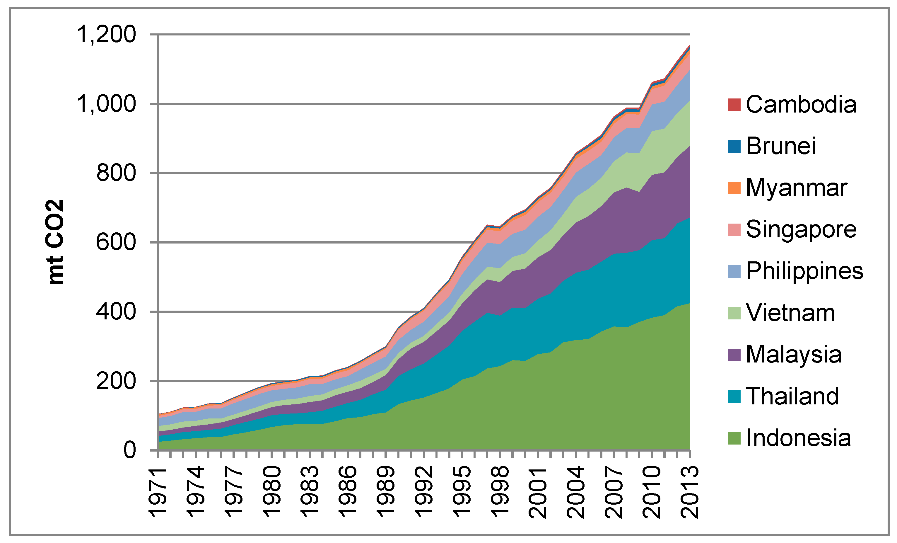
CO₂ emissions in ASEAN (excluding Laos as per Figure 3), show that emission rose rapidly over the period 1990–2013. In 2013, the largest emitters were Indonesia, followed by Thailand, Malaysia, Vietnam, Philippines, Singapore, Myanmar, Brunei and Cambodia.

In general, the ASEAN region is well-endowed with fossil fuels and renewable energy supply. Primary energy mix is dominated by fossil fuels, with oil, natural gas and coal making up more than three-quarters of demand. Over recent decades, there has been an ongoing shift towards coal and natural gas, primarily at the expense of oil in power generation and industry, and traditional biomass in the residential sector. However, oil is still the dominant fuel at about 35.5% share in the primary energy mix (in 2013), followed by natural gas with 22.5% share. Coal has been increasing at double digit rates since 1990 and has tripled it’s share of energy mix to 15.4%. Renewable energy contributed about 26.5% of energy mix. In this part, traditional biomass plays a major role in this share with the vast majority being used for cooking by people living in rural areas with low incomes and/or a lack of infrastructure restricting their use of modern fuels. (see Figure 4).

Figure 5 demonstrates the ASEAN countries’ contemporary aspects in terms of cumulative fossil fuel emissions, the emission level in the current year (2013), the emission growth, and the share of population in the current year (2013). It can be seen that Indonesia, Thailand, Malaysia and Philippines are the top four CO₂-emitting countries during 1971–2013. Indonesia has the largest population share (41% of the ASEAN’s population). This is in line with their largest share of CO₂ emission levels (about 36% of ASEAN) both in that year and throughout the whole period from 1971-2013. However, during the past decade their emissions grew by on average only 3.5%, lower than other ASEAN countries such as Cambodia, Vietnam and Brunei which increased by about 8.7%, 6.4%, and 4.5%, respectively.

When considering the CO₂ released from different types of energy used (CO₂ emission flux from fossil fuel combustion) in these ASEAN countries, it includes contributions from the following main sources: national-level combustion of coals, oil, and natural gas. Hence:

$$FEC=F_{Coal}+F_{Oil}+F_{Natural gas}$$

(10)

The contribution of each source to the total FEC (Fossil energy consumption) is indicated in Figure 6. For the ASEAN, CO₂ emissions from oil, coal and peat, and natural gas accounted for 44%, 32%, and 24% respectively. The main emitter was Indonesia followed by Thailand, Malaysia, Vietnam and Philippines.

When looking at the share of CO₂ emitted from different energy sources in each particular country (across the individual countries) which is shown in Figure 7, the majority of CO₂ released in these countries come from the use of oil and coal except for Brunei where the main source of emissions come from natural gas.

In summary, CO₂ emissions in the region increased substantially during 1971–2013. The next section will analyse the main driving factors behind the change of CO₂ emission over this period through IPAT model combined with variance analysis for ASEAN and four selected countries (Indonesia, Malaysia, Philippines and Thailand).

3.2. Results from IPAT analysis

According to the IPAT identity which is expressed as I = P × A × E × F × C (where P = pop, A = GDP/Pop, E = PES/GDP, F = FEC/PFS, and C = CO₂/FEC), the trends of these driving factors in ASEAN emissions and the four selected national emissions (Indonesia, Malaysia, Philippines and Thailand) for 1971–2013 are shown in Figure 8. All quantities are normalized to 1 in the year 1971 to show the relative contributions of changes in Kaya factors to changes in emissions. It can be seen that the increase in the growth rate of the CO₂ emission (I) is a combination of the increase of population (P), per capita GDP (A), fuel mix (F), and the reductions of energy intensity (E) and emission intensity of energy (C), and also that the trends of ASEAN and the four individual countries are generally increasing.

Table 1. Values of IPAT variables in ASEAN and four selected countries in 2013

Countries	Population (P)	Affluence (A)	Energy Intensity (E)	Energy Mix (F)	Emission Factor (C)	CO2 Emissions (I)
(Unit)	million	US$/POP	toe/1,000US$2005	toe FEC/toe PES	mt CO2/mtoe PES	mt CO2
Indonesia	250.00	1,788	0.48	0.66	3.01	424.61
Malaysia	29.72	7,052	0.43	0.95	2.46	207.25
Philippines	98.39	1,591	0.29	0.61	3.28	89.63
Thailand	67.01	3,752	0.53	0.80	2.29	247.45
ASEAN	607.71	2,263	0.43	0.73	2.69	1,170.92

shows the values (without normalization) of the driving force factor in 2013. It can be seen that, Indonesia is the biggest producer of CO₂ in the region, followed by Thailand, Malaysia and Philippines. In terms of population, Indonesia also is the largest country. The second is Philippines, followed by Thailand and Malaysia. This affects the level of GDP per capita which shows that Malaysia has the highest per capita income, double that of Thailand and quite far behind the rest. Energy intensity of Thailand (0.53) and Indonesia (0.48) are higher than the average of ASEAN (0.43), while Malaysia (0.43) remains the same and Philippines (0.29) is the lowest. In terms of fuel mix level, most of the countries in the region still rely on fossil fuel (the shares of fossil fuel in total energy are greater than 60%). For the emission factor or emission intensity of energy which represents the quality of fuels used, Philippines and Indonesia have a high ratio (3.28, and 3.01) which is greater than the average for ASEAN (2.69), whereas Malaysia and Thailand have lower ratio (2.46, and 2.29) than the average of ASEAN.

The following section will analyse the contribution of the changes of CO₂ emissions via IPAT factors over the period 1971–2013. This can be undertaken by ‘Variance Analysis’ method.

3.3. Results from Variance analysis

This section shows the results drawn from the Variance analysis for the ASEAN and the four selected countries. The results are demonstrated in Figure 9, Figure 10, Figure 11, Figure 12 and Figure 13 and also Appendix A.

3.3.1. ASEAN Analysis

The ASEAN CO₂ emission decomposition results is shown in Figure 9 (see also Appendix A: Figure A1 and

Table A1. Decomposition results of total CO₂ emissions in ASEAN and selected countries (Mt CO₂).

Country	Indonesia					Malaysia					Philippines
	1971–1980	1981–1990	1991–2000	2001–2013	1971–2013	1971–1980	1981–1990	1991–2000	2001–2013	1971–2013	1971–1980	1981–1990	1991–2000	2001–2013	1971–2013
Change in total emission (∆CO2)	42.39	60.81	113.60	146.92	399.38	10.90	23.86	54.58	87.88	194.45	10.32	6.41	30.78	21.74	66.59
Population variance	6.32	14.74	21.10	47.67	28.50	3.03	7.21	14.98	27.67	20.91	6.58	8.59	8.48	15.32	37.91
Income variance	18.71	37.57	35.03	204.92	225.21	9.88	9.81	33.44	69.66	132.83	9.19	−4.07	3.99	41.15	53.66
Energy intensity variance	−10.17	−2.45	16.86	−157.90	−125.29	−0.19	1.28	0.01	−10.55	21.50	−5.13	4.15	2.28	−45.28	−47.62
Substitution variance	33.77	16.61	28.32	27.08	256.80	3.05	1.70	3.80	3.31	48.88	−1.97	−1.56	10.34	10.10	12.39
Emission intensity variance	−6.23	−5.66	12.29	25.14	14.16	−4.87	3.86	2.34	−2.20	−29.68	1.65	−0.70	5.70	0.45	10.24
Country	Thailand					ASEAN exc. Laos
	1971–1980	1981–1990	1991–2000	2001–2013	1971–2013	1971–1980	1981–1990	1991–2000	2001–2013	1971–2013
Change in total emission (∆CO2)	17.49	48.34	62.27	87.45	231.21	89.10	156.39	308.48	440.00	1065.12
Population variance	4.03	5.55	8.60	10.18	12.61	25.35	42.33	61.72	117.60	119.84
Income variance	9.78	27.33	28.87	99.29	142.51	76.41	98.29	141.67	512.66	944.34
Energy intensity variance	−3.95	−4.05	15.38	18.89	−12.32	−48.10	−24.04	6.00	−260.91	−510.59
Substitution variance	4.59	19.29	29.96	−2.72	136.95	43.04	46.73	94.84	82.90	593.38
Emission intensity variance	3.04	0.21	−20.53	−38.19	−48.54	−7.59	−6.92	4.26	−12.25	−81.84

Note: The highlight columns represent the values for the whole periods (1971–2013).

and

Table A2. Decomposition results of total CO₂ emissions in ASEAN and selected countries (Share).

Country	Indonesia					Malaysia					Philippines
	1971–1980	1981–1990	1991–2000	2001–2013	1971–2013	1971–1980	1981–1990	1991–2000	2001–2013	1971–2013	1971–1980	1981–1990	1991–2000	2001–2013	1971–2013
Change in total emission (∆CO2)	1.00	1.00	1.00	1.00	1.00	1.00	1.00	1.00	1.00	1.00	1.00	1.00	1.00	1.00	1.00
Population variance	0.15	0.24	0.19	0.32	0.07	0.28	0.30	0.27	0.31	0.11	0.64	1.34	0.28	0.70	0.57
Income variance	0.44	0.62	0.31	1.39	0.56	0.91	0.41	0.61	0.79	0.68	0.89	−0.64	0.13	1.89	0.81
Energy intensity variance	−0.24	−0.04	0.15	−1.07	−0.31	−0.02	0.05	0.00	−0.12	0.11	−0.50	0.65	0.07	−2.08	−0.72
Substitution variance	0.80	0.27	0.25	0.18	0.64	0.28	0.07	0.07	0.04	0.25	−0.19	−0.24	0.34	0.46	0.19
Emission intensity variance	−0.15	−0.09	0.11	0.17	0.04	−0.45	0.16	0.04	−0.03	-0.15	0.16	−0.11	0.19	0.02	0.15
Country	Thailand					ASEAN exc. Laos
	1971–1980	1981–1990	1991–2000	2001–2013	1971–2013	1971–1980	1981–1990	1991–2000	2001–2013	1971–2013
Change in total emission (∆CO2)	1.00	1.00	1.00	1.00	1.00	1.00	1.00	1.00	1.00	1.00
Population variance	0.23	0.11	0.14	0.12	0.05	0.28	0.27	0.20	0.27	0.11
Income variance	0.56	0.57	0.46	1.14	0.62	0.86	0.63	0.46	1.17	0.89
Energy intensity variance	−0.23	−0.08	0.25	0.22	−0.05	−0.54	−0.15	0.02	−0.59	−0.48
Substitution variance	0.26	0.40	0.48	−0.03	0.59	0.48	0.30	0.31	0.19	0.56
Emission intensity variance	0.17	0.00	−0.33	−0.44	−0.21	−0.09	−0.04	0.01	−0.03	−0.08

Note: The highlight columns represent the values for the whole periods (1971–2013).

)). The results show the rising of CO₂ emissions in 1971–2013 of 1,065.12 Mt of CO₂. The factors contributing to the increase of emission were income effect (GDP per capita or affluence), substitution effect, and population effect, whereas the energy intensity effect and emission intensity effect (carbon intensity) help to reduce the emission. The income effect accounts for 944.34 Mt of CO₂, contributing the most to the change of CO₂ (89% in share), followed by substitution effect: 593.38 Mt of CO₂ (56%), population effect: 119.84 Mt of CO₂ (11%). While the energy intensity effect decreases the CO₂ emissions for 510.59 Mt of CO₂ (–48%), followed by emission intensity effect: 81.84 Mt of CO₂ (–8%). These results are consistent with Chontanawat [34] and similar to Sandu et.al [32] in that the main driving factors were affluence, fuel-mix, and population respectively, while end-use efficiency and carbon coefficient were the offset factors in CO₂ emissions.

The results indicated that affluence or GDP per capita is the most crucial factor in increasing CO₂ emission of the region where their economy has been growing rapidly. The contribution of substitution effect, which is about half, indicates that the region still depends on fossil fuels and this effect increases CO₂ emissions quite substantially. The results from the study also show the interesting point that energy intensity effect is likely to be the most significant factor to decrease CO₂ emissions in the region. Especially in the last decade, this effect has substantially contributed to CO₂ reduction for 260.91 Mt of CO₂ (59% in share). During this sub-period energy intensity declines quite dramatically (compared with the previous period) with negative growth. This led to the reduction in emission of 510.59 Mt of CO₂ (48% in share) for the entire period. The intensity ratio would continue to decline if ASEAN reached their goal under the Asia Pacific Economic Cooperation (APEC) Green Growth, that being an aspirational goal in the reduction of aggregate energy intensity by 45% by 2035 (based on 2005 level) [39]. The contribution of emission factor in terms of share is rather small but it shows improvement in helping reducing CO₂ emissions particularly in the last sub-period.

3.3.2. Country Analysis

Indonesia

The decomposition results (Figure 10, and see also Appendix A: Figure A1 and Table A1 and Table A2) show that, there had been a continued increase in emission change from 1971 to 2013. The change was 399.38 Mt of CO₂ increase in energy-related emission. CO₂ emissions increased due to the rise in substitution of fossil fuel, per capita GDP, population, and emission intensity were about 256.80 Mt of CO₂ (64% in share), 225.21 Mt of CO₂ (56%), 28.50 Mt of CO₂ (7%) and 14.16 Mt of CO₂ (4%) respectively. Energy intensity accounted for 125.29 Mt of CO₂ (–31%) of CO₂ emission reduction.

The empirical results show that the major contributing driving factor in CO₂ emissions in Indonesia during 1971-2013 is the substitution effect (fuel mix effect) which mean that the economy still mainly rely on the use of fossil fuel, followed by income effect and population effect. The contribution of income effect (Income variance) throughout the whole period continued to climb and had a big jump in the last sub-period. This is because their economy had recovered from the ASEAN financial crisis. The contribution of population effect which even though not large but continued to grow. The contribution of energy intensity and emission (carbon) intensity are important. There was a shift in the country to use more polluted energy source. Natural gas and oil consumption were being gradually replaced by coal in the last decade, that caused an increase in CO₂ emission from coal to about 32% of total CO₂ emissions in 2013 (IEA) [40]. Coal is the most emission intensive fossil fuel, followed by oil, then gas. Coal released roughly twice the amount of CO₂ per unit of energy than gas, depending on the quality of fuel and combustion technology (Resosudarmo et al. [29]).

In general, the results are in line with the Resosudarmo et al. [29] who study the kaya driving factors of CO₂ but in the earlier period 1971–2004, in the sense that apart from the economic activity that drove CO₂ emissions, the high proportion of fossil fuels in energy mix is also significant. This could affect the level of energy intensity and carbon intensity. Energy intensity and carbon intensity are the main drivers of the increase of the emission. The results are also consistent with Sandu et al. [32] who studied for a longer period (1971–2009) than Resosudarmo et al. [29], but a shorter period than ours (1971–2013). The results imply that the main contributing factors on CO₂ emissions are economic activities, the reliability on fossil fuel, the high intensity of energy and carbon intensity in the economy.

Malaysia

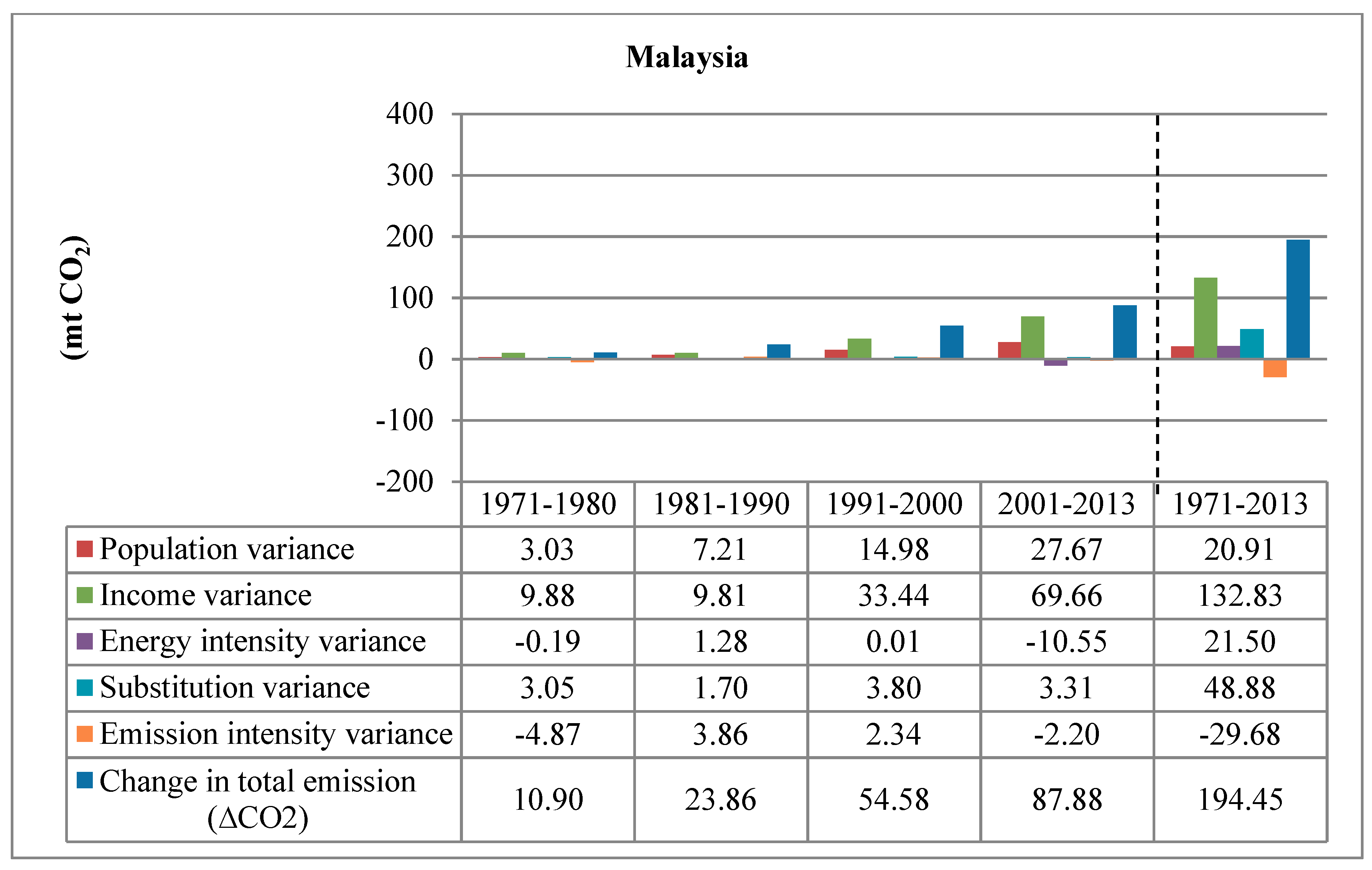
Figure 11 (and see also Appendix A: Figure A1 and Table A1 and Table A2) shows decomposition results of total CO₂ in energy-related emission in Malaysia during the period 1971 to 2013. The changes were rising along sub-periods with the average of 194.45 Mt of CO₂ for the entire period. Unlike Indonesia, the income effect accounted for 132 Mt of CO₂: the largest share of increasing CO₂ emissions (68%), followed by substitution effect: 48.88 Mt of CO₂ (25%), energy intensity effect: 21.50 Mt of CO₂ (11%), and population effect: 20.91 Mt of CO₂ (11%), while emission intensity effect contributed to the decrease CO₂ for 29.68 Mt of CO₂ (–15% in share).

The decomposition of increase in Malaysia’s CO₂ emissions shows that the largest emission-increasing factor throughout the period was GDP per capita. This income effect is shown by the high value number of income variance which was 132.83 Mt of CO₂ for the whole period 1971–2013. This effect was about six times larger than the population effect. The fossil fuel consumption which is represented by the substitution variance was the second largest portion (48.88 Mt of CO₂), and it had a positive impact on CO₂ emissions throughout all sub-periods. The last push effect is energy intensity (21.50 Mt of CO₂) which, however, had a fluctuating direction for the sub-periods. It can be seen that the variances were negative in the 1970s and change to positive in the 1980s and 1990s and then return to be negative again in 2000s. This was probably due to the increasing consumption of oil for transport, and coal and natural gas for electricity generation particular in 1980s and 1990s. However during 2000s, the government implemented the energy efficiency (EE) program under the eight Malaysia Plan 2001–2005 [41] to promote the efficient utilization of energy focusing on the industrial and commercial sectors. The direction of the contributing drivers seems to be consistent with the work of Sandu et al. [32]. Emission intensity variance has the same direction as energy intensity and has a negative value of (−29.68 Mt of CO₂). This indicates that the reduction of the change in emission intensity would help to reduce CO₂ emissions.

Philippines

From Figure 12 (and see also Appendix A: Figure A1 and Table A1 and Table A2), it can be seen that the change in total emission in Philippines between 1971 and 2013 caused an increase to 66.59 Mt of CO₂. The main contributing driver was income per capita then population, fossil fuel consumption (substitution), and emission intensity which accounted for 53.66, 37.91, 12.39, and 10.24 Mt of CO₂ or (81%, 57%, 19%, and 15% in share), respectively. On the other hand, the decrease in energy intensity caused a decrease in CO₂ emissions (−47.62 Mt of CO₂ or −72% in share).

Like the results of other countries, the population effects had been positive throughout the period and tend to be increasing in all sub-periods. The income effect was the main driving force and gave a positive impact for all the periods except the 1980s when there was a political and economic crisis in the Philippines in the early 1980s (Solon and Floro [42]), which cause a decrease in per capita income. This led to the rise of energy intensity in that period. Decreasing in GDP per capita as well as energy intensity and emission factor all caused a drop in the change of CO₂ emissions in the 1980s. Afterwards, the economy recovered as shown from growth of GDP per capita and together with the increase in emission factor drove the CO₂ emissions upward in 1990s. Since 2000s, after the ASEAN financial crisis in 1997, the country has shown better performance. The energy intensity, fossil fuel share and emission factor have decreased which indicates the improvement in energy efficiency and less reliance on fossil fuels with better quality of fuels. Energy intensity was likely to be an important factor to reduce the country’s emission since 2000s and the reduction was over forty Mt of CO₂ (−45.28) during this period. This led to the decrease of CO₂ (−47.62 Mt of CO₂) for the whole period. Fossil fuel share or substitution variance contribute only 12.39 Mt of CO₂ (19%) for the entire period, which is the least compared with Indonesia, Malaysia and Thailand. This is probably due to the fact that Philippines is the only ASEAN nation that does not rely heavily on fossil fuel in the electricity sector, (Nurdianto and Resosudarmo [30]). For the emission intensity effect, it contributed least to the increase of total CO₂, 10.24 Mt of CO₂ (15% in share) for the entire period. It was noticed that there was an improvement in the last decade (with the share of this effect being only 2% compared with the previous decade of almost 20%).

Since 2000s, the Philippines initiated the 20 year energy roadmap to develop sustainable energy systems and access to clean and green energy, under the National Renewable Energy Program (NREP) [43]. This was launched in June 2011 and aimed to increase the renewable energy (RE) installed capacity to 15,304 MW by the year 2030 (an aspirational target), which is almost triple the 2010 base year level. This would result in a change in fuel substitution to use more clean energy, and lead to the reduction in total CO₂ emissions of the country.

The results are in line with Sandu et al. [32] and Sumabat et al. [28] in that economic growth together with the lifestyle change of the population is the main driver to the increase of CO₂ emissions. Philippines has been performing well in the past few years and, more than half of their CO₂ increase comes from the increase in economic activity. Energy intensity appears to have improved since 2003. This could be attributed of the service sector, which has less energy intensity compared to the industrial sector (Sumabat et al. [28]).

Thailand

The decomposition results (Figure 13 and see also Appendix A: Figure A1 and Table A1 and Table A2) show that overall there had been (231.21 Mt of CO₂) increase in energy-related emission during the period 1971–2013. This was mainly due to rises in per capita GDP, the substitution of fossil fuel, and population at about 142.51 Mt of CO₂ (62% in share), 136.95 Mt of CO₂ (59%), and 12.61 Mt of CO₂ (5%) respectively. However the increase of CO₂ was offset by the reduction of emission intensity and energy intensity by (−48.54 Mt of CO₂ (−21%) and −12.32 Mt of CO₂ (−5%). The decomposition of the increase in Thailand’s CO₂ emissions shows that the population effect has been positive and increasing even though slight, whereas the income effect has been the largest emission-increasing factor throughout the period. On average, the income effect is more than eleven times that of the population effect, and that effect has been sharply increasing since the 2000s. This indicates that GDP is the more dominant driving force behind emissions. Regarding the energy intensity effect, even though its’ contribution is not that large (−5%) (with different directions in sub-periods), it does help to reduce emissions of the country. This could indicate that the country has to some extent better energy efficiency. However, the substitution effect are positive for the aggregate period which implies an increase in the share of fossil fuel in energy use in general. However, in the last sub period 2001–2013, it becomes negative for the first time which implies some improvement in fuel mix. The last factor, emission intensity, has larger negative numbers for sub-periods from 1990s to the present. This indicates that there has been a continuous shift towards less emitting energy. Thailand has a larger share of clean fossil fuel but still consume more in energy in general.

The results are consistent with Sandu et al. [32] in that per capita income is the main driving force to increase CO₂ in Thailand followed by fuel mix effect. However, the contribution of emission factors effect helps to reduce CO₂ and the proportion is larger than ASEAN countries such as Indonesia, Malaysia and Philippines.

Thailand has launched an important energy policy in the last decade. The Energy Efficiency Plan 2015–2036 (EEP 2015) [44] has been implemented to promote every sector to consume energy efficiently. The target is to reduce energy intensity (EI) by 30 percent from 2010 to 2036. Moreover, the Alternative Energy Development Plan (AEDP 2015) [45] which has been revised to cover the periods 2015–2036 is also implemented. The aim is to encourage fossil fuel substitution by alternative energy, for example: to use biofuel to replace gasoline and diesel, to use biomass to replace kerosene or coal, etc. The main target of the new AEDP is to increase the portion of renewable energy either in the form of electricity, heat and biofuels to 30 percent of final energy consumption in 2036. The main objective of these plans is to encourage the country to use energy more efficiently and consume more renewable energy. However, it may take some time for the country to adjust their fuel consumption to be in line with the plans.

3.4. Discussion and Policy Implication

The overall results indicate that affluence or income per capita is the most significant factor in rising CO₂ emissions in the ASEAN region where their economies are growing rapidly. The substitution effect which, in general, accounts for about half implies that the region still relies on fossil fuels and this affects the increase of CO₂ emissions quite significantly. This is supported by the results of Nurdianto and Resosudarmo [30] which indicated that energy consumption is dominated by oil and gas with increasing use of coal in Indonesia, Malaysia, Philippines, Thailand and Vietnam. Energy intensity effect, on the other hand, seems to be the most crucial factor to reduce CO₂ emissions in the region. The contribution from the emission factor even is small but shows an improvement in reducing CO₂ particular for Thailand and Malaysia. This is probably due to the clear initiatives within the national energy policy and planning programmes, especially in the last decade. The results are generally consistent with the previous studies such as Resosudarmo et al. [29], Sandu et.al [32], Sumabat et al. [28], and Chontanawat [34].

In summary, the results imply that energy efficiency and the fuel mix adjustment to use more renewable energy together with encouraging low carbon technology seem to be the most effective ways to reduce emissions of the region in the future. In fact, ASEAN has large population and economic expansion, which inevitable causes an increase in the use of energy, and this could create a higher level of CO₂ emissions of the region. ASEAN has abundant energy resources both fossil energy and renewable energy. Fossil is still the dominant fuel used in the region, but it could be depleted in the future. There is a huge potential for renewable energy to be developed. In fact, ASEAN is richly endowed with diverse renewable energy sources. Solar and wind are considered to be the most promising form of renewable energy for urban areas (ASEAN Centre for Energy: ACE) [46]. There is a significant use of wind power in Indonesia, Thailand, Vietnam and Philippines, whereas, solar and biomass are likely to be promising in Thailand and Malaysia.

During the last two decades, many countries in ASEAN have implemented policies and programs to improve energy efficiency of end-users. These EE programs have been directed toward increasing energy and electricity efficiency in residential and commercial buildings, while others are directed toward increasing energy efficiency in energy intensive industry or transport. These policies and programs on EE&C have successfully created awareness and educated the market on the benefits of implementing energy efficiency activities. Moreover, ASEAN Member States (AMS) has set a goal to reduce overall energy intensity in ASEAN by 20% by 2020 and 30% by 2035 based on 2005 levels, through various activities. Furthermore, ASEAN collectively aim to secure 23% of their primary energy from modern, sustainable, renewable energy sources by 2025 (ACE) [46]. The renewable energy and energy efficiency targets of the four selected countries are shown in

Table 2. Renewable energy and energy efficiency targets in four selected ASEAN countries

Country	Renewable Energy and Energy Efficiency Targets	Reference Document (year)
Indonesia	Reduce energy consumption in 2025 by 17% in industry, 20% in transportation, 15% in household, 15% in commercial buildings as compared to business as usual. 23% renewable share of TPES (around 92.2 Mtoe in 2025), which consists of 69.2 Mtoe (45.2 GW) for electricity and 23 Mtoe for non-electricity. 31% renewable share in 2050	National Energy Policy (Government Regulation No. 79/2014)
Malaysia	Reduce electricity consumption by 8% in 2025 as compared with business as usual	National Energy Efficiency Action Plan (2014)
	Renewable energy installed capacity of 2080 MW (excluding large hydro) by 2020 contributing to 7.8% of total installed capacity in Peninsular Malaysia and Sabah.	National RE Policy and Action Plan (2011) and 11th Malaysia Plan 2016–2020 (2015)
Philippines	Reduce TFEC by 1% per year as compared with business as usual until 2040, equivalent to the reduction of one-third of energy demand Reduce energy intensity (TFEC/GDP) by 40% in 2040 as compared to 2005 level	Energy Efficiency Roadmap for the Philippines, 2017–2020 (2017)
	15.3 GW renewable energy installed capacity in 2030: Renewable energy additional targets: - Additional biomass capacity of 277 MW in 2015 - Additional wind capacity of 2345 MW in 2022 - Additional hydro of 5398 MW in 2023 - Additional ocean energy capacity of 75 MW in 2025 - Additional solar capacity of 284 MW in 2030 - Additional geothermal capacity of 1495 MW in 2030	National Renewable Energy Program Roadmap 2010-2030 (2010)
Thailand	Reduce energy intensity (TFEC/GDP) by 30% in 2036 compared with 2010 level	Thailand Energy Efficiency Policy 2015 Plan (2015)
	30% renewable energy in total energy consumption by 2036, in the form of electricity (20.11% in generation, approximately 19684 MW), heat (36.67% of heat production, approximately 25088 ktoe) and biofuels (25.04% in transportation sector, approximately 8712.43 ktoe)	Alternative Energy Development Plan (2015)

Source: Irena 2018 [47].

.

Each country has set some forms of renewable energy target, motivated by a range of factors. A key factor is ‘environmental protection and climate change mitigation’, particularly since, as part of the Paris Agreement, each country submitted nationally determined contribution (NDCs) to reducing the impacts of climate change. To reduce overall emissions, they require the support of energy-efficiency measures and accelerated renewable energy deployment. The second key factor is ‘energy security’. The oil and gas resources that traditionally dominate in energy mix particular in Indonesia and Thailand are beginning to decline. Therefore, Indonesia, for instance, has set a target of 23% and 31% of renewable energy in its primary energy supply mix in 2025 and in 2050. Thailand has set a target of 30% renewable energy in total energy consumption by 2036 with different breakdowns in each sector, for example, biofuels are expected to supply 25% of energy demand in transportation sector, and the share of renewables in electricity and heat is expected to reach 20% and 37% respectively. Another significant factor is ‘cost-competitiveness’. The increasing cost-competitiveness of renewable energy technologies is prompting countries to increase their adoption in their energy mix. Renewables-based electricity is cost competitive with traditional power sources and it is expected to become increasingly affordable across a wider range of countries and markets. For example, in Philippines, utility-scale solar power purchase agreements (PPAs) were signed in the country in 2017 for USD 0.06 kWh. The purchasing utility listed diversifying supply and bringing down electricity rates as the key drivers behind this agreement. This is reflected in the nation’s target to install 15.3 GW of renewable energy capacity by 2030, accounting for 61% of the projected electricity demand (IRENA 2017 [48]). The last important factor is ‘socio-economic benefits’. The countries are finally expected to achieve socio-economic benefits including job creation and income generation and access to affordable, clean and reliable energy for the large energy-poor population.

Although these four countries seem to have ambitious national targets to improve energy efficiency and promote renewable energy (compared with other ASEAN countries), there are some constraints to the development of renewable energy, including geographical, Institutional and investment factors (particular in Indonesia) [49]. Moreover the limited information on renewable energy technologies, lack of awareness, and limited private sector engagement would be major barriers to sustainable renewable energy development (especially in Malaysia) [50].

Hence, to achieve the set targets, countries need to develop clear policy frameworks and robust institutions and taken steps toward the liberalization of energy markets to encourage competitiveness in the sector. Adopting energy efficiency, investing in renewables and building capabilities on nuclear energy safety may be crucial for Southeast Asia to realise a low-carbon ASEAN Community consistent with the goals of the Paris Climate Agreement. The in-depth policy analysis for ASEAN should be investigated in the next research.

4. Conclusions

The main objective of this study is to understand the driving forces of CO₂ emissions on the ASEAN economies and four particular countries: Indonesia, Malaysia, Philippines, and Thailand. What are the main contributing factors to the changes of the CO₂ emissions in these countries? To answer the question, a decomposition method based on IPAT combined with variance analysis was employed for the period 1971–2013. The decomposition analysis of ASEAN and the four countries provides interesting results about the factors explaining change in the CO₂ emissions. In general, growth in income level and population are the major driving forces of emissions with the income effect being much stronger than the population effect and increasing over time. The population effect is not directly affected by the number but by its affluence (GDP per capita), while the income effect is not the same across countries. However, rising population and affluence cause an increase in emissions but the higher income does not necessarily generate a proportional rise in emissions. Energy mix effect is also a crucial contributing factor in increasing CO₂ in all countries, which implies that most of the ASEAN economies still rely on fossil fuel consumption rather than renewal energy. The offsetting factor, the energy intensity effect is found to be predominant followed by the emission intensity effect. This implies that the economy of the region still relies on fossil fuels which generate high emissions, therefore an improvement in the quality of fuels used is needed. With the unavoidable growth in population and pursuit for economic growth it is therefore necessary to find ways of arresting emission, via technological aspects and national policies to reduce energy and emission intensity and substitution of more emitting fuel by alternative energy. Although the results indicate that improvement in the offsetting effect by reducing energy intensity seems to be the most effective choice, in the context of the present energy intensive production, it is hardly feasible to reduce energy consumption to any level. Hence it is important to decouple energy use from a higher level of emission. The study shows that fuel substitution and a decreasing of emission intensity of each fuel through continuous technological up-grades have considerable potential to cut emissions. Proper energy management is likely to be the best way to sustain a higher level of economic growth with the present growth in population. Therefore, the clear policy frameworks and robust institutions together with steps taken toward the liberalization of energy markets to encourage competitiveness in the sector are crucial. This should be investigated in the future research.

References

- Intergovernmental Panel on Climate Change (IPCC). Global Warming of 1.5 °C. An IPCC Special Report on the Impacts of Global Warming of 1.5 °C above Pre-Industrial Levels and Related Global Greenhouse Gas Emission Pathways, in the Context of Strengthening the Global Response to the Threat of Climate Change, Sustainable Development, and Efforts to Eradicate Poverty; World Meteorological Organization: Geneva Switzerland, 2018. [Google Scholar]
- Nordhaus, W.D. The Climate Casino: Risk, Uncertainty, and Economics for a Warming World; Yale University Press: New Haven, CT, USA, 2015. [Google Scholar]
- International Energy Agency (IEA). Southeast Asia Energy Outlook 2017; World Energy Outlook Special Report; International Energy Agency: Paris, France, 2017; ISBN 9789264285576. [Google Scholar]
- World Bank. Turn Down the Heat: Climate Extremes, Regional Impacts, and the Case for Resilience. A report for the World Bank by the Potsdam Institute for Climate Impact Research and Climate Analytics; World Bank: Washington, DC, USA, 2013. [Google Scholar]
- Ehrlich, P.R.; Holdren, J.P. Impact of population growth. Science 1971, 171, 1212–1217. [Google Scholar] [CrossRef] [PubMed]
- Soulé, P.T.; DeHart, J.L. Assessing IPAT Using Production- and Consumption-based Measures of I. Soc. Sci. Q. 1998, 79, 754–765. [Google Scholar]
- Ang, B.; Zhang, F. A survey of index decomposition analysis in energy and environmental studies. Energy 2000, 25, 1149–1176. [Google Scholar] [CrossRef]
- Ang, B.; Liu, F. A new energy decomposition method: Perfect in decomposition and consistent in aggregation. Energy 2001, 26, 537–548. [Google Scholar] [CrossRef]
- Ang, B.; Liu, F.; Chung, H.-S. A generalized Fisher index approach to energy decomposition analysis. Energy Econ. 2004, 26, 757–763. [Google Scholar] [CrossRef]
- Intergovernmental Panel on Climate Change (IPCC). Special Report on Emissions Scenarios (SRES), A Special Report of Working Group III of the Intergovernmental Panel on Climate Change; Cambridge University Press: Cambridge, UK, 2000; ISBN 0-521-80493-0. [Google Scholar]
- Raupach, M.R.; Marland, G.; Ciais, P.; Le Quéré, C.; Canadell, J.G.; Klepper, G.; Field, C.B. Global and regional drivers of accelerating CO2 emissions. Proc. Natl. Acad. Sci. USA 2007, 104, 10288–10293. [Google Scholar] [CrossRef] [PubMed]
- Song, M.; Wang, S.; Yu, H.; Yang, L.; Wu, J. To reduce energy consumption and to maintain rapid economic growth: Analysis of the condition in China based on expended IPAT model. Renew. Sustain. Energy Rev. 2011, 15, 5129–5134. [Google Scholar] [CrossRef]
- Linyun, S.; Hongwu, Z. Factor Analysis of CO2 Emission Changes in China. Energy Procedia 2011, 5, 79–84. [Google Scholar] [CrossRef]
- Hubacek, K.; Feng, K.; Chen, B. Changing Lifestyles Towards a Low Carbon Economy: An IPAT Analysis for China. Energies 2011, 5, 22–31. [Google Scholar] [CrossRef] [Green Version]
- Brizga, J.; Feng, K.; Hubacek, K. Drivers of CO2 emissions in the former Soviet Union: A country level IPAT analysis from 1990 to 2010. Energy 2013, 59, 743–753. [Google Scholar] [CrossRef]
- Yue, T.; Long, R.; Chen, H.; Zhao, X. The optimal CO2 emissions reduction path in Jiangsu province: An expanded IPAT approach. Appl. Energy 2013, 112, 1510–1517. [Google Scholar] [CrossRef]
- Duro, J.A. Weighting vectors and international inequality changes in environmental indicators: An analysis of CO2 per capita emissions and Kaya factors. Energy Econ. 2013, 39, 122–127. [Google Scholar] [CrossRef]
- Kaivo-Oja, J.; Luukkanen, J.; Panula-Ontto, J.; Vehmas, J.; Chen, Y.; Mikkonen, S.; Auffermann, B. Are structural change and modernisation leading to convergence in the CO2 economy? Decomposition analysis of China, EU and USA. Energy 2014, 72, 115–125. [Google Scholar] [CrossRef]
- Yao, C.; Feng, K.; Hubacek, K. Driving forces of CO2 emissions in the G20 countries: An index decomposition analysis from 1971 to 2010. Ecol. Inform. 2015, 26, 93–100. [Google Scholar] [CrossRef]
- Robaina-Alves, M.; Moutinho, V.; Costa, R.; Robaina, M. Change in energy-related CO2 (carbon dioxide) emissions in Portuguese tourism: A decomposition analysis from 2000 to 2008. J. Clean. Prod. 2016, 111, 520–528. [Google Scholar] [CrossRef]
- Chen, L.; Yang, Z. A spatio-temporal decomposition analysis of energy-related CO2 emission growth in China. J. Clean. Prod. 2015, 103, 49–60. [Google Scholar] [CrossRef]
- Pani, R.; Mukhopadhyay, U. Variance analysis of global CO2 emission—A management accounting approach for decomposition study. Energy 2011, 36, 486–499. [Google Scholar] [CrossRef]
- Pani, R.; Mukhopadhyay, U. Management accounting approach to analyse energy related CO2 emission: A variance analysis study of top 10 emitters of the world. Energy Policy 2013, 52, 639–655. [Google Scholar] [CrossRef]
- York, R.; Rosa, E.A.; Dietz, T. STIRPAT, IPAT and ImPACT: Analytic tools for unpacking the driving forces of environmental impacts. Ecol. Econ. 2003, 46, 351–365. [Google Scholar] [CrossRef]
- Dietz, T.; Rosa, E.A. Rethinking the Environmental Impacts of Population, Affluence and Technology. Human Ecol. Rev. 1994, 1, 277–300. [Google Scholar]
- Dietz, T.; Rosa, E.A. Effects of population and affluence on CO2 emissions. Proc. Natl. Acad. Sci. USA 1997, 94, 175–179. [Google Scholar] [CrossRef] [PubMed]
- Lin, S.; Wang, S.; Marinova, D.; Zhao, D.; Hong, J. Impacts of urbanization and real economic development on CO2 emissions in non-high income countries: Empirical research based on the extended STIRPAT model. J. Clean. Prod. 2017, 166, 952–966. [Google Scholar] [CrossRef]
- Sumabat, A.K.; Lopez, N.S.; Yu, K.D.; Hao, H.; Li, R.; Geng, Y.; Chiu, A.S. Decomposition analysis of Philippine CO2 emissions from fuel combustion and electricity generation. Appl. Energy 2016, 164, 795–804. [Google Scholar] [CrossRef]
- Resosudarmo, B.P.; Jotzo, F.; Yusuf, A.A.; Nurdianto, D.A. Decomposing CO2 emission from fossil fuel combustions in Indonesia to understand the options for mitigation. In Proceedings of the 37th Australian Conference Economists, Brisbane, Australia, 30 September–4 October 2008. [Google Scholar]
- Nurdianto, D.A.; Resosudarmo, B.P. Prospects and challenges for an ASEAN energy integration policy. Environ. Econ. Policy Stud. 2011, 13, 103–127. [Google Scholar] [CrossRef]
- Nurdianto, D.A.; Resosudarmo, B.P. The Economy-wide Impact of a Uniform Carbon Tax in ASEAN. J. Southeast Asian Econ. JSEAE 2016, 33, 1–22. [Google Scholar] [CrossRef]
- Sandu, S.; Sharma, D.; Vaiyavuth, R. Energy related greenhouse-gas emissions in the ASEAN: A Decomposition analysis. In Proceedings of the IAEE Asian Conference, Kyoto, Japan, 20–22 February 2012; pp. 1–12. [Google Scholar]
- Wood, R.; Lenzen, M. Zero-value problems of the logarithmic mean divisia index decomposition method. Energy Policy 2006, 34, 1326–1331. [Google Scholar] [CrossRef]
- Chontanawat, J. Decomposition analysis of CO2 emission in ASEAN: An extended IPAT model. Energy Procedia 2018, 153, 186–190. [Google Scholar] [CrossRef]
- International Energy Agency (IEA). World Energy Statistics and Balances (Database); International Energy Agency: Paris, France, 2015. [Google Scholar]
- World Bank. World Development Indicator (WDI) (Database); World Bank: Washington, DC, USA; Available online: https://datacatalog.worldbank.org/dataset/world-development-indicators (accessed on 3 November 2018).
- Ang, B. The LMDI approach to decomposition analysis: A practical guide. Energy Policy 2005, 33, 867–871. [Google Scholar] [CrossRef]
- Ang, B.; Zhang, F.; Choi, K. Factorizing changes in energy and environmental indicators through decomposition. Energy 1998, 23, 489–495. [Google Scholar] [CrossRef]
- Asia-Pacific Economic Cooperation (APEC). Green Growth Goals. Available online: https://www.apec.org/Press/News-Releases/2012/1109_energy (accessed on 13 July 2018).
- International Energy Agency (IEA). Southeast Asia Energy Outlook 2015, World Energy Outlook Special Report; International Energy Agency: Paris, France, 2015. [Google Scholar]
- Eighth Malaysia Plan 2001–2005. Available online: https://policy.asiapacificenergy.org/node/1281 (accessed on 1 November 2018).
- Solon, O.; Floro, M. The Philippines in the 1980s: A Review of National and Urban Level Economic Reforms; World Bank: Washington, DC, USA, 1993. [Google Scholar]
- National Renewable Energy Program (NREP). Available online: https://www.doe.gov.ph/national-renewable-energy-program (accessed on 1 July 2018).
- Energy Policy and Planning Office (EPPO). Energy Efficiency Plan: EEP2015; Ministry of Energy: Bangkok, Thailand, 2015. [Google Scholar]
- Department of Renewable Energy Development and Energy Efficiency (DEDE). Alternative Energy Development Plan: AEDP2015; Ministry of Energy: Bangkok, Thailand, 2015. [Google Scholar]
- ASEAN Centre for Energy (ACE). Asean Energy Cooperation Report; ACE: Jakarta, Indonesia, 2017; ISBN 978-979-8978-36-4. [Google Scholar]
- International Renewable Energy Agency (IRENA). Renewable Energy Market Analysis: Southeast Asia; Abu: Dhabi, UAE, 2018; ISBN 978-92-9260-056-3. [Google Scholar]
- International Renewable Energy Agency (IRENA). Renewables Readiness Assessment: The Philippines; Abu: Dhabi, UAE, 2017; ISBN 978-92-9260-004-4. [Google Scholar]
- Maulidia, M.; Dargusch, P.; Ashworth, P.; Ardiansyah, F. Rethinking renewable energy targets and electricity sector reform in Indonesia: A private sector perspective. Renew. Sustain. Energy Rev. 2019, 101, 231–247. [Google Scholar] [CrossRef]
- Alam, S.S.; Nor, N.F.M.; Ahmad, M.; Hashim, N.H.N. A Survey on Renewable Energy Development in Malaysia: Current Status, Problems and Prospects. Environ. Clim. Technol. 2016, 17, 5–17. [Google Scholar] [CrossRef] [Green Version]
Figure 1.
Chain decomposition methodology.
Figure 2.
Decomposition flow chart.
Figure 3.
CO2 emissions in ASEAN countries (calculated from IEA database 2015).
Figure 4.
Total energy production in ASEAN by source (calculated from IEA database 2015).
Figure 5.
Relative contributions of nine ASEAN countries (except Laos PDR) to cumulative ASEAN emissions (1971–2013), current ASEAN emission flux (2013), ASEAN emission annual growth rate (2005–2013), and ASEAN population (2013), (calculated from IEA database 2015).
Figure 6.
CO2 emissions contribution by source of energy in 2013 (calculated from IEA database 2015).
Figure 7.
Share of CO2 emissions by sources of energy in 2013 (calculated from IEA database 2015).
Figure 8.
Trends of IPAT factors in ASEAN, Indonesia, Malaysia, Philippines and Thailand, 1971–2013.
Figure 9.
Decomposition results of CO2 emissions in ASEAN.
Figure 10.
Decomposition results of CO2 emissions in Indonesia.
Figure 11.
Decomposition results of CO2 emissions in Malaysia.
Figure 12.
Decomposition results of CO2 emissions in Philippines.
Figure 13.
Decomposition results of CO2 emissions in Thailand