Article

Energy Pile Field Simulation in Large Buildings: Validation of Surface Boundary Assumptions

1
Department of Civil Engineering and Architecture, Tallinn University of Technology, Ehitajate tee 5, 19086 Tallinn, Estonia
2
Department of Civil Engineering, Aalto University, P.O. Box 12100, 00076 Aalto, Finland
*
Author to whom correspondence should be addressed.
Energies 2019, 12(5), 770; https://doi.org/10.3390/en12050770
Submission received: 21 January 2019 / Revised: 15 February 2019 / Accepted: 20 February 2019 / Published: 26 February 2019

Abstract

:
As the energy efficiency demands for future buildings become increasingly stringent, preliminary assessments of energy consumption are mandatory. These are possible only through numerical simulations, whose reliability crucially depends on boundary conditions. We therefore investigate their role in numerical estimates for the usage of geothermal energy, performing annual simulations of transient heat transfer for a building employing a geothermal heat pump plant and energy piles. Starting from actual measurements, we solve the heat equations in 2D and 3D using COMSOL Multiphysics and IDA-ICE, discovering a negligible impact of the multiregional ground surface boundary conditions. Moreover, we verify that the thermal mass of the soil medium induces a small vertical temperature gradient on the piles surface. We also find a roughly constant temperature on each horizontal cross-section, with nearly identical average values when either integrated over the full plane or evaluated at one single point. Calculating the yearly heating need for an entire building, we then show that the chosen upper boundary condition affects the energy balance dramatically. Using directly the pipes’ outlet temperature induces a 54% overestimation of the heat flux, while the exact ground surface temperature above the piles reduces the error to 0.03%.

1. Introduction

According to the European Parliament directive 2010/31/EU [1], each and every new construction should be nearly zero-energy buildings (nZEB) by the end of 2020. Such a requirement clearly demands an extensive use of renewable sources.
A recent review [2] on the utilization of geothermal energy [3,4] revealed that, by 2015, 49 countries invested over 20 billion USD in geothermal plants, which resulted in energy savings of ca 52.5 million tonnes of equivalent oil. This prevented respectively 46 and 148 million tonnes of carbon and CO 2 from being released into the atmosphere every year. Furthermore, the installed ground-source heat pump capacity grew 1.51 times from 2010 to 2015.
Ground-source heat pumps utilize ground heat exchangers (GHE) [5,6,7] to exploit geothermal energy. In buildings with pile foundations, installation of heat exchange piping into such piles enables them to perform as a GHE; the resulting systems are known as geothermal energy piles [8,9]. Their immediate advantage is that installation of heat exchange piping into a foundation pile is much cheaper than drilling a new borehole, therefore energy piles tend to be a very cost effective GHE solution.
Heat exchange processes occurring in boreholes are object of continuous studies from many different sides; a more refined design can reduce installation costs and improve heat transfer and heat pump efficiency (see for instance the reviews [10,11] and references quoted therein). Specifically, the physical processes involved can be addressed at various levels: from heat transfer into the soil to heat transport within the heat exchanger and the absorber pipes, investigating the role of design geometry, quantifying thermal interactions in multiple borehole fields etc. [11,12,13]. Classical analytical models include line-source [14] and cylindrical-source [15] solutions, which tend however to make too strong approximations, such as infinitely extended line sources and a constant heat flux inside an infinite and homogeneous medium. These could be extended in several ways though [13,16,17], from analytical g-functions [18] to superposition of thermal response functions (the so-called Hellström approach) [19,20]. Unfortunately, unavoidable approximations (such as constant wall temperatures) still limit the predictive power of these models [11,13].
Numerical computations can instead relax many assumptions that are generally needed to solve analytical models [21,22]. The geometry in particular can be more complex, accounting for finite lengths, thermal interaction of the heat exchangers, multilayer soil [23] and inclusion of the ground water flow [24,25]. A large number of different software types is being used in these investigations. Finite difference methods (FDM) used by TRNSYS [18,26] and IDA-ICE [27,28,29,30] are widely adopted, due to their ability to account for variable ground surface temperatures [31,32]. In some recent approaches, these can even be combined with probabilistic analysis [33].
The Finite Element Method (FEM) [34,35,36] is extensively used as well, for instance with ABAQUS [37,38,39] or COMSOL Multiphysics [40,41,42,43]. Several sensitivity studies assess design issues such as the role of heat exchanger configurations with a given energy pile, or the spacing and configuration of an energy pile group [44] and its vertical displacement [45]. FEM modelling is also used for developing analytical GHE heat transfer models [12,46], and Computational Fluid Dynamics (CFD) allows e.g., comparison of different types of ground heat exchangers [47]. Finally, thermomechanical effects that are induced on the heat exchanger constitute an emergent and promising field of investigation [48,49]. Experimental research is very active as well, on each and every level, providing empirical support and validation to both analytical and numerical models [11,50].
Despite a number of encouraging results, even in the numerical modelling of GHE a number of issues still need to be addressed [11,13,51]. In this paper we are mostly concerned with the assessment of variable ground surface temperatures. In the case of energy piles, this is generally described as the surface temperature of the building floor slab, which is assumed to coincide with the indoor air temperature. The soil region surrounding the building floor slab is exposed to outdoor air temperature, which unfortunately cannot be modelled in TRNSYS nor IDA-ICE due to lack of implementation [13,28]. Hypothetically, heat transfer in the soil region surrounding the building should affect the soil temperature development underneath, altering the heat transfer between the energy piles and, ultimately, their thermal yield. However, according to the present literature, the transient soil temperature profile still needs to be quantified.
Clearly, since the floor heat loss and temperature profile right under the concrete slab (or floor) are crucial for the correct implementation of energy pile analyses, one should pay particular attention to the upper boundary condition. One first objective of this study was indeed to quantify how the soil temperature and the energy piles thermal yield are affected by heat transfer processes in the soil region surrounding the building. This was accomplished numerically with COMSOL Multiphysics [34], which as remarked above, uses a finite element method (FEM).
We believe that reducing the gap between simulations and reality is essential: as it was proven in [52], energy consumption estimates from building simulations can differ by 30% when compared to measured values. Accordingly, to provide a phenomenological foundation for our analysis, we validate this specific FEM numerical model against measured data. These were taken from an undisturbed reference energy pile of an office building called Innova 2, located in Jyväskylä, Finland. Such validation is then used in simulations of heat transfer for a multi-pile system under a building, to investigate how the heat transfer processes depend on different temperature boundary conditions (b.c.) at the surface (multiregional or floor slab). We find that assuming a simple floor slab gives virtually no different result than a more complex multiregional b.c. proposed in [13], which can be safely disregarded in practical studies.
Another known bottleneck of energy piles modelling in IDA-ICE, prior to the November 2017 release, is the lack of calculated ground surface temperature as disturbed by the operation of an energy piles plant [28]. Such temperature constitutes the boundary condition in the floor slab model of a zone located directly above the energy piles. Since operation of the heat pump in heating mode cools the soil, heat losses in the floor slab increase the building heating need. To account for this phenomenon, a rough estimate of the disturbed ground surface temperature was applied in [28] (in this paper we will refer to this earlier method as “IDA-ICE outlet”). However, up to now the accuracy of such rough estimation was still unknown.
In this work we attempt to fill this gap by means of analogous calculations performed with a new version of IDA-ICE and with COMSOL. We define a borehole model for 20 energy piles, and compare the effect of two distinct upper boundary conditions: (i) energy piles outlet temperature—”IDA-ICE outlet”, and (ii) ground surface temperature—”IDA-ICE slab”. We find that the heat flux through the floor and the yearly energy demand computed according to (i) are overestimated by 54% and 5% respectively, in comparison with (ii), which is adopted both in COMSOL and in the updated version of IDA-ICE. Furthermore, when using the ground surface temperature as in case (ii), differences in the thermal yield between the two software are found to be quantitatively negligible.
The present paper is organized as follows: In Section 2 we define a 3D COMSOL model for a single energy pile, and validate it against measured data. In Section 3 a 2D reduction of the previous model performs ground surface boundary analysis for multiple energy piles. In Section 4 we validate an IDA-ICE energy piles model against a 3D COMSOL computation extended to multiple piles, and finally in Section 5 we compare the effect of different boundary conditions on a calculation of yearly energy demand. Our findings are then exposed in the Section 6.

2. Validation of a COMSOL Model for a Single Pile against Measured Data

In this section we discuss the validation of an FEM-based numerical simulation, performed with the software COMSOL Multiphysics. This preliminary was necessary as we use the same setup in the energy pile heat transfer analysis discussed in the rest of the paper, Section 3, Section 4 and Section 5.

2.1. Method

The first building with pile foundation used as GHE in Finland is an office building called Innova 2, built in summer 2012 in Jyväskylä. The geothermal heat pump plant is equipped with energy meters and two piles of foundation, with temperature sensors placed along the depth, Figure 1 and Figure 2 (see [9] for a thorough description of the piles’ construction, in combination with heat exchangers and heat pumps).
Additionally, a reference energy pile located near the building measures the undisturbed soil temperature with 11 sensors installed along its depth as well, as in Table 1. In our COMSOL simulation, we modelled precisely this isolated energy pile, together with its surrounding soil layers. The temperatures calculated in the model were logged from the location of each sensor of the reference pile. Depth, density ρ and thermal conductivity λ of each layer were measured on site [53].
As illustrated in Figure 3, the reference pile was modelled per measurements as a 22 m-long concrete cylinder, with λ = 1.8 W/mK, ρ = 2400 kg/m 3 and c p = 900 kJ/kgK, and diameter 170 mm. It was embedded in a 10 m × 10 m, 26.7 m deep multilayer block with material properties listed in Table 2.
The specific heat c p was obtained instead by combining dry specific heat values from [54,55] with the measured humidity content of each soil layer, again obtained from [53], assuming a value 4.2 kJ/kgK for the water specific heat (we will comment on the effect of this uncertainty on the results in the next section).
The version of COMSOL used was 5.3a, with the module Heat Transfer in Solids: the FEM method solves the time-dependent heat conduction equation in three dimensions with no heat source, namely
ρ C p T t · k T = 0 ,
where q = k T is the heat flux through each layer of the medium. According to the large simulation scale, the mesh was defined as follows (a few tests performed with finer meshes showed a negligible impact of the resolution on the temperature profiles): maximum and minimum element sizes respectively 2.67 m and 0.481 m, maximum element grow rate 1.5, curvature factor 0.6 and resolution of narrow regions 0.5.
The actual pile temperatures were measured with sensors placed in soil on the edge of the structure, Figure 2, at depths listed in Table 1. The temperatures of each soil layer at t = 0 were defined as initial conditions in COMSOL according to the measured data. The upper boundary condition, namely the temperature at the ground level, consisted of measured data of a sensor located on top of the pile for the period 7 March 2014–2 October 2014 (i.e., for 4800 h). The transient study was performed with a constant time step Δ t = 1 h.
Even though the above setup is rather simple and the physical phenomenon investigated is straightforward, involving a relatively small amount of degrees of freedom, reproducing the measurements accurately was not trivial. This is due to the inherent inhomogeneity of the soil layers, whose composition and thermophysical properties might well be approximated by Table 2 globally, but on a smaller scale this lack of accuracy becomes relevant.
For instance, the computed specific heat for Layer 1 was 2.5 kJ/kgK, however this value returned erroneous initial temperatures for the layer’s sensors T28 and T29 (see Table 1). In the simulation we therefore fine-tuned the specific heat to 1.8 kJ/kgK, which gives correct initial T for T28 (0.5 m curves in Figure 4). This c p value is also consistent with Layer 2 right below, as one would more naturally expect. We will comment more on this in the Results, Section 2.2.
The initial temperature of each pile section was the same of the surrounding soil layer, while the measured surface T was interpolated as in Figure 4 and used as boundary condition. The main difficulty in validating the simulation consisted of matching the initial conditions also for the other sensors, not only for T28. This occurs since several layers (for which the software demands uniform initial conditions) contain sensors with different initial temperatures.
To increase accuracy, we accordingly refined the soil stratification around the pile. As illustrated in Figure 3, the original 14 layers were split when necessary into a total of 36 layers, to allow for a finer initial temperature profile. This means that 36 different initial temperatures were set in the model, still keeping the thermophysical properties in Table 2 unaltered. Avoiding sharp differences at the interface of contiguous layers, we were indeed aiming to a more physical initial temperature profile in the soil.

2.2. Results

The plot presented in Figure 4 compares the temperature profile for the sensors at 0.5 m, 2.5 m and 4.5 m as computed by COMSOL with the data measurements. We find a very good agreement for all sensors. In Figure 5 the temperature profiles at 4.5 m (with error well below 5% for almost all time steps), at 10.5 m and at 16.5 m show a remarkable agreement, considering that the specific heat was unknown and had to be computed. The difference data-simulation is very minimal, never larger than 0.2 °C∼3%, and is clearly a reflection of the uncertainty in the thermal mass.
These results thus seem to be convincing; more accurate soil properties around the sensors would provide with an even more precise validation. In any case, we can conclude that our COMSOL setup is reliable enough for our purpose, and constitutes a solid foundation for the set of simulations described in the next sections.

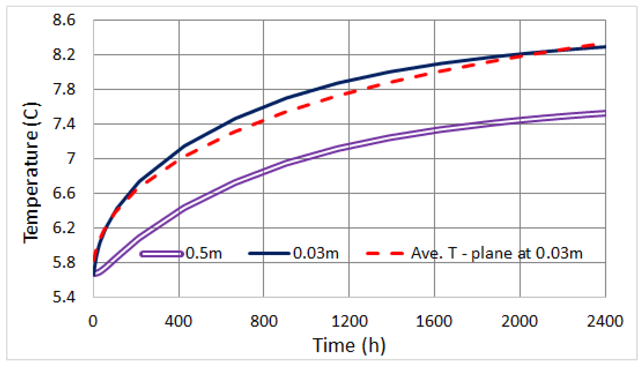
3. Ground Surface Boundary Analysis in COMSOL

After validating the simulation setup, we are now going to use an analogous COMSOL model to study a 2D heat transfer analysis in energy piles with two different boundary conditions at the surface: case (a) single uniform indoor floor, and case (b) outdoor soil/indoor floor slab. The goal of this second case study was assessing the importance of the multiregional boundary condition proposed in [13].

3.1. Method

The calculation at hand consists of a 2D dimensional reduction of the 3D model addressed in Section 2, extended to a multiple piles layout. The 2D COMSOL model in Figure 6 and Figure 7 studies the heat transfer processes occurring between five 15 m-long energy piles, placed under the building, and the surrounding homogeneous soil.
We modelled a 20 m-large floor slab, consisting of two layers: a lower 20 cm-thick EPS layer with k = 0.034 W/mK, ρ = 20 kg/m 3 and c p = 750 kJ/kgK, and an upper 10 cm-thick concrete slab with k = 1.8 W/mK, ρ = 2400 kg/m 3 and c p = 880 kJ/kgK. Each pile was implemented as a 15 m-long concrete grout with diameter 115 mm, surrounding a U-pipe of external diameter 25 mm (their modelling is discussed more into detail in the next Section 3.1). The piles spacing was 4.5 m and they were buried into a soil medium with k = 1.1 W/mK, ρ = 1800 kg/m 3 and c p = 1800 kJ/kgK.
The two cases investigated correspond to two different upper boundary conditions: (a) floor only, set at 20 °C, namely the average annual indoor air temperature of a commercial hall-type building; (b) floor + soil, where the soil extends for 5 m further from each floor edge (see Figure 8). The soil surface was set at T = 5.67 °C, which corresponds to the average annual outdoor air temperature in Southern Finland.
The initial T values were the following: soil layer and grout 5.67 °C, U-pipes 0 °C, upper concrete floor layer 20 °C. The U-pipes were always kept at constant T = 0 °C (corresponds to constant heat pump operation), the floor at 20 °C for both (a) and (b) and the soil surface for case (b) at 5.67 °C. A 2D heat conduction module was used, defined by an equation analogous to (1) that naturally takes into account the mutual thermal interaction of adjacent piles. The mesh was normally sized, tetrahedral and physics-controlled, finer at the soil/pile interface and coarser near the boundaries (Figure 6 and Figure 7), with minimum element size 9 mm and maximum 2 m. The simulation was carried out for 2400 h, with time interval Δ t = 1 h.

Brine Flow Modelling

In standard constructions, the U-pipes inside the energy piles are usually made of high-density polyethylene (HDPE), with a brine fluid (mostly a water/ethanol mixture) flowing inside [53].
Since the simulations here performed are characterized by large geometry and time scales ( Δ t = 1 h and t t o t = 2400 h), it is legitimate to be concerned with the computational problems related to the inclusion of a fluid dynamics module. For the same reasons though, simulating the fluid flow in the pipes should not be necessary, since high-resolution microphysical processes (inducing fluctuations, turbulences and local irregularities in the brine flow and temperature) should not be relevant.
This reasoning seems to find support in the literature: several examples (see e.g., [56,57]) can be found illustrating how models of transient fluid transport inside the tubes would be justified only for much smaller time scales. In particular, Ref. [56] shows that a steady-state, a transient and a semi transient model converge already after ∼3 h.
There are different ways to simplify the implementation of fluid flow, in order to reduce the computational time; for example, in [25,43] the convective heat transfer associated with the fluid flow was simulated by an equivalent solid with the same thermophysical properties of the actual circulation fluid. In order to quantify the error induced by neglecting the fluid flow, we therefore considered the system in Figure 6 only with heat conduction, and modelled the U pipes as made of concrete at constant temperature 0 °C. The surrounding grout was at 5.67 °C at t = 0 , and then subject to heat transfer for 2400 h. On the other hand, we created another simulation based on the exact same setup, but this time with U-pipes made of water that was flowing at 0 °C, with inlet velocity V i n = 0.45 m/s and ignoring the pipe thickness.
The result is plotted in Figure 9, where we compare the average temperature in the soil area surrounding the piles, which is active for heat extraction and is highlighted in Figure 8. One can see that the difference is negligible, confirming our assumption at the beginning of this section that we can safely ignore the fluid flow. We accordingly model the U-pipes as made of concrete with constant T, both in the 2D computations and in the full 3D simulations performed in Section 4 and Section 5. Let us remark however that the above discussion pertains only COMSOL; IDA-ICE, on the other hand, considers the fluid turbulence already by default when computing the convection heat transfer coefficient h.

3.2. Results

In this section we compare and discuss the thermal profiles calculated by COMSOL in the two cases corresponding to two different boundary conditions at surface. To quantify differences in the soil region that is active for heat extraction, we computed the average temperature for the rectangular region highlighted in Figure 8 for both (a) and (b). This extends for 1.5 m from the most external piles on both sides, and for 1m from the piles bottom. Thermal insulation effects at the boundaries (at 0 m, −5 m and 15 m in the plot), which are embedded in COMSOL, should not alter the result as they are washed out by the large amount of soil between boundaries and the region’s edges.
The result is plotted in Figure 10. It is rather evident that, even after so many hours of heat pump operation at full load, no appreciable difference can be discerned, only ∼0.015 °C at the most. We thus conclude that when interested in average temperatures and energy balance, we can freely choose either boundary conditions without compromising our results.

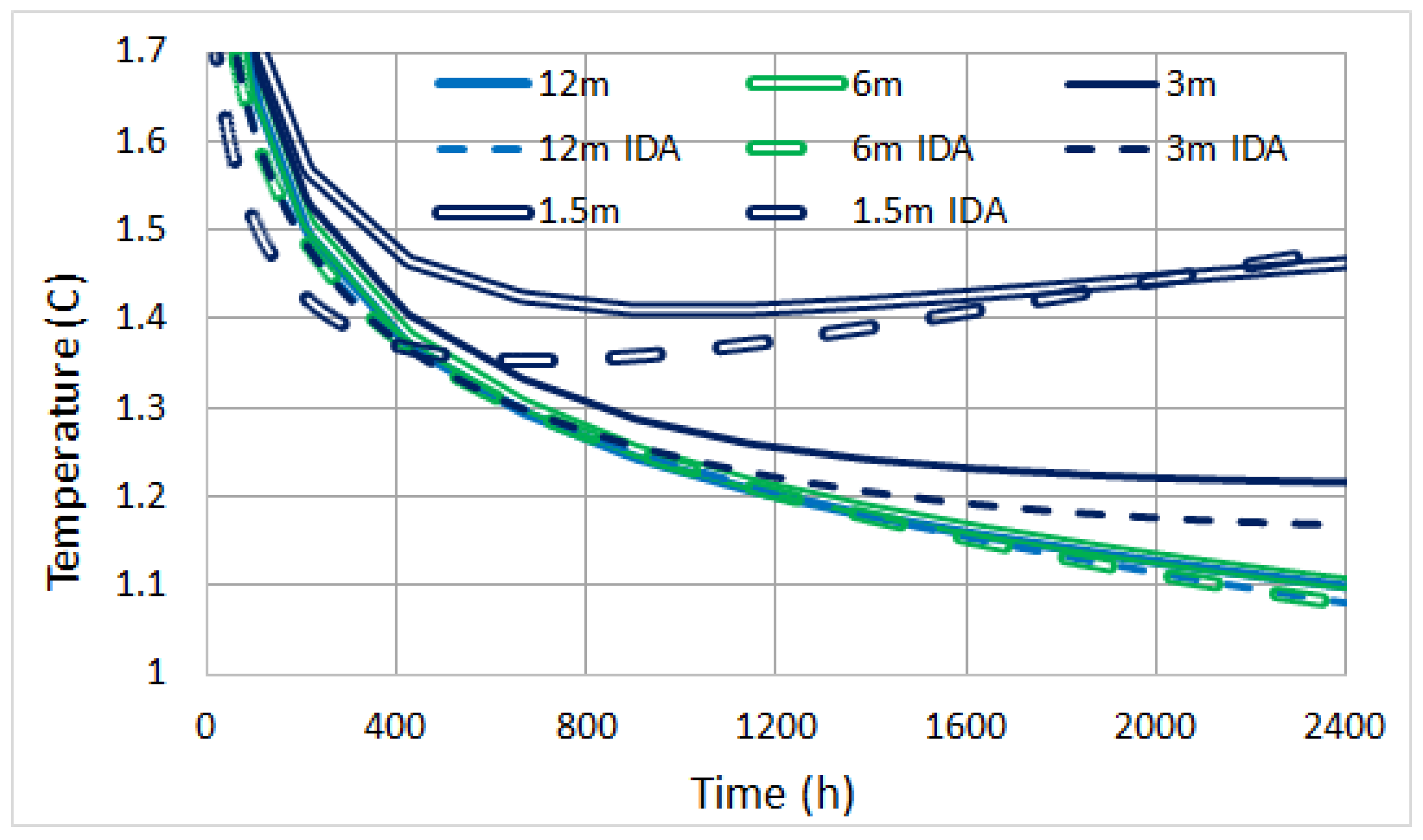
4. IDA-ICE Borehole Model Validation against COMSOL

In this third study we consider a 3D IDA-ICE finite difference borehole model, together with the COMSOL FEM counterpart. The latter is a direct 3D extension of the 2D model discussed in Section 3. Here we compute the outlet temperatures at different depths on the edge of 20 energy piles, which are buried in soil under a multilayer floor. Results from the IDA-ICE model are compared with those obtained from COMSOL, in order to estimate the accuracy of the IDA-ICE calculation.

4.1. Method

A 3D FEM COMSOL extension of the 2D model discussed in Section 3 is here performed, with 20 identical energy piles that are 15 m-long and with 4.5 m spacing; the same geometry is implemented both in COMSOL (Figure 11) and in IDA-ICE, with a 3D finite element (COMSOL) or finite difference (IDA-ICE) borehole model that accounts for the mutual thermal interaction of adjacent piles.
The piles were buried in a 25 m × 25 m × 20 m soil medium (layout listed in Table 3), with the same multilayer floor (concrete slab over an EPS layer) addressed in Section 3 as the upper boundary condition. In IDA-ICE this is set by default because, as remarked earlier, the option to define multiple ground surface boundary regions is not available. Temperature loggers were set on the centre pile #10, on the centre-edge pile #12 and on the edge pile #20, to quantify the impact of surrounding piles on the temperature fields. Temperatures were logged at 1.5 m, 3 m, 6 m and 12 m depth, with loggers located on the pile edge in contact with soil.
In the COMSOL simulation piles, floor and soil were modelled exactly as in Section 3.1, with the same material properties. The concrete floor was kept at 20 °C at all times, and the U-pipes were kept at steady T = 0 °C (corresponding to a constant heat pump operation). In order to decrease the simulation time, no fluid flow was modelled, as explained in Section 3.1; in IDA-ICE instead, the fluid at constant T = 0 °C entered the energy piles at a very high flow rate. Simulations in COMSOL and IDA-ICE ran for 2400 h, with time interval Δ t = 1 h.

4.2. Results

Looking at Figure 12, Figure 13 and Figure 14, one can clearly see that, as expected, only the central pile #10 is slightly colder than the other two. We do not really see a major impact of the specific placement. Furthermore, predictions of COMSOL and IDA-ICE are extremely close, on the average of the order 0.05 °C. Regardless of the software used, the temperature difference is overall very small, accounting for the soil medium and piles temperature homogeneity. Even a very large depth difference shows little discrepancy, e.g., 1.5 m and 12 m give Δ T < 0.4 °C. Specifically, notice how for every pile, the 12 m curves overlap exactly with those at 6 m. Surface effects are indeed strongly hindered by the large thermal mass of the soil medium. Figure 15 also illustrates that, for different boundary conditions at the surface (full floor vs. floor + soil), COMSOL shows a similar Δ T 0.4 °C. This effect is compensated by averaging over the large area that is active for heat extraction, as we discussed in Section 3.
Surface effects should however be relevant for small depths. We thus consider a point in between the central piles, at 0.5 m under the floor, and compare its temperature profile to that of another point right above, very close to the floor, at 3 cm depth. As illustrated in Figure 16, after about 200 h (i.e., after the FEM simulation is stabilised) there is a constant Δ T 0.8 °C. This means that, differently from what we have seen above for points sitting deeper underground, when approaching the surface T differences are relevant and cannot be ignored.
More importantly though, Figure 16 also shows that the integrated average temperature on a plane located at 3 cm under the floor, pictured in Figure 11, always coincides with T as computed at a central point at the same depth. This is a natural consequence of the simulation’s geometrical and physical symmetry, showing that for a similar setup one can use averages instead of point values. This result might be valuable for practitioners and on-site applications.

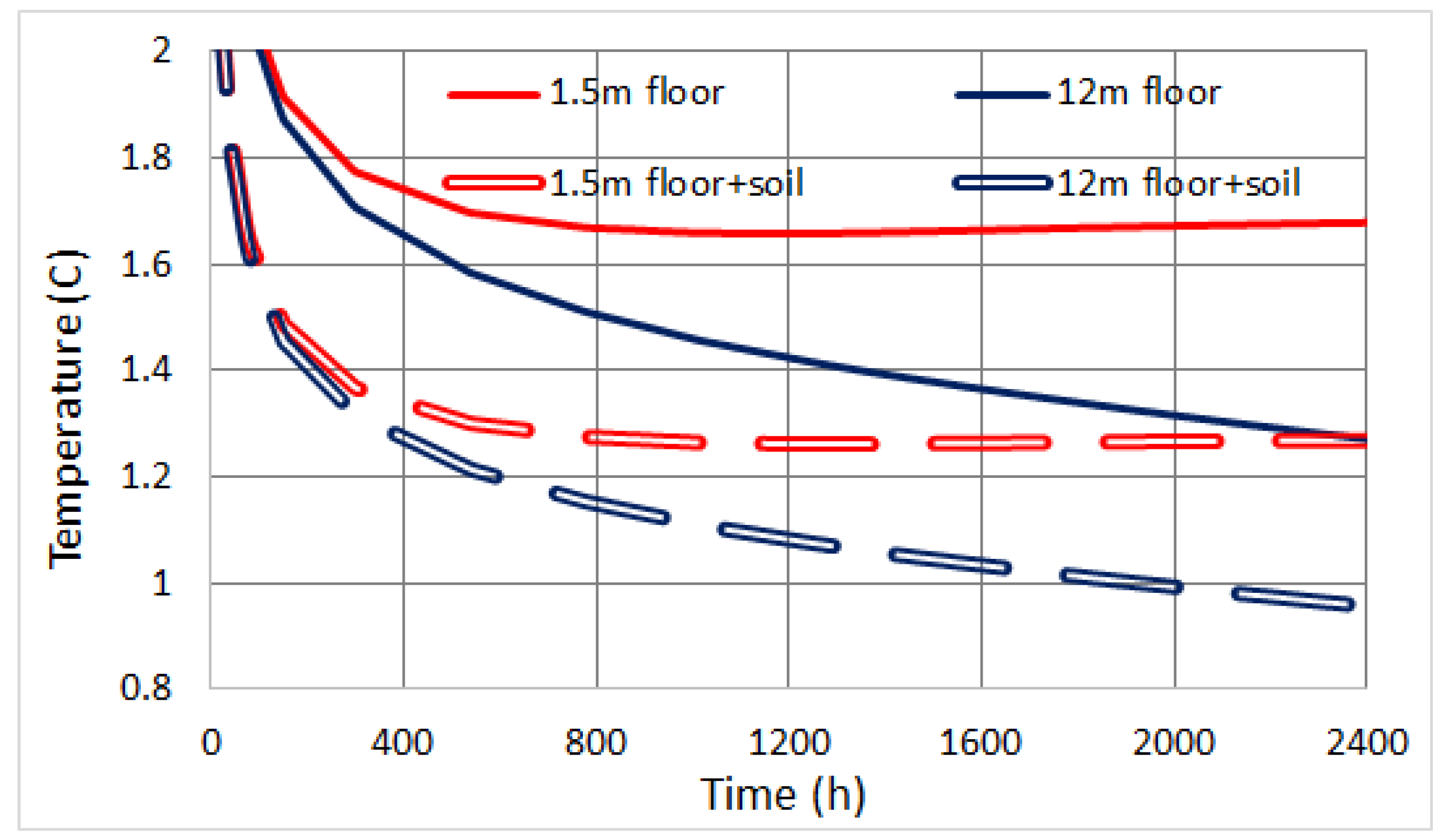
5. Impact of Boundary Conditions on Energy Efficiency Calculations

In this final case, we apply to a 3D COMSOL FEM model the data obtained in [28] by modelling the energy piles with IDA-ICE, in order to calculate the temperature underneath the floor slab (also called “ground surface temperature”). The result is then compared to the rough estimation made in [28] (the “outlet” solution here), and to an analogous IDA-ICE calculation using a new software version updated in November 2017 (the “slab” solution here). We find that the new implementation “slab” shows a remarkable improvement over the "outlet" method in terms of energy consumption assessment.

5.1. Method

Geothermal energy piles with heat pump in a whole building were modelled in IDA-ICE following the design proposed in [28] and addressing the same commercial hall-type building (Figure 17). The total number of energy piles was 192, the initial soil temperature 5.67 °C and the piles were 15 m-long. The soil properties were k = 1.1 W/mK, ρ = 1800 kg/m 3 and c p = 1800 kJ/kgK.
In the present study, we performed an annual IDA-ICE simulation according to this design. We obtained inlet and outlet energy piles temperatures with hourly resolution, which we used to calculate the average energy piles fluid temperature. These were then implemented in COMSOL as boundary conditions, to avoid including a fluid dynamics module for the reasons explained in Section 3.1. Our COMSOL simulation accordingly involves only heat conduction, but uses the IDA-ICE values to increase the precision.
To compute the yearly energy demand for this building, the model was divided into two zones—one with energy piles and one without. The building floor slab above the energy piles accounts for ca. 33% of the total floor slab area. In the original “outlet” approach presented in [28], a variable temperature underneath this surface is roughly estimated as the energy piles outlet temperature, with connection scheme presented in Figure 18. This was necessary since before November 2017 it was not possible for IDA-ICE to calculate the exact ground surface temperature above the piles, which we accomplish instead with the new solution called “slab”.
The annual simulation with hourly resolution performed in COMSOL returned the average ground surface temperature T s beneath the floor slab, then compared against the same T s calculated by the new “slab” borehole model. Finally, we quantify the discrepancy between COMSOL and the two IDA-ICE models “outlet” and “slab” when computing the yearly energy need for the above building.

5.2. Results

Figure 19 compares the COMSOL-calculated ground surface temperature against the two temperatures estimated in IDA-ICE. In the previous IDA-ICE “outlet” approach [28], the results were obtained with an outdated version of the software, where the borehole model uses the energy piles outlet temperature as a rough estimate for the ground surface temperature.
The newer IDA-ICE “slab” estimates use instead the latest version of borehole model, which is now capable of estimating the ground surface temperature. One can observe a significant difference of 5.8 °C between the new and old version over the simulated annual period. Remarkably, the new result of IDA-ICE borehole model differs by only 0.6 °C from COMSOL.
Table 4 shows how improper modelling of the ground surface temperature affects the floor slab heat flux over the energy piles, and accordingly the overall annual heat demand of the building. From the perspective of annual heat flux difference, simply applying the outlet temperature of energy piles as ground surface boundary condition in “outlet” produces a difference in ca. 54%, which induces nearly a 5% overestimation of building annual heating need. In contrast, the new version of borehole model “slab” performs in a very good agreement with COMSOL, within an acceptable heat flux and heating need difference of 0.03% and 0.2% respectively.
The new IDA-ICE implementation of a borehole model is therefore free from previous heating consumption overestimations, providing a reliable tool for investigations of building heating needs.

6. Conclusions

In this paper we have investigated into detail geothermal plants modelling, by comparing different boundary conditions and their impact on numerical studies of heat transfer and energy performance. First we considered the finite element method (FEM) software COMSOL Multiphysics, and validated a 3D model of transient heat transfer against experimental data. We found an excellent agreement, despite uncertainties in the measurements and estimated soil properties.
Next we simulated transient heat transfer in a multi-pile 2D reduction of the previous simulation, and addressed the effect of different upper boundary conditions, namely either (i) a unique floor multilayer at 20 °C or (ii) a floor at 20 °C and soil at ∼6 °C. We found that for practical purposes, the average temperatures and energy balance for a yearly calculation are unaffected by the specific boundary condition. This holds by virtue of extremely small temperature differences in the active heat extraction region: modelling of energy piles can thus be performed using borehole models with variable ground surface temperature, which can be set as the indoor air temperature above the energy piles area. The implementation of multiregional surface boundary conditions proposed in [13] can be accordingly neglected in future studies.
As a side result, we discussed the role of fluid flow modelling inside the pipes. We confirm earlier findings that for the length and time scales of interest, one can safely ignore the fluid flow and model the U-pipes as made of concrete with constant T, both in 2D and 3D simulations.
A third computation was then performed with both COMSOL and IDA-ICE, addressing transient heat transfer for 2400 h. The simulations consisted of a 3D model with 20 energy piles embedded in a soil medium, under a uniform multilayer floor, revealing that temperature predictions of COMSOL and IDA-ICE are extremely close, on the average of the order 0.05 °C. In particular, the piles temperatures are not affected by the specific placement, as they are approximately constant for a given depth. The large thermal mass of piles and medium also provides a very small vertical gradient, e.g., the difference between 1.5 m and 12 m depth gives only Δ T < 0.4 °C. Moreover, for every pile the 12 m curves overlap exactly with those at 6 m.
Figure 15 illustrates a comparable Δ T 0.4 °C also for different boundary conditions at the surface (full floor vs. floor + soil) in COMSOL. This effect is compensated by averaging over the large area that is active for heat extraction, as we discussed in Section 3. However, close to the surface the different boundary conditions (full floor vs. floor + soil) do give a different temperature. Interestingly, we also found that the integrated average T on a horizontal plane at height h is nearly identical to the one at a point laying on it. This result could be useful for practical calculations of energy balance over the same time scale.
Finally, we performed a yearly simulation to assess the heating need of a commercial building employing a geothermal plant. Assuming the COMSOL FEM calculation validated in Section 1 as our benchmark, two IDA-ICE FDM simulations illustrated the impact of different upper boundary conditions on the final energy consumption estimate. We found that in IDA-ICE, adopting the energy piles outlet temperature as a rough estimate for the ground surface temperature overestimates the heat flux in the floor slab by 54% and the heating need by 5%. On the other hand, using the ground surface temperature produced a consistent result with COMSOL, overestimating the heat flux and heating need by only 0.03% and 0.2% respectively.
One might now wonder about the long-term effects of the heat discharge. This has been studied into details in [28] for a heat pump plant with energy piles serving a one storey commercial hall building. Long-term simulations encompassing 20 years of usage showed a consistent reduction in performance of the energy piles regarding heat extraction. It was found indeed that, over the years, the heat extracted from the energy piles exceeds the amount which is loaded during the cooling season. Evidently, this implies a need for thermal storage, at least for the case of commercial hall-type buildings.
In conclusion, this paper provides a through comparison of software widely used in simulations of heating systems adopting borehole and energy piles. In particular, focusing on the role of upper boundary conditions, we showed that multiregional b.c. are fairly equivalent to a single surface with uniform temperature. Moreover, we proved that using the pipes outlet temperature induces a severe overestimation of the heat flux through the heated floor and of the energy demand for the whole building.
All these results are relevant especially for practical purposes, in the development of geothermal energy methods in compliance with international Standards and towards sustainability. In this perspective, they set the foundation for a number of necessary developments and improvements: for instance, longer term simulations (such as 10–20 years) could investigate the effect of a reverse operation mode in summer, for decharging the ground to limit the thermal drift observed in [28]. Other possibilities could be the extension of our methodology to other types of climates, and the assessment of thermomechanical effects on the piles’ structure.

Author Contributions

Conceptualization, A.F., J.F. and J.K.; methodology, A.F. and J.F.; software, A.F. and J.F.; validation, A.F.; investigation, A.F. and J.F.; writing—original draft preparation, A.F. and J.F.; writing—review and editing, A.F.; supervision, J.K.; funding acquisition, J.K.

Funding

The research was supported by the Estonian Research Council with Institutional research funding grant IUT1-15. The authors are also grateful to the Estonian Centre of Excellence in Zero Energy and Resource Efficient Smart Buildings and Districts, ZEBE, grant 2014-2020.4.01.15-0016 funded by the European Regional Development Fund.

Conflicts of Interest

The authors declare no conflict of interest.

Abbreviations

The following abbreviations have been used in this manuscript:
GHEGround Heat Exchangers
FEMFinite Element Method
FDMFinite Difference Method
b.c.Boundary Conditions
Nomenclature
ρ Density [kg/m 3 ]
c p Specific heat at constant pressure [kJ/(kgK)]
TTemperature [°C]
λ Thermal conductivity [W/(mK)]
Δ t Time step [h]

References

  1. European Parliament. Directive 2010/31/EU of the European Parliament and of the Council of 19 May 2010 on the energy performance of buildings. Off. J. Eur. Union 2010, 53, 13–35. [Google Scholar]
  2. Lund, J.W.; Boyd, T.L. Direct utilization of geothermal energy 2015 worldwide review. Geothermics 2016, 60, 66–93. [Google Scholar] [CrossRef]
  3. Agemar, T.; Weber, J.; Moeck, I.S. Assessment and Public Reporting of Geothermal Resources in Germany: Review and Outlook. Energies 2018, 11, 332. [Google Scholar] [CrossRef]
  4. Park, K.S.; Kim, S. Utilising Unused Energy Resources for Sustainable Heating and Cooling System in Buildings: A Case Study of Geothermal Energy and Water Sources in a University. Energies 2018, 11, 1836. [Google Scholar] [CrossRef]
  5. Aydin, M.; Sisman, A. Experimental and computational investigation of multi U-tube boreholes. Appl. Energy 2015, 145, 163–171. [Google Scholar] [CrossRef]
  6. Bose, J.E.; Smith, M.; Spitler, J. Advances in ground source heat pump systems-an international overview. In Proceedings of the 7th IEA Heat Pump Conference, Beijing, China, 19–22 May 2002; Volume 324, pp. 313–324. [Google Scholar]
  7. Spitler, J. Editorial: Ground-Source Heat Pump System Research—Past, Present, and Future. HVAC R Res. 2005, 11, 165–167. [Google Scholar] [CrossRef]
  8. Brandl, H. Energy foundations and other thermo-active ground structures. Geotechnique 2006, 56, 81–122. [Google Scholar] [CrossRef]
  9. Lautkankare, R.; Sarola, V.; Kanerva-Lehto, H. Energy piles in underpinning projects—Through holes in load transfer structures. DFI J. J. Deep Found. Inst. 2014, 8, 3–14. [Google Scholar] [CrossRef]
  10. Faizal, M.; Bouazza, A.; Singh, R.M. Heat transfer enhancement of geothermal energy piles. Renew. Sustain. Energy Rev. 2016, 57, 16–33. [Google Scholar] [CrossRef]
  11. Bourne-Webb, P.; Burlon, S.; Javed, S.; Kuerten, S.; Loveridge, F. Analysis and design methods for energy geostructures. Renew. Sustain. Energy Rev. 2016, 65, 402–419. [Google Scholar] [CrossRef] [Green Version]
  12. Li, M.; Lai, A.C. Review of analytical models for heat transfer by vertical ground heat exchangers (GHEs): A perspective of time and space scales. Appl. Energy 2015, 151, 178–191. [Google Scholar] [CrossRef]
  13. Fadejev, J.; Simson, R.; Kurnitski, J.; Haghighat, F. A review on energy piles design, sizing and modelling. Energy 2017, 122, 390–407. [Google Scholar] [CrossRef]
  14. Ingersoll, L.R.; Zobel, O.J.; Ingersoll, A.C. Heat conduction with engineering, geological and other applications. Q. J. R. Meteorol. Soc. 1955, 81, 647–648. [Google Scholar] [CrossRef]
  15. Goldenberg, H. A problem in radial heat flow. Br. J. Appl. Phys. 1951, 2, 233. [Google Scholar] [CrossRef]
  16. Hu, P.; Zha, J.; Lei, F.; Zhu, N.; Wu, T. A composite cylindrical model and its application in analysis of thermal response and performance for energy pile. Energy Build. 2014, 84, 324–332. [Google Scholar] [CrossRef]
  17. Abdelaziz, S.L.; Ozudogru, T.Y. Selection of the design temperature change for energy piles. Appl. Therm. Eng. 2016, 107, 1036–1045. [Google Scholar] [CrossRef]
  18. Hellström, G. Ground Heat Storage: Thermal Analyses of Duct Storage Systems. Ph.D. Thesis, School of Mathematical Physics, Lund University, Lund, Sweden, 1991. [Google Scholar]
  19. Claesson, J.; Hellström, G. Analytical studies of the influence of regional groundwater flow on the performance of borehole heat exchangers. In Proceedings of the 8th International Conference on Thermal Energy Storage, Terrastock 2000, Stuttgart, Germany, 28 August–1 September 2000; pp. 195–200. [Google Scholar]
  20. Bozis, D.; Papakostas, K.; Kyriakis, N. On the evaluation of design parameters effects on the heat transfer efficiency of energy piles. Energy Build. 2011, 43, 1020–1029. [Google Scholar] [CrossRef]
  21. Rosa, M.D.; Ruiz-Calvo, F.; Corberán, J.M.; Montagud, C.; Tagliafico, L.A. Borehole modelling: A comparison between a steady-state model and a novel dynamic model in a real ON/OFF GSHP operation. J. Phys. Conf. Ser. 2014, 547, 012008. [Google Scholar] [CrossRef]
  22. Kwong Lee, C.; Nam Lam, H. Thermal Response Test Analysis for an Energy Pile in Ground-Source Heat Pump Systems. In Progress in Sustainable Energy Technologies: Generating Renewable Energy; Dincer, I., Midilli, A., Kucuk, H., Eds.; Springer: Cham, Switzerland, 2014; pp. 605–615. [Google Scholar]
  23. Li, Z.; Zheng, M. Development of a numerical model for the simulation of vertical U-tube ground heat exchangers. Appl. Therm. Eng. 2009, 29, 920–924. [Google Scholar] [CrossRef]
  24. Nam, Y.; Ooka, R.; Hwang, S. Development of a numerical model to predict heat exchange rates for a ground-source heat pump system. Energy Build. 2008, 40, 2133–2140. [Google Scholar] [CrossRef]
  25. Lazzari, S.; Priarone, A.; Zanchini, E. Long-term performance of BHE (borehole heat exchanger) fields with negligible groundwater movement. Energy 2010, 35, 4966–4974. [Google Scholar] [CrossRef]
  26. Diersch, H.J.; Bauer, D.; Heidemann, W.; Rühaak, W.; Schätzl, P. Finite element modeling of borehole heat exchanger systems: Part 2. Numerical simulation. Comput. Geosci. 2011, 37, 1136–1147. [Google Scholar] [CrossRef]
  27. Salvalai, G. Implementation and validation of simplified heat pump model in IDA-ICE energy simulation environment. Energy Build. 2012, 49, 132–141. [Google Scholar] [CrossRef]
  28. Fadejev, J.; Kurnitski, J. Geothermal energy piles and boreholes design with heat pump in a whole building simulation software. Energy Build. 2015, 106, 23–34. [Google Scholar] [CrossRef]
  29. Østergaard, D.; Svendsen, S. Space heating with ultra-low-temperature district heating—A case study of four single-family houses from the 1980s. Energy Procedia 2017, 116, 226–235. [Google Scholar] [CrossRef]
  30. Schweiger, G.; Heimrath, R.; Falay, B.; O’Donovan, K.; Nageler, P.; Pertschy, R.; Engel, G.; Streicher, W.; Leusbrock, I. District energy systems: Modelling paradigms and general-purpose tools. Energy 2018, 164, 1326–1340. [Google Scholar] [CrossRef]
  31. Lee, C.; Lam, H. A simplified model of energy pile for ground-source heat pump systems. Energy 2013, 55, 838–845. [Google Scholar] [CrossRef]
  32. Mehrizi, A.A.; Porkhial, S.; Bezyan, B.; Lotfizadeh, H. Energy pile foundation simulation for different configurations of ground source heat exchanger. Int. Commun. Heat Mass Transf. 2016, 70, 105–114. [Google Scholar] [CrossRef]
  33. Xiao, J.; Luo, Z.; Martin, J.R.; Gong, W.; Wang, L. Probabilistic geotechnical analysis of energy piles in granular soils. Eng. Geol. 2016, 209, 119–127. [Google Scholar] [CrossRef]
  34. Pryor, R.W. Multiphysics Modeling Using COMSOL: A First Principles Approach, 1st ed.; Jones and Bartlett Publishers, Inc.: Burlington, MA, USA, 2009. [Google Scholar]
  35. Dupray, F.; Laloui, L.; Kazangba, A. Numerical analysis of seasonal heat storage in an energy pile foundation. Comput. Geotech. 2014, 55, 67–77. [Google Scholar] [CrossRef]
  36. Diersch, H.J.; Bauer, D.; Heidemann, W.; Rühaak, W.; Schätzl, P. Finite element modeling of borehole heat exchanger systems: Part 1. Fundamentals. Comput. Geosci. 2011, 37, 1122–1135. [Google Scholar] [CrossRef]
  37. Park, H.; Lee, S.R.; Yoon, S.; Choi, J.C. Evaluation of thermal response and performance of PHC energy pile: Field experiments and numerical simulation. Appl. Energy 2013, 103, 12–24. [Google Scholar] [CrossRef]
  38. Cecinato, F.; Loveridge, F.A. Influences on the thermal efficiency of energy piles. Energy 2015, 82, 1021–1033. [Google Scholar] [CrossRef] [Green Version]
  39. Ng, C.; Ma, Q.; Gunawan, A. Horizontal stress change of energy piles subjected to thermal cycles in sand. Comput. Geotech. 2016, 78, 54–61. [Google Scholar] [CrossRef]
  40. Go, G.H.; Lee, S.R.; Yoon, S.; byul Kang, H. Design of spiral coil PHC energy pile considering effective borehole thermal resistance and groundwater advection effects. Appl. Energy 2014, 125, 165–178. [Google Scholar] [CrossRef]
  41. Loveridge, F.; Powrie, W. 2D thermal resistance of pile heat exchangers. Geothermics 2014, 50, 122–135. [Google Scholar] [CrossRef] [Green Version]
  42. Alberdi-Pagola, M.; Poulsen, S.E.; Jensen, R.L.; Madsen, S. Thermal design method for multiple precast energy piles. Geothermics 2019, 78, 201–210. [Google Scholar] [CrossRef]
  43. Batini, N.; Loria, A.F.R.; Conti, P.; Testi, D.; Grassi, W.; Laloui, L. Energy and geotechnical behaviour of energy piles for different design solutions. Appl. Therm. Eng. 2015, 86, 199–213. [Google Scholar] [CrossRef]
  44. Caulk, R.; Ghazanfari, E.; McCartney, J.S. Parameterization of a calibrated geothermal energy pile model. Geomech. Energy Environ. 2016, 5, 1–15. [Google Scholar] [CrossRef]
  45. Loria, A.F.R.; Vadrot, A.; Laloui, L. Analysis of the vertical displacement of energy pile groups. Geomech. Energy Environ. 2018, 16, 1–14. [Google Scholar] [CrossRef]
  46. Li, M.; Lai, A.C. Heat-source solutions to heat conduction in anisotropic media with application to pile and borehole ground heat exchangers. Appl. Energy 2012, 96, 451–458. [Google Scholar] [CrossRef]
  47. Park, S.; Lee, D.; Lee, S.; Chauchois, A.; Choi, H. Experimental and numerical analysis on thermal performance of large-diameter cast-in-place energy pile constructed in soft ground. Energy 2017, 118, 297–311. [Google Scholar] [CrossRef]
  48. McCartney, J.S.; Murphy, K.D. Investigation of potential dragdown/uplift effects on energy piles. Geomech. Energy Environ. 2017, 10, 21–28. [Google Scholar] [CrossRef]
  49. Sung, C.; Park, S.; Lee, S.; Oh, K.; Choi, H. Thermo-mechanical behavior of cast-in-place energy piles. Energy 2018, 161, 920–938. [Google Scholar] [CrossRef]
  50. Singh, R.; Bouazza, A.; Wang, B. Near-field ground thermal response to heating of a geothermal energy pile: Observations from a field test. Soils Found. 2015, 55, 1412–1426. [Google Scholar] [CrossRef] [Green Version]
  51. Suryatriyastuti, M.; Mroueh, H.; Burlon, S. Understanding the temperature-induced mechanical behaviour of energy pile foundations. Renew. Sustain. Energy Rev. 2012, 16, 3344–3354. [Google Scholar] [CrossRef]
  52. Eguaras-Martínez, M.; Vidaurre-Arbizu, M.; Martín-Gómez, C. Simulation and evaluation of Building Information Modeling in a real pilot site. Appl. Energy 2014, 114, 475–484. [Google Scholar] [CrossRef] [Green Version]
  53. Uotinen, V.M.; Repo, T.; Vesamäki, H. Energy piles—Ground energy system integrated to the steel foundation piles. In Proceedings of the 16th Nordic Geotechnical Meeting (NGM 2012), Copenhagen, Denmark, 9–12 May 2012; pp. 837–844. [Google Scholar]
  54. Jõeleht, A.; Kukkonen, I.T. Physical properties of Vendian to Devonian sedimentary rocks in Estonia. GFF 2002, 124, 65–72. [Google Scholar] [CrossRef]
  55. Kukkonen, I.; Lindberg, A. Thermal Properties of Rocks at the Investigation Sites: Measured and Calculated Thermal Conductivity, Specific Heat Capacity and Thermal Diffusivity; Working Report; Ilmo Kukkonen Antero Lindberg: Helsinki, Finland, 1998. [Google Scholar]
  56. Bauer, D.; Heidemann, W.; Diersch, H.J. Transient 3D analysis of borehole heat exchanger modeling. Geothermics 2011, 40, 250–260. [Google Scholar] [CrossRef]
  57. Al-Khoury, R.; Kölbel, T.; Schramedei, R. Efficient numerical modeling of borehole heat exchangers. Comput. Geosci. 2010, 36, 1301–1315. [Google Scholar] [CrossRef]
Figure 1. Energy piles (circles) and monitoring layout (undisturbed T monitored at the isolated triangle) [53].
Energies 12 00770 g001
Figure 2. Sketch of sensor placement in soil, on the surface of each pile.
Energies 12 00770 g002
Figure 3. COMSOL simulation for the Innova office building reference pile. (Left) the pile geometry (sensor T31 in red). (Right) the result after t = 4800 h.
Energies 12 00770 g003
Figure 4. Measured (dashed) vs. COMSOL simulated (solid) temperatures for a single pile, sensors at 0.5 m and 4.5 m. Surface temperature in small dashes.
Energies 12 00770 g004
Figure 5. Data (dashed) vs. COMSOL T (solid) for sensors at 4.5 m, 10.5 m and 16.5 m depth.
Energies 12 00770 g005
Figure 6. COMSOL mesh for case (a), only floor.
Energies 12 00770 g006
Figure 7. COMSOL mesh for case (b), floor and soil.
Energies 12 00770 g007
Figure 8. 2D COMSOL result after 2400 hrs for (left) (a) only floor and (right) (b) floor + soil as upper boundary.
Energies 12 00770 g008
Figure 9. Average temperature in the highlighted area of Figure 8 with fluid flow modelling (solid) compared with no fluid modelling (dashed).
Energies 12 00770 g009
Figure 10. Average temperature in the highlighted slab portion, (a) floor (dashed) vs. (b) floor + soil (solid). T [°C] values for the last point in bold.
Energies 12 00770 g010
Figure 11. Floor slab with 20 energy piles in COMSOL. Data point at 9 m shown as a red dot.
Energies 12 00770 g011
Figure 12. Pile #10.
Energies 12 00770 g012
Figure 13. Pile #12.
Energies 12 00770 g013
Figure 14. Pile #20.
Energies 12 00770 g014
Figure 15. COMSOL comparison of different boundary conditions.
Energies 12 00770 g015
Figure 16. Temperature at mid points and on a plane parallel to the floor.
Energies 12 00770 g016
Figure 17. Building model with a separated zone (centre) above energy piles modelled in IDA-ICE.
Energies 12 00770 g017
Figure 18. Connection scheme for “slab” (left) and “outlet” (right) IDA-ICE borehole models.
Energies 12 00770 g018
Figure 19. Estimated IDA-ICE ground surface temperature vs. calculated in COMSOL.
Energies 12 00770 g019
Table 1. Temperature sensors location for the reference energy pile [53].
Temperature SensorDepth, m
Ground surface0
Pile top−0.5
T28−0.5
T29−2.5
T30−4.5
T31−6.5
T32−8.5
T33−10.5
T34−12.5
T35−14.5
T36−16.5
Table 2. Soil layer properties for the single pile simulation [53].
Layer nrDepth, m ρ , t/m 3 c p , kJ/kgK λ , W/mK
13.731.41.80.87
25.671.721.821.24
35.841.661.781.08
46.51.801.711.25
56.671.831.721.39
66.841.911.571.42
712.92.031.401.89
812.912.011.391.81
915.902.062.321.92
1015.912.052.331.91
11191.992.391.53
1219.011.952.411.5
1323.32.282.102.52
1426.72.212.162.44
Table 3. Spatial arrangement (view from above) of the energy piles for both IDA-ICE and COMSOL.
17181920
13141516
9101112
5678
1234
Table 4. Validation results for the IDA-ICE estimated ground surface temperature.
CaseFloor Slab Heat Flux, kWh/aHeating Need, kWh/aHeat Flux, % DifferenceHeating Need, % Difference
COMSOL24066142900--
IDA-ICE slab240731425800.03%0.2%
IDA-ICE outlet3712715019654%5%

