Evaluation Study of Potential Use of Advanced Conductors in Transmission Line Projects †

College of Engineering and Technology, American University of the Middle East, Kuwait city 15453, Kuwait
†
This present study is an extension of the paper “Potential Application of the Advanced Conductors in a Transmission Line Project,” presented to 2018 IEEE International Conference on Environment and Electrical Engineering and 2018 IEEE Industrial and Commercial Power Systems Europe (EEEIC / I&CPS Europe), Palermo, Italy, 12–15 June 2018, and published in Conference Proceedings (DOI:10.1109/EEEIC.2018.8493858).
Energies 2019, 12(5), 822; https://doi.org/10.3390/en12050822
Submission received: 14 January 2019
/
Revised: 23 February 2019
/
Accepted: 25 February 2019
/
Published: 1 March 2019
(This article belongs to the Special Issue Selected Papers from EEEIC 2018—18th International Conference on Environment and Electrical Engineering)
Abstract
:Transmission networks recently faced new technical and economic challenges. The direct use of advanced technologies and modern methods could solve these issues. This paper discusses the potential application of straightforward technology such as high-temperature low-sag conductors (HTLScs) as an additional measure for the protection and effective operation of overhead power lines. An evaluation was conducted to determine an approach for selecting the cross-sectional area and type of conductor with respect to a fault current limitation. It showed the potential benefits of using HTLScs based on an assessment of the throughput capacity and up-front capital costs. A case study considered two scenarios: the construction of a new power line and reconductoring of the existing one. The data for a real project with two overhead power lines were used. The obtained results are analyzed and discussed in detail in this paper.
1. Introduction
The integration of fluctuating renewables, load growth, and aging of the current network are the major drivers for the development of the electricity grid through 2030. The existing generation capacity will be replaced by a new one (located differently and farther from load centers), which will lead to the transformation of the generation infrastructure. Moreover, the interconnection capacity is expected to be increased because of the development of wind and solar generation. The grid backbone should also be enhanced for cross-border trading [1,2,3]. For instance, “an overall increase of interconnection capacity by 40% up to 2020 will be required, with further integration after this point” [4] (pp. 14–15). Therefore, high-voltage transmission networks will face challenges. Adaptation alternatives for such scenarios should be provided with the implementation of new technologies. As a result, critical issues related to both the existing and planned grid infrastructure will be raised.
The grid architecture should be considered a priority issue. Because the expansion of the transmission network will be required, there are two main alternatives: the technical reinforcement of the existing grid (voltage upgrade, reconductoring, etc.) or the construction of new transmission lines (TLs) [5]. This is a complex process, especially for new power-line construction, because of the different restrictions such as regulatory frameworks, environmental issues, difficult terrain and weather, and commercial problems [6,7].
The design of a TL usually involves optimization to minimize the capital costs by considering the thermal, mechanical, electrical, and environmental constraints [8,9,10]. Moreover, the problem formulation could consider the minimization of the payback time of the power line [11,12,13], as well as a life-cycle costing [14].
The conductor plays an important role in the overhead power line (OHL) design, and it is one of the major components of the up-front capital costs of the TL because of the technical possibility of providing the throughput capacity of the power line with respect to the prospective load requirements. Appropriate choices for the cross-sectional area of the conductor and its type will ensure lower losses, higher loading, lower greenhouse emissions, higher reliability, and lower investments of the OHL projects in terms of tower design requirements.
In practice, the selection of the optimum cross-sectional area and type of conductor is a difficult task because of the broad set of parameters, which are seldom known. Studies devoted to the optimization problem of minimizing the capital costs of a TL with respect to the selection of the optimum cross-sectional area of the conductor applied deterministic [15,16] and stochastic methods. For instance, the proposed stochastic approach to selecting the conductor cross-section, which takes into account random variables such as the power line load, electricity price, and ambient temperature, was presented in References [17,18,19]; the method of selecting the conductor and tower configuration from an overall system point of view was considered in Reference [20]; and the methodology for selecting both bare wire conductors and ground wires, their spatial arrangement, and the topology of the tower for a project with compact overhead transmission lines with multiple circuits was presented in Reference [21].
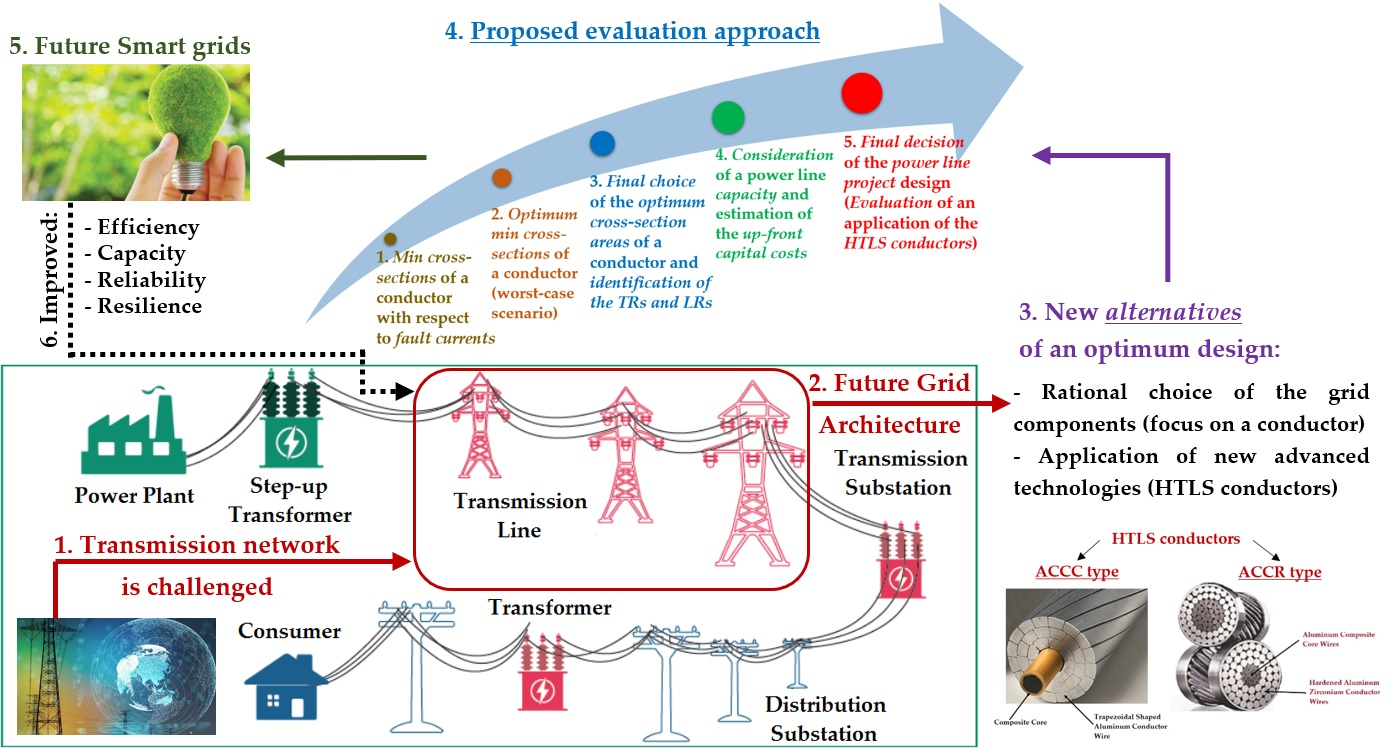
Many different types of conductors were used since OHLs were first installed. The major part of an existing transmission network already uses conventional conductors—the aluminum conductor steel-reinforced (ACSR) family of conductors [22]. Nevertheless, in recent years, the commonly recognized and applied straightforward technology known as high-temperature low-sag conductors (HTLScs) became an attractive method for increasing the thermal rating of a transmission line. ACSR conductors are known to be able to withstand a continuous temperature of 70–80 °C under normal operating conditions, and up to 100 °C without any sign of deformation in the case of emergency, but for only a short duration. However, HTLScs are capable of operating continuously at high temperatures of up to 150–250 °C with less thermal elongation (low sag) than ACSR conductors [23]. These advanced conductors effectively help address power sector challenges by providing improved grid efficiency, current carrying capacity, reliability, and resilience.
Moreover, another aspect to consider when selecting a new type of conductor is the ease of installation in terms of joint points and their corresponding long-term reliability. Because HTLScs can operate at high temperatures, it is necessary to ensure that their accessories do not deform under a condition of 150 °C or above. Because these advanced conductors have physical dimensions that are almost identical to those of the ACSR family of conductors, it could be stated that the same conductor accessories could be safely used up to a continuous temperature of 150 °C without any deformation, but with slight modifications in the case of need (an existing TL reconstruction). This was subject to further studies related to monitoring and testing the conductors’ accessories (including joints) under different OHL operating conditions, for instance, in References [24,25]. Such a possibility will extend the existing manufacturers’ market by increasing the availability of conductor accessories upon specific needs. If a TL conductor operates at temperatures above 150 °C, one of the solutions is to ensure higher-temperature tests for the standardization of accessories such as clamps/connectors. If the mechanical strength is examined, the same material could be used for the clamp as for the conductor (the OHL design requires reconsideration).
Moreover, the installation process for advanced conductors should be predetermined based on several national and international organizations that develop manufacturing standards, operating rules, design guidelines, and installation procedures, which may or may not be accepted or adapted in a particular region [26,27].
There were numerous studies related to the feasibility of using HTLScs in terms of thermal and mechanical restrictions, which were presented in papers such as References [28,29,30,31,32,33]. However, none of them considered the potential application of such advanced conductors as an additional measure for the preliminary increased protection of a TL with respect to the consideration of short-circuit currents.
The main contribution of this paper is the selection of an optimum cross-sectional area and type for the conductor with respect to the fault current limitation, with a further feasibility study of the application of such advanced conductors. The estimated short-circuit currents were taken into account based on the particular design requirements of the TL project. One of the benefits of a preliminary consideration of the fault current limitation is the improvement of the OHL operation reliability by decreasing the potential fault risk due to the lightning side strokes and overloads. Direct strokes to a TL are known to be infrequent in occurrence compared to side strokes. Studies related to lightning phenomena and prevention measures for an OHL were presented in References [34,35,36]. Furthermore, a short-circuit performance test was conducted in terms of the thermal and mechanical performance of the HTLScs in Reference [37] (p. 10-1), which found that “there is no reason to suspect that these conductor systems are unreliable in the short run (up to five years)”. The impact of short-circuit events on the aluminum conductor composite core (ACCC) were also briefly explained in Reference [26] (p. 103), which stated that the “ACCC conductor’s core is much less thermally conductive than aluminum or steel”.
This study had two main objectives: (1) determining the optimum cross-sectional area of the conductor in terms of the fault current limitation, and (2) evaluating the use of HTLSc types in terms of the OHL capacity and up-front capital costs. This study was based on two scenarios: (1) the construction of a new OHL, and (2) reconstruction of the existing TL (reconductoring with the advanced conductors) for two examined 110 kV power lines.
The rest of the paper is organized as follows: Section 2 shows the general data of the two examined OHLs. Section 3 deals with the proposed evaluation approach applied to a particular TL project. Section 4 reviews the computations results for the optimum cross-sectional area of a conductor with respect to the fault current limitation, as well as the identification of temperature regions and length regions. Section 5 presents and analyzes the obtained results of the HTLSc application in terms of the TL throughput capacity and total up-front capital costs by considering the final choice for the optimum cross-sectional area of the conductor and its type. Section 6 provides a discussion related to the obtained results and presents the main research conclusions.
2. Design of Transmission Line
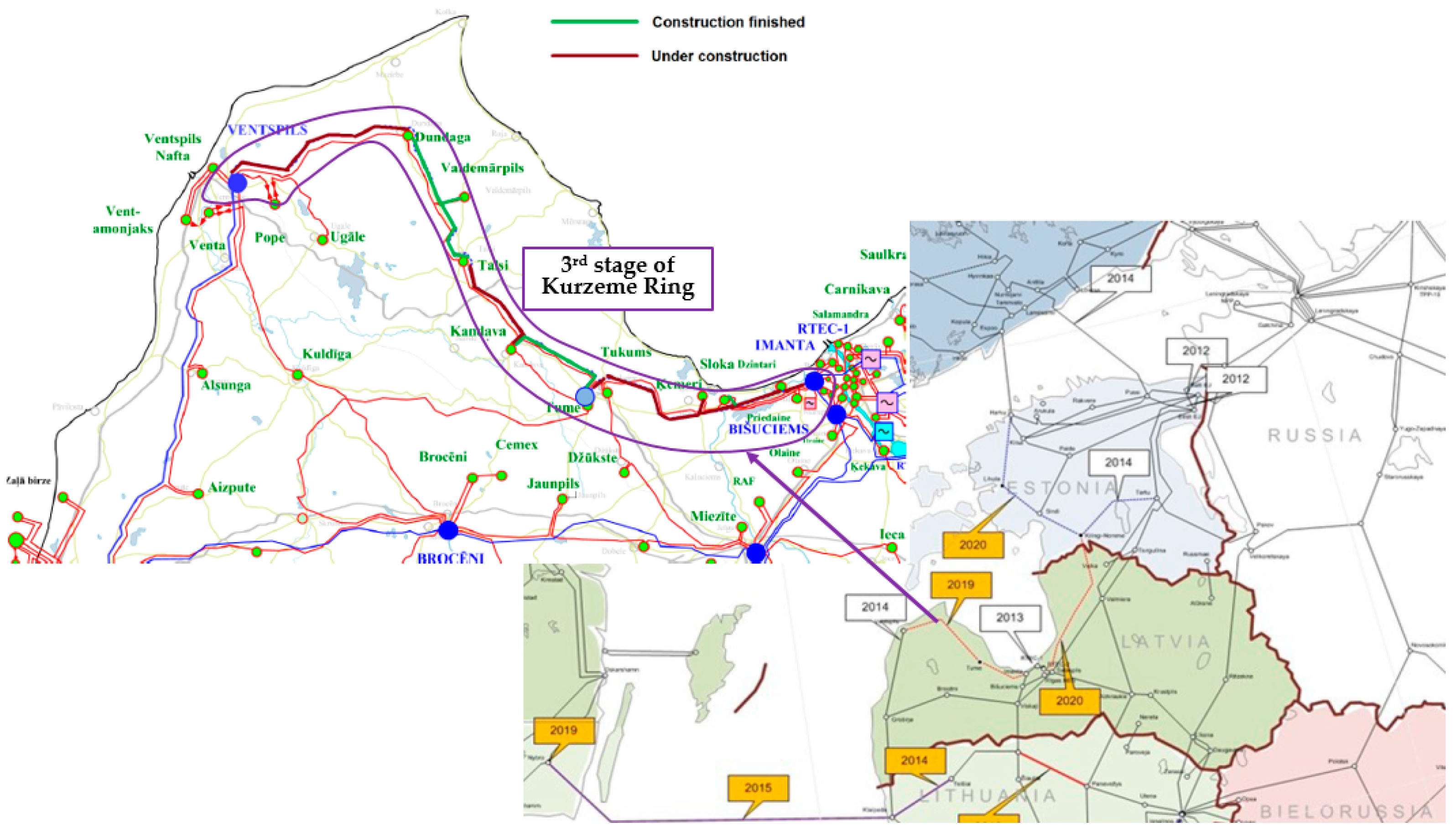
The design of the TL was based on the construction of two new 110 kV OHLs. In particular, “OHL No.1” connects “Substation A” and “Substation B” (total length of 30 km), and “OHL No.2” connects “Substation C” and “Substation B” (total length of 17 km). Thus, “Substation B” is a common substation. The abovementioned 110 kV power lines are a part of the third stage of Latvia’s Kurzeme Ring transmission network [38].
The third stage of the project involves the completion of the TL Ventspils–Tume–Imanta section of the Kurzeme Ring by 2019, thus creating a solid basis for stable and reliable electricity supply in the Baltic region and beyond. The project is part of the Baltic Energy Market Interconnection Plan (BEMIP) and is included in a shortlist as a Project of Common Interest [39]. Figure 1 presents the location of the Kurzeme Ring transmission network in a general overview.
The general requirements adapted for both alternatives (planning a new TL and reconductoring the existing OHL) of the assessed OHLs are as follows:
- The required throughput capacity is 600 A for a single circuit.
- The following climatic conditions in the TL route area are assumed: sun radiation, 850 W/m2; ambient temperature, +35 °C; wind velocity, 0.6 m/s, wind angle, 90°; elevation above sea level, 25 m (average value of the lowest conductor phase); emissivity factor, 0.5; absorptivity factor, 0.8; and load factor, 90%. Moreover, there are issues with the environmental conditions, such as conductor icing (galloping result), which can also impact the conductor selection. These are related to the mechanical limitation of the TL design in the particular areas. There were studies that considered the abovementioned issue, such as References [40,41,42].
The modern integrated OHL design software can be applied when selecting the parameters of the TL, such as the tower and insulator types, and additional line fittings [43].
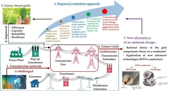
3. Proposed Evaluation Approach
The evaluation approach consists of the following steps:
- (1)
- The required minimum cross-sectional area of a conductor must be calculated with respect to the fault current limitation. Calculations take into consideration the initial temperature of the advanced conductor using 11 temperature points starting from 150 °C to 50 °C, with 10 °C differences between points. Three estimated short-circuit currents, including the phase-to-ground short-circuit (Isc(1)), three-phase short-circuit (Isc(3)), and three times the zero-sequence current (3I0(1,1)) are taken as a basis for further computations of the cross-sectional areas of the conductor. The consideration of the abovementioned short-circuit currents represents the assumed thermal limitation of the conductor (the worst case), and it should be interrupted in less than 5 s (triggering distance protection) [44].
- (2)
- The required minimum cross-sectional area of a conductor must be identified with respect to the maximum short-circuit currents among the three presented and according to each initial conductor temperature. The worst-case scenario is considered (the necessity of a larger cross-section).
- (3)
- The common required minimum conductor cross-sectional areas must be selected with respect to the maximum short-circuit currents and with respect to each initial conductor temperature by revealing overlap regions.
- (4)
- Particular temperature regions (TR), as well as length regions (LR), must be set for the examined power line. The final choice is based on the common required minimum conductor cross-sectional area within the specified overlap regions.
- (5)
- The TL capacity must be estimated with respect to the specific design requirements of the OHL, as well as the up-front capital costs for both applied scenarios.
- (6)
- The obtained computation results for the up-front capital costs and the capacity of the TL must be evaluated with respect to the previously selected cross-sectional area of the conductor and its type for each examined temperature region (TR) and length region (LR).
The obtained results are further considered in the following steps of the above-explained approach in order to reveal and discuss the main outcomes of the proposed research.
4. Choice of Cross-Sectional Area of Conductor with Regard to Fault Current Limitation
4.1. Data on Short-Circuit Currents
The computation of the required minimum cross-sectional area of a conductor of the examined 110 kV OHLs was based on the three estimated short-circuit currents, namely the phase-to-ground short-circuit (Isc(1)), three-phase short-circuit (Isc(3)), and three times the zero-sequence current (3I0(1,1)).
Distance protection is the most common protection principle for OHLs against all types of faults. It is reliable, fast, and able to provide near and far reservation of protection for adjacent objects. More details related to distance protection can be found in References [45,46].
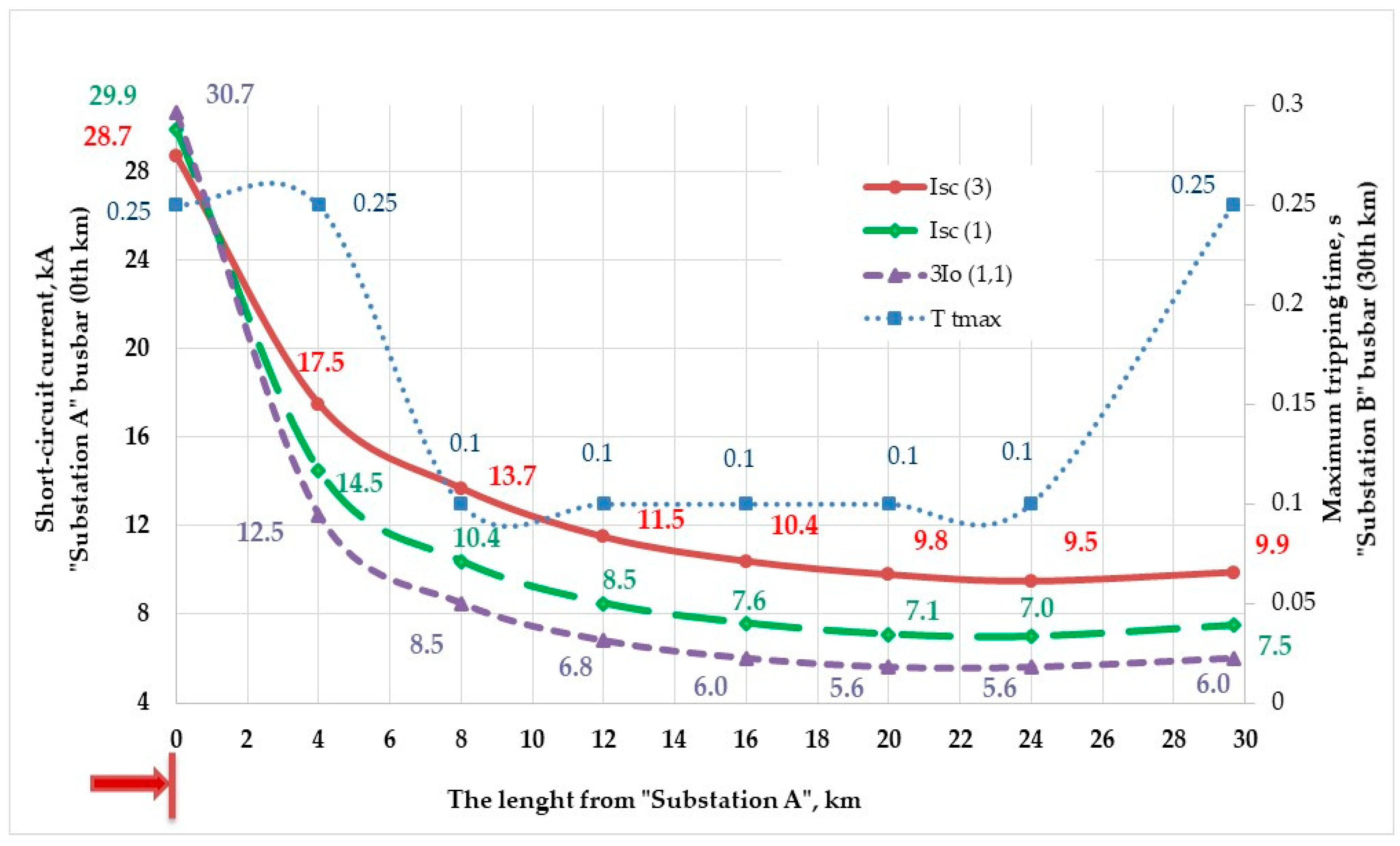
The computations of the short-circuit currents were performed based on the project requirements. The particular approach states that one end of the OHL has a circuit breaker failure; therefore, the TL is without distance protection and without a remote-control communication channel. The short-circuit currents and tripping times were identified for the worst-case scenario based on the maximum “fault current squared multiplied by maximum tripping time (Ttmax)” criteria. The obtained results for the short-circuit currents of “Substation A” and “Substation B” are presented below.
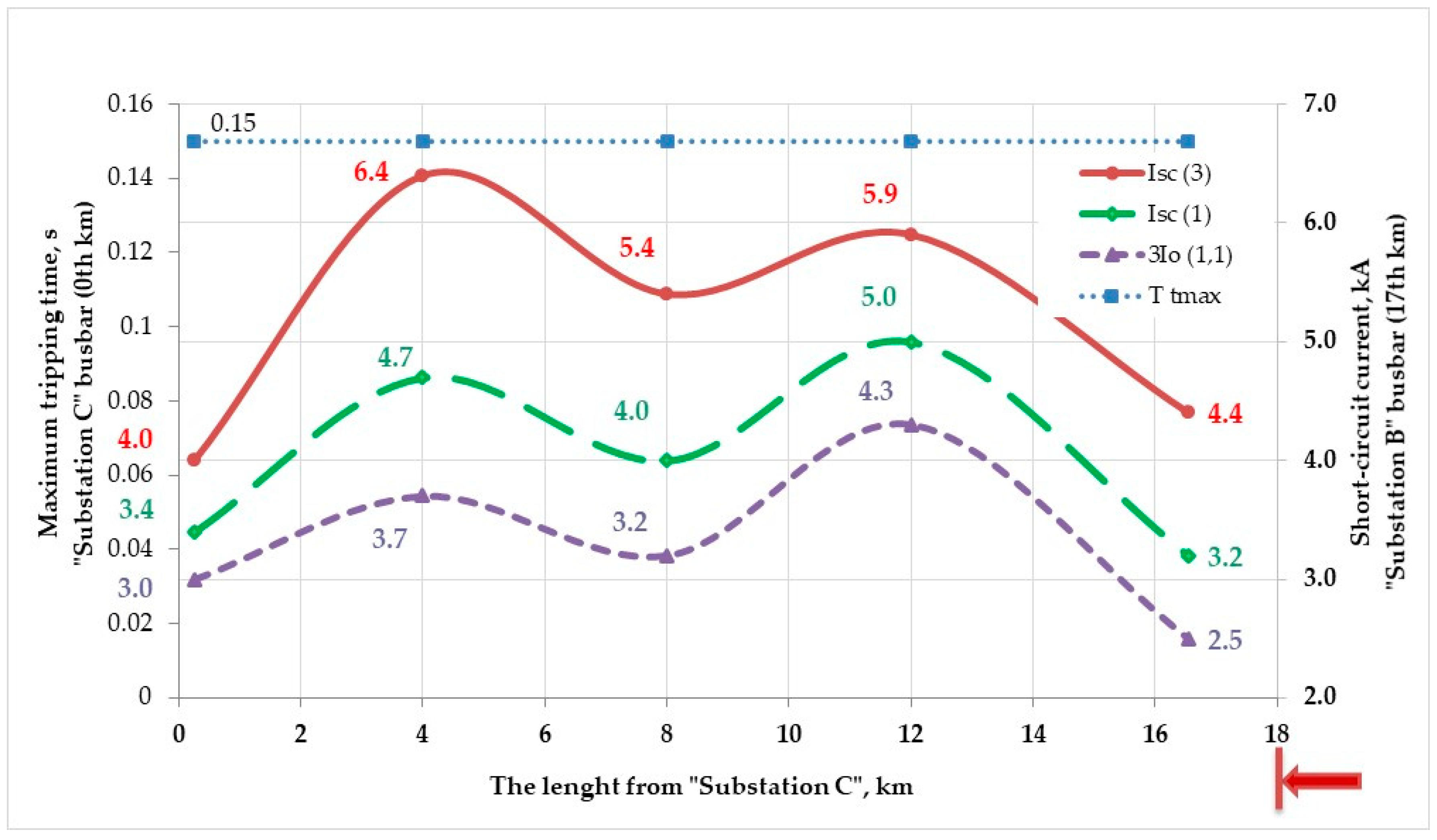
The results obtained for “OHL No.1”, which connects “Substation A” and “Substation B” (total length of 30 km) are presented in Figure 2 and Figure 3. The difference between these two representations is that Figure 2 shows the computations that were performed from “Substation A” toward “Substation B”, while Figure 3 considers the opposite direction, from “Substation B” toward “Substation A”. The same concept is followed for “OHL No.2”, which connects “Substation C” and “Substation B”, where the total length was 17 km (see Figure 4 and Figure 5).
The results of the comparison between the short-circuit currents of the two OHLs are as follows:
- (a)
- “OHL No.1” had very high values for almost all short-circuit current types for the direction considered in Figure 2 (from “Substation A” toward “Substation B”) compared to the other direction in Figure 3. For example, the busbar of “Substation B” of “OHL No.1” (30th km) had 9.9 kA of Isc(3), followed by 7.5 kA of Isc(1), and 6.0 kA of 3I0(1,1). In addition, the maximum value of 3I0(1,1) was equal to 30.7 kA. However, the busbar of “Substation B” for the same “OHL No.1” in the other direction had 4.7 kA of Isc(3), 3.4 kA of Isc(1), and 2.7 kA of 3I0(1,1), and, in this case, Isc(3) had a maximum value of 12 kA.
- (b)
- For “OHL No.2”, when the busbar of “Substation B” was considered, almost the same values of short-circuit currents were observed compared to “OHL No.1” in both directions (see Figure 4 and Figure 5), but the maximum values differed. For instance, in the direction from “Substation C” toward “Substation B” in Figure 4, the maximum value of Isc(3) was equal to 10.3 kA, whereas, in the other direction (see Figure 5), it was 6.4 kA.
- (c)
- The fault current values changed depending on the position of the fault along the TL. The results show that, near the substation busbar (the extremity of the power line), the short-circuit currents were rather high, and the supply circuit was unbalanced compared to these values in the middle of the power line, when the supply circuit was practically balanced. The estimated short-circuit currents for “OHL No.1” especially justify these results. However, the obtained results for “OHL No.2” demonstrate a more balanced supply circuit along the whole length of the power line (the total length of “OHL No.2” was shorter than that of “OHL No.1”).
- (d)
- The results show that, basically, the worst case occurs when the three-phase short-circuit current appears (Isc(3); higher short-circuit current values), for both OHLs. At other times, the worst case occurs for three times the zero-sequence short-circuit current (3I0(1,1)), specifically for “OHL No.1” near the busbar of “Substation A” (up to the fourth km). However, practical TL operation shows that 3I0(1,1) rarely appears compared to a phase-to-ground short-circuit current (Isc(1)).
4.2. Calculations of Required Minimum Cross-Sectional Area of Conductor with Respect to Each Examined Short-Circuit Current
For fault currents that are interrupted in less than 5 s, the minimum required cross-sectional area of a conductor was calculated according to the method and procedure given in Reference [44]. It is worth noting that the concept explained in the proposed approach (see Section 3 on p. 4) adapting this calculation was a slight modification of the approach presentation for the purpose of the computations of the cross-sectional area of the conductor (originally, such a method was used for a selection of the earthing conductor [44]).
In this way, the final computation of the minimum required cross-sectional area of a conductor was calculated as follows:
where
- S
- is the cross-sectional area in mm2;
- I1
- I2
- K
- is a constant in As1/2/mm2 that depends on the material of the current-carrying component, which, for aluminum, is taken to be 148 As1/2/mm2;
- β
- is the reciprocal in °C of the temperature coefficient of the resistance of the current-carrying component at 0 °C, which, for aluminum, is taken to be 228 °C;
- θf
- is the final temperature in °C, which is taken to be 175 °C because of the electrical strength limitation of the aluminum material (with some reserve in terms of reliability);
- θi
- is the initial temperature in °C, where 11 temperature points were here considered from 150 °C to 50 °C with 10 °C differences between points.
The computations of the required minimum cross-sectional area of a conductor were based on each type of estimated short-circuit current. The results are presented below (see Table 1 for “OHL No.1” and Table 2 for “OHL No.2”).
The analysis confirmed that higher cross-sectional areas were calculated for the higher short-circuit currents for both OHLs. A larger cross-sectional area should be applied close to the busbar of any of the considered substations.
The following conclusions can be derived from the results:
- (a)
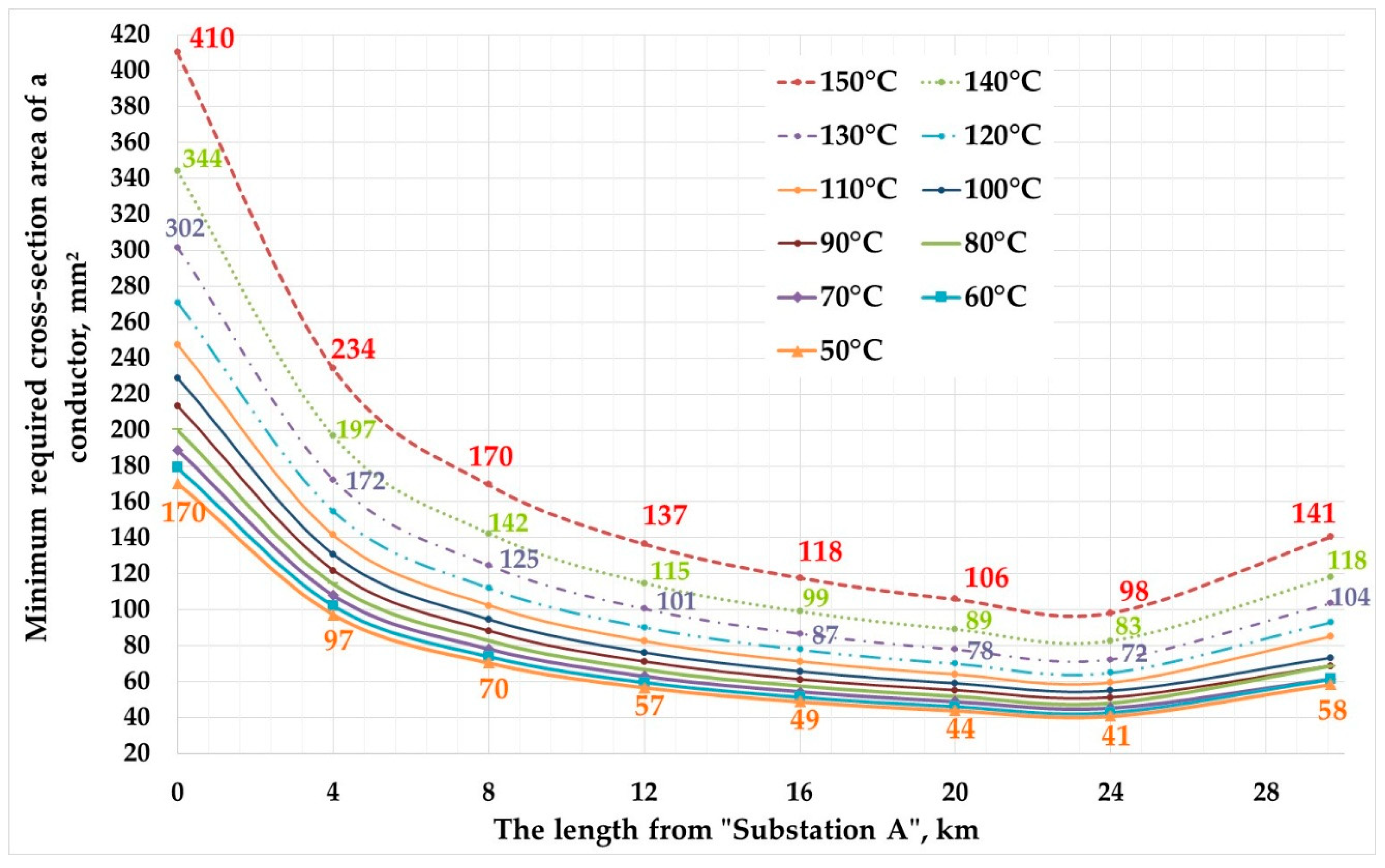
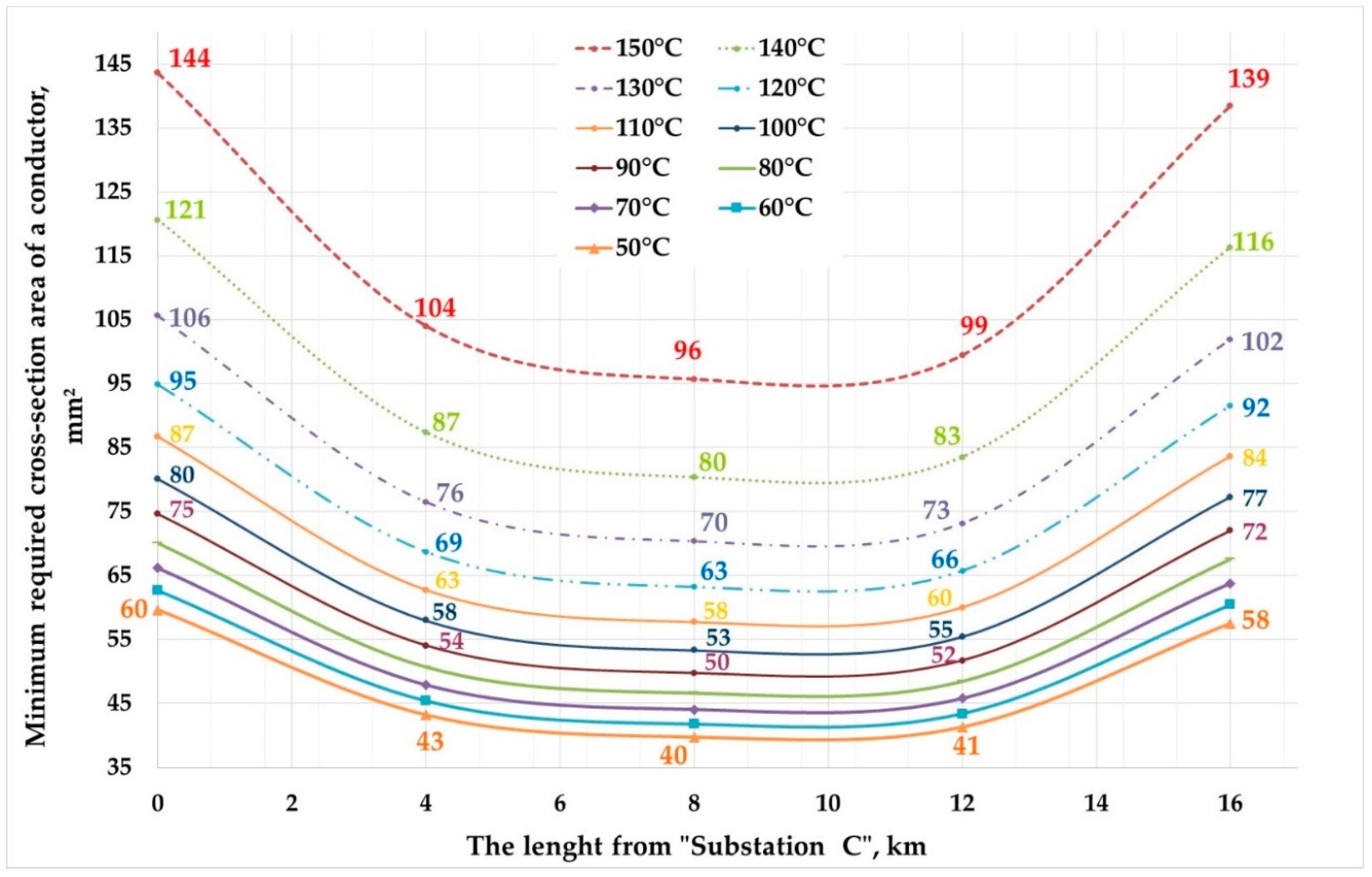
- The comparisons between the cross-sectional areas of the conductor in terms of the OHL length starting from a substation busbar and moving toward the next substation are presented in Table 3 for “OHL No.1” and Table 4 for “OHL No.2”. For instance, when the OHL length was 0–4 km and the phase-to-ground short-circuit (Isc(1)) was considered, the difference between these lengths (0 km and 4 km) in terms of the cross-sectional area of the conductor was 69.1% for “OHL No.1”; however, for “OHL No.2” at the same length range, the value was 30.9%. In another example, when the OHL length was 12–16 km and the three-phase short-circuit (Isc(3)) was considered, the differences between these lengths (12 km and 16 km) in terms of the cross-sectional area of the conductor were 14.8% for “OHL No.1” and 32.8% for “OHL No.2”.
- (b)
- The cross-sectional area analysis of “OHL No.1” shows that, for lengths of 0–8 km, the maximum difference of 84% was observed for 3I0(1,1), with the minimum of 32.1% for Isc(3); for lengths of 8–24 km, the maximum difference of 26% and the minimum difference of 5.3% were found for the same 3I0(1,1), and, for lengths of 24–30 km, the difference was relatively in the same range for all of the examined short-circuit currents (see Table 3).
- (c)
- The total length of “OHL No.2” was less (17 km) than that of “OHL No.1” (30 km). Therefore, the difference did not exceed 32%. For instance, for lengths of 0–4 km, the differences for all of the considered short-circuit currents were almost in the same range. However, for lengths of 4–12 km, the maximum difference of 14.4% was observed for 3I0(1,1), with the minimum of 3.9% for Isc(3); for lengths of 12–16 km, the maximum difference of 32.8% was observed for Isc(3), with the minimum of 26.8% for 3I0(1,1) (see Table 4).
- (d)
- Three times the zero-sequence current and the phase-to-ground short-circuit current had the highest differences in the cross-sectional areas of the conductor in terms of the TL length.
The difference with respect to the initial temperature of a conductor (θi) based on the computed cross-sectional areas of the conductor for all types of the estimated short-circuit currents for both OHLs shows the following results: when the initial temperature of a conductor was taken to be the maximum from 150 °C to 100 °C, the difference between the 10 °C steps decreased; for instance, the difference between 150 °C and 140 °C was 17.4%, and that between 140 °C and 130 °C was 13.2%, followed by differences of 10.7%, 9.1%, and 7.9%. After this temperature range, from 100 °C to 50 °C, the difference continued to decrease and became relatively small: 7.0%, 6.3%, 5.8%, 5.4%, and 5.0%.
4.3. Selection of Required Minimum Cross-Sectional Area of Conductor with Respect to Maximum Short-Circuit Current among the Three Estimated
This part of the paper presents the selection of the cross-sectional area of a conductor with respect to the maximum fault current among the three considered short-circuit currents and according to each initial conductor temperature (11 temperature points). Therefore, along the total length of the OHL, a reasonably appropriate cross-sectional area for the conductor was selected (the biggest cross-sectional area among the three of them).
The obtained results show the following observations (see Figure 6 for “OHL No.1” and Figure 7 for “OHL No.2”, as well as Table 5):
- (a)
- The selection of the cross-sectional area of a conductor was based mainly on the three-phase short-circuit current (Isc(3)) and three times the zero-sequence short-circuit current (3I0(1,1)) by considering the worst-case scenario, i.e., the maximum short-circuit current among the three considered for both OHLs.
- (b)
- The difference with respect to the initial temperature of a conductor (θi) and each length from the initial substation busbar toward another substation had the same range when considering the selected cross-sectional areas of the conductor (worst-case scenario). For instance, when the OHL length was 0–4 km, the difference between these lengths (0 km and 4 km) in terms of the considered cross-sectional area of the conductor was 54.5% for “OHL No.1”; however, for “OHL No.2” at the same length range, it was 32.0%. In another example, when the OHL length was 8–12 km, the differences between these lengths (8 km and 12 km) were 21.5% (“OHL No.1”) and 3.9% (“OHL No.2”).
- (c)
- The maximum difference was observed near the substation busbar, and was quite small—in the middle of the line for both cases. For example, the maximum difference of the cross-sectional area of the conductor was 54.5% for “OHL No.1” (between the zeroth km and fourth km, “Substation A” busbar), whereas, for “OHL No.2”, it was 32.9 % (between the 12th km and 16th km, “Substation B” busbar). The minimum difference was 7.5% for “OHL No.1” (between the 20th km and 24th km, close to the “Substation B” busbar), and the same was observed for “OHL No.2”, with a value of 3.9% (between the 12th km and 16th km, near the “Substation B” busbar).
4.4. Selection of Optimum Cross-Sectional Area of Conductor and Identification of Particular Temperature Regions (TRs) and Length Regions (LRs)
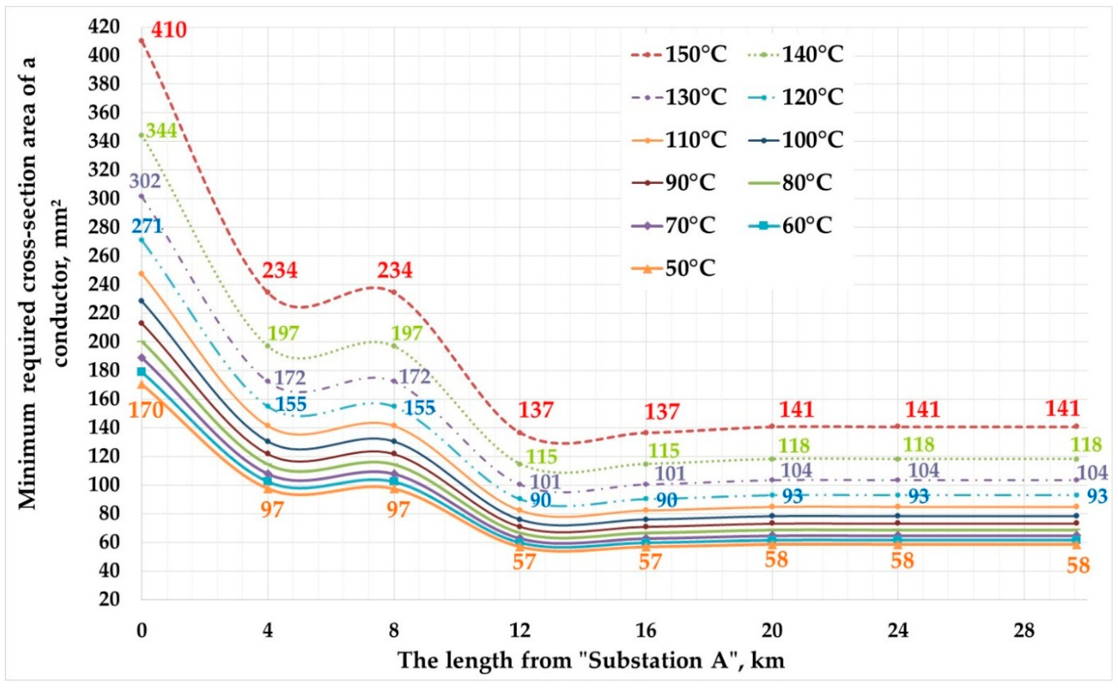
The obtained results related to the selection of the optimum cross-sectional area for the conductor in terms of the initial conductor temperature are presented in Figure 8 for “OHL No.1” and in Figure 9 for “OHL No.2”.
The main concept of this representation was to select the common required minimum conductor cross-sectional area with respect to the maximum short-circuit currents by revealing the overlap regions in terms of the initial conductor temperature, as well as the length of the TL (starting from the substation busbar toward another substation).
- (a)
- The largest cross-sectional areas for a conductor were found for the “OHL No.1” length from the zeroth to fourth km for all the examined initial temperatures of the conductor, where the difference in terms of the cross-sectional area of the conductor was 54.5%. There was no difference between the power line lengths from the fourth to the eighth km. However, a very high difference was observed from the eighth km to the 12th km, which was 52.7%. From the 12th km to the 30th km for the length of “OHL No.1”, there was almost no difference (only 3% from the 16th km to the 20th km).
- (b)
- A similar tendency was observed for “OHL No.2”. For instance, the difference in terms of the cross-sectional area of the conductor had the highest value from the zeroth to the fourth km, which was 32%. There was no difference between the power line lengths from the fourth km to the 12th km. However, from the 12th km to the 17th km for the length of “OHL No.2”, there was a very high difference, which was 28.5%.
Based on the abovementioned results, the following temperature regions (TRs) and length regions (LRs) were identified:
- (1)
- For “OHL No.1”, four TRs and three LRs were applied as follows:
- -
- TR1, with an initial conductor temperature of 150–140 °C;
- -
- TR2: 140–120 °C;
- -
- TR3: 120–80 °C;
- -
- TR4: 80–50 °C;
- -
- LR1, which represents the line from “Substation A” between the zeroth km and fourth km (0–4 km);
- -
- LR2 (4–8 km);
- -
- LR3 (8–30 km), which means that “Substation B” was reached.
- (2)
- For “OHL No.2”, three TRs and three LRs were applied as follows:
- -
- TR1, with an initial conductor temperature of 150–130 °C;
- -
- TR2: 130–80 °C;
- -
- TR3: 80–50 °C;
- -
- LR1, which represents the line from “Substation C” between the zeroth km and fourth km (0–4 km);
- -
- LR2 (4–12 km);
- -
- LR3 (12–16 km), which means that “Substation B” was reached.
The difference between the TRs is especially essential for the high initial temperatures of a conductor. For example, the following factors should be considered:
- (a)
- The minimum required cross-sectional area of a conductor of 240 mm2 should be selected when the initial temperature of the conductor is taken to be at TR1 (150–140 °C) for LR2 (4–8 km). At the same time, when the initial temperature of a conductor decreases, for example to TR3 (120–80 °C), a cross-sectional area of 120 mm2 should be selected for the same LR2 (see Table 6).
- (b)
- The cross-sectional area of a conductor of 150 mm2 should be selected when the initial temperature of the conductor is taken to be at TR1 (150–130 °C) for LR1 (0–4 km). When the initial temperature of the conductor decreases to TR2 (130–80 °C), a cross-sectional area of 120 mm2 should be selected for the same LR1 (see Table 7).
- (c)
- The final choice, which is based on the calculated cross-sectional areas of the conductor, might be not appropriate because of project requirements in terms of the capacity of the OHL. Therefore, it was done by applying larger cross-sections for the conductor compared to the estimated one (see Table 6 and Table 7). Because the comparison was performed for two types of advanced conductors, the closest nominal aluminum cross-sectional area was selected.
Once the cross-sectional areas of the conductor were defined with regard to the fault current limitation, the benefits of the application of the advanced conductors (HTLScs) could be discovered.
5. Results of Application of HTLS Conductors
It was necessary to select the advanced conductor type after the minimum required cross-sectional area of the conductor was identified with respect to the TR and LR. Two types, the aluminum conductor composite reinforced (ACCR) and aluminum conductor composite core (ACCC) [26,37,47,48], were selected by considering the results for the final cross-sectional area of the conductor (see Table 6 and Table 7). These advanced conductors provide cost-effective overhead conductor solutions, in addition to improving the grid efficiency, capacity, reliability, and resilience. The ACCR type relies on a core of aluminum composite wires surrounded by temperature-resistant aluminum–zirconium wires (see Figure 10a) [49]. The ACCC type is based on advanced composite technology and uses a high-strength composite core consisting of carbon and glass fibers embedded in a toughened thermoset resin matrix (see Figure 10b) [50].
The appropriate types of ACCC and ACCR were selected based on the estimated cross-sectional area of the conductor for each TR and LR. The assumptions resulted in almost equal thermal limitation borders and operating conditions for the ACCC and ACCR types.
The data on the selected conductor types can be found in Table 8. The following comments related to these data could be made:
- (a)
- Based on the minimum required cross-sectional area, the ACCC and ACCR types were both selected with larger or almost the same cross-sectional areas for the conductor. There were few cases where the cross-sectional area of the selected conductor was slightly lower than the estimated values. These selections could be justified by a location in the middle of the OHL for these conductors. Moreover, there is a low probability that the estimated short-circuit currents will reach their maximum values.
- (b)
- The ACCC type had a minimum cross-sectional area of 112.8 mm² (ACCC-115), and the ACCR type had an area of 131 mm² (Partridge). Advanced conductors with lower cross-sectional areas than those mentioned above are not manufactured or there was no justification to use them because of several technical restrictions.
- (c)
- All of the cross-sectional areas of the advanced conductor types were selected as close as possible to the estimated values for the minimum required cross-sectional area of a conductor.
- (d)
- For both OHLs, seven types of ACCCs and six types of ACCRs were selected based on the required cross-sectional area of a conductor along the entire power line and according to the estimation conditions.
The OHL project comparison was devoted to the following aspects:
- (1)
- The capacity provided by the selected type of advanced conductor in the considered LR in terms of the initial conductor temperature, i.e., the TR;
- (2)
- The total up-front capital costs for the construction of a new OHL, as well as the reconstruction of the existing one under the assumed computation conditions.
The obtained results for each case study of the OHL project are considered below in a detailed manner.
5.1. Assessment of the Overhead Power Line Project Based on Throughput Capacity
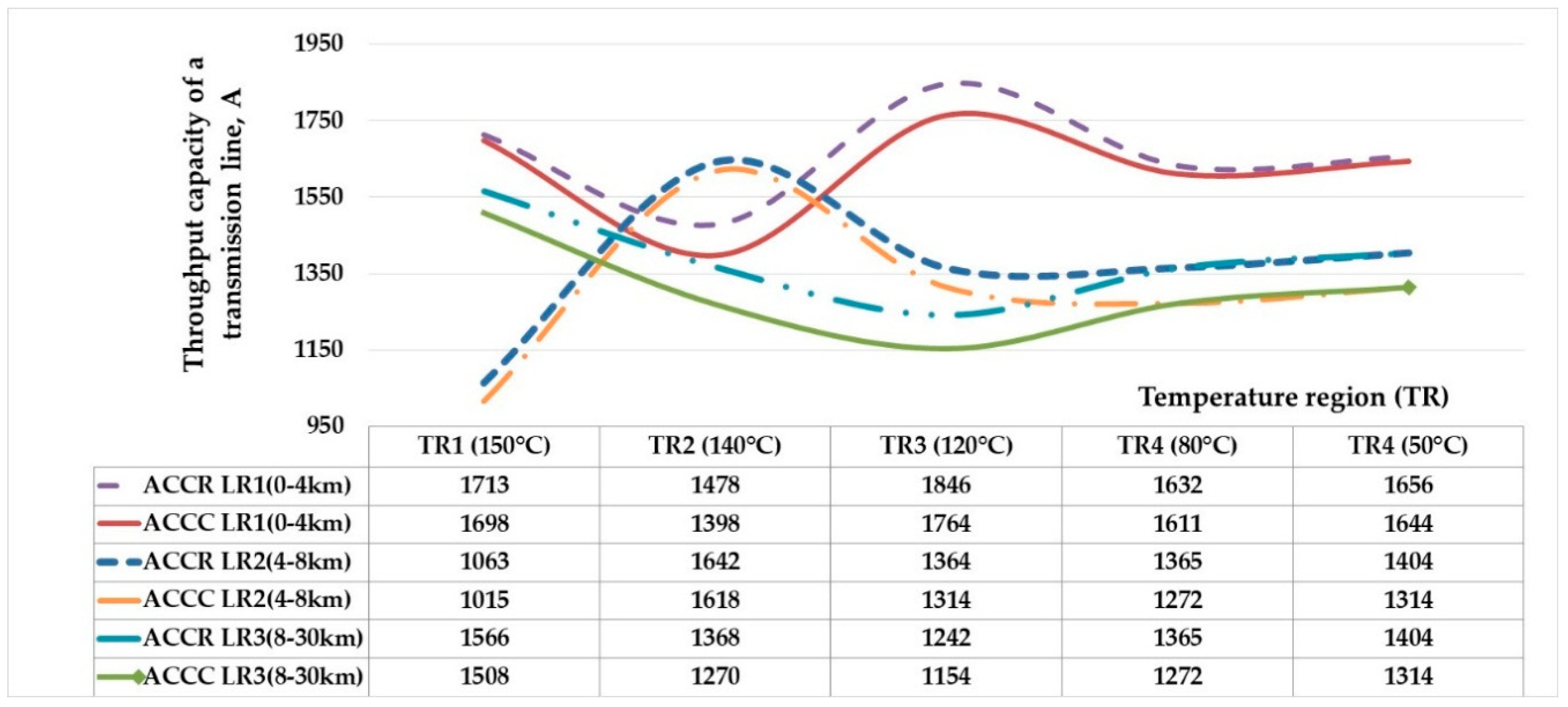
Comparisons of the power line potential capacities of the two types of HTLScs are presented in Figure 11 for “OHL No.1” and Table 9 for “OHL No.2” based on the required throughput current for a 1200 A TL for a single 600 A circuit. The throughput current evaluation considered the previously selected optimum cross-sectional areas for a conductor for the TR and LR in order to ensure the OHL project capacity requirements. Thus, the most economically justified project alternative was selected. For example, when TR2 was examined (the initial conductor temperature was assumed to be a maximum of 140 °C as the worst-case scenario), the throughput current of the TL satisfied the project requirement for both conductor types and all specified LRs. A maximum current of 1642 A was observed for the ACCR type for LR2 (4–8 km), with the minimum current of 1270 A for the ACCC type for LR3 (8–30 km) and “OHL No.1” (see Figure 11). Bundled conductors were used to reach the project requirement, as well as the safe and reliable operation of the OHL.
The same estimation technique was applied for “OHL No.2”. However, the throughput capacity of the examined TL did not vary within one TR, and it remained the same for all LRs. This was due to the relatively short TL length of 17 km. The choice for the cross-sectional area of a conductor should be reasonable for the entire power line length. However, in this case, it remained the same within the same TR, but different for the ACCC and ACCR types. For instance, a maximum current of 1719 A was observed for the ACCR type for TR2 for all the LRs (the same cross-sectional area for the conductor was selected along the whole OHL length), with a minimum current of 1251 A for the ACCC type for TR3 for “OHL No.2” (see Table 9).
It could be concluded that the ACCR type had a better ability to provide higher capacities under specific limitations compared to the ACCC type. However, the following can be observed:
- (a)
- The maximum difference between the throughput capacities was 7.4% when the initial conductor temperature was 140 °C (TR1) for LR3 (8–30 km), and the minimum of 0.7% was found for 50 °C (TR4) and LR1 (0–4 km). This difference had the tendency to decrease for all LRs of the TL when moving closer to the 30th km of “OHL No.1” (toward “Substation B”).
- (b)
- When “OHL No.2” was considered, the maximum difference was 25.1% for TR2 and all the LRs within it. However, the minimum of 0.7% was found TR3 and all the LRs. The cross-sectional area of the conductor was consistent within one TR, as explained above.
5.2. Assessment of Overhead Power Line Project Based on Total Up-Front Capital Costs
The total up-front capital costs of the TL were estimated for two scenarios as follows:
- I.
- Construction of a new OHL;
- II.
- Reconstruction of the existing one, basically by replacing the existing conventional conductor (ACSR) with the HTLSc.
The computation of the up-front capital costs performed as follows:
where
Ccc = ∑Cm + ∑Ci + ∑Coc,
- Ccc is the total up-front capital cost in euros (EUR);
- ∑Cm is the total material cost in EUR;
- ∑Ci is the total installation cost in EUR;
- ∑Coc represents the other costs in EUR.
Total material cost includes the cost of towers and their foundation, conductors and their connections, insulator strings, ground wire, ground cable, and spacers. A major part of the components’ cost was taken from the project specification. For instance, the cost of the towers and their foundation depends basically on the tower type (tension or suspension tower), its height, and its number. The cost of the insulator strings depends on the tower type, as well as OHL voltage. The cost of the ground wire depends on the TL length, purpose (for lightning protection and/or data communication channel), and the tower type and its number, as well as the insulator type and its number. The cost of the ground cable depends on the tower type and its number. The cost of the spacer is included based on a requirement; if the TL has bundled conductors, there are certain instructions to perform calculation of a total number of spacers and, usually, the spacers are used every 50 m along the examined length.
The cost of the conductor depends on the TL length, number of circuits, and number of the conductors in a phase, as well as the particular conductor type. For the connections, the tower type and its number, as well as the insulator type and its number, should considered. In this study, the cost of a conductor was specified by the defined cross-sectional area with respect to the fault current limitation and selected type for the ACCC and ACCR types (see Table 8). Moreover, selection of a type of conductor followed previously defined TRs and LRs (see Table 6 and Table 7).
Installation costs usually vary from 15% to 30% of the total up-front capital costs [53]. These costs depend on the complicity of the TL, which includes consideration of used material for both construction and re-construction scenarios.
Other costs include civil, engineering (approximately 10%), and commission costs (around 1%) [53]. In general, civil costs depend on the tower type, its foundation, and its number, as well as the project requirements (standard) for a width of a right of way.
The material and installation costs of the towers, conductors, ground wire, ground cable, insulator string, and spacer, as well as other costs such as civil engineering and commissioning costs, were fully taken into account for the new OHL construction. However, for the reconstruction of the existing TL, the tower material and installation costs were roughly diminished compared to the new TL—in the case where there was a need for tower reinforcement as a result of the use of a larger cross-sectional area for the conductor.
Detailed cost information was not readily available for the various conductor types, which are listed in Table 8. However, some information provided was based on experts’ opinions, which reflect commonly applied cost differences between the ACCC, ACCR, and ACSR conductors. For instance, an expert opinion explained in Reference [54] stated that the “ACCC that costs two to three times the cost of a conventional ACSR to help reduce a project’s up-front capital cost”. Another example shows a cost comparison of the transmission upgrade for three alternatives: when building a parallel line with ACSR (the conductor cost was 119,000 United States dollars (USD)), when rebuilding a line with twin-bundled ACSR (238,000 USD), and when reconductoring with ACCR (755,000 USD) [55]. Simple calculations show that the cost difference between the examined ACCR and ACSR conductors varied between 6.3 and 3.2. In this way, the price of the ACCC was assumed as two and half times that of the conventional conductor price for the same cross-sectional area of the conductor. The price of the ACCR was taken as five times that of the ACSR cost.
The estimation results of the effect of the advanced conductors (ACCC and ACCR types) and towers on both material cost and total up-front capital costs are summarized in Table 10 (“OHL No.1”) and Table 11 (“OHL No.2”).
- (a)
- If the new “OHL No.1” is constructed, the project with the ACCC type had a maximum effect of 17% and a minimum of 4% of the conductor on the material cost. The project with the ACCR type had a maximum effect of 29% and a minimum of 7%. However, the effect of a tower on the material cost was quite high; for instance, the maximum effect was 89% with a minimum of 78% for the ACCC type, while the maximum was 86% with a minimum of 67% for the ACCR type). Moreover, the effect of the total impact on the total up-front capital costs of the conductor varied from 3.5% to 7.2%, and the effect of the tower varied from 38.4% to 40% for both conductor types. When considering construction of “OHL No.2”, a similar tendency was observed. For instance, the maximum effect of the conductor on the total material cost reached 12.9% with a minimum of 5.7%, while the maximum effect for the weight of the tower was 34.9% with a minimum of 38.2%.
- (b)
- In the case of the reconstruction of the existing power line, the effect of the conductor increased for both material and total up-front capital costs in contrast to the effect of the tower for the examined TLs. For example, the effect of the conductor on the total up-front capital costs varied from 29.4% to 47.1%, and the effect of the tower varied from 16.3% to 22.1% for both conductor types (“OHL No.1”). When “OHL No.2” was considered, the effect of the conductor on the total up-front capital costs varied from 9.0% to 19.4%, and the effect of the tower varied from 6.6% to 7.6%.
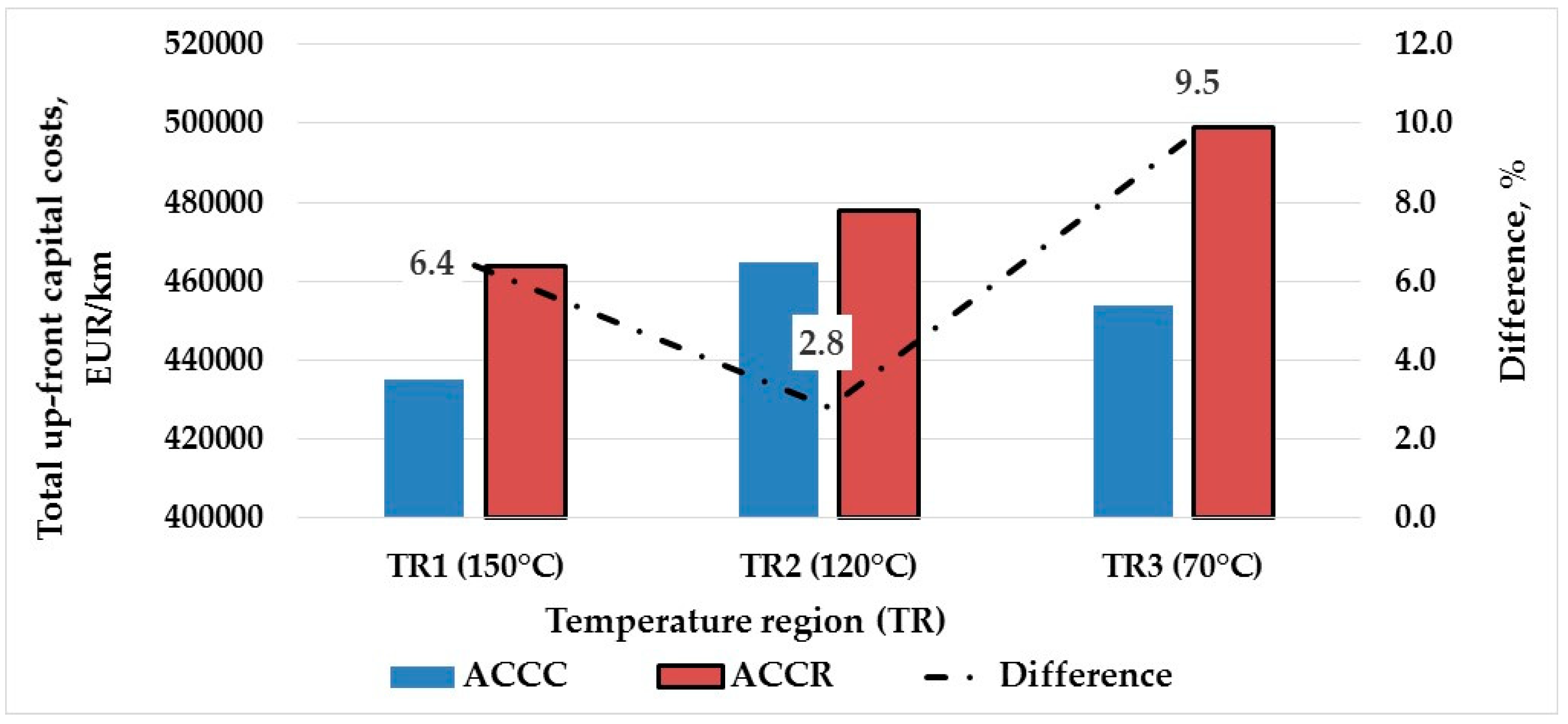
The up-front capital costs were calculated for each power line project, taking into account the final selected cross-sectional area and type for the conductor according to each TR and LR. For instance, the calculation results for “OHL No.1” are presented in Figure 12 for the first scenario (new power line) and in Figure 13 for the second one (reconductoring the existing TL). The up-front capital costs for “OHL No.2” are presented in Figure 14 for the first scenario and in Figure 15 for the second case.
- (1)
- The maximum difference in the OHL project cost reached 4.4% for TR1, where the initial temperature of the conductor was 150 °C (worst-case scenario), and the minimum difference of 1.7% was found for TR4 (50 °C) in the case of the construction of a new OHL.
- (2)
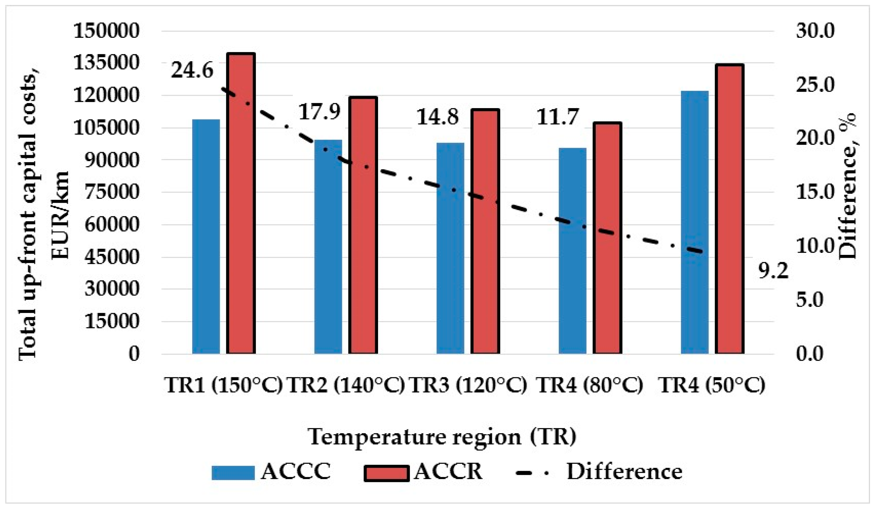
- If the existing power line is reconstructed, the maximum difference will become 24.6% for the same TR1 for the new TL, and the minimum difference will be 9.2% for TR4 due to the higher impact of the conductor cost on the total up-front capital costs of the TL project.
- (3)
- The project with the ACCR type had the maximum up-front capital costs for TR1 (150 °C), but the maximum for the TR4 (50 °C) with the ACCC type. However, the minimums for both the ACCR and ACCC types were for TR4 (80 °C) in both examined scenarios.
- (1)
- If a new OHL is constructed, the maximum difference in the TL cost will reach 6.3% for TR3 (70 °C), and the minimum difference will be 1.8% for TR2 (120 °C).
- (2)
- However, for the second scenario, the maximum difference becomes 9.5% for the same TR1 as in the case of the construction of a new power line, and the minimum difference will be 2.8% for the same TR3.
The project with the ACCR type had the maximum up-front capital costs for TR3 (70 °C); however, with the ACCC type, the maximum was found for TR2 (120 °C) in both considered scenarios. On the other hand, the minimum up-front capital costs were observed for TR1 (150 °C) for both advanced conductor types and examined scenarios.
It can be noted that the first examined scenario—the new OHL construction case—had high up-front capital costs for both advanced conductor types. However, the difference between them was not very large, and the maximum difference was observed for “OHL No.2” and TR3 (70 °C), which was 6.3%. In the second scenario, when the reconductoring of the existing TL was considered, the difference became quite high, with a maximum of 24.6% observed for “OHL No.1” and TR1 (150 °C).
6. Discussion and Conclusions
This evaluation study considered two 110 kV OHL projects with specific requirements: “OHL No.1” (between “Substation A” and “Substation B”, with a total length of 30 km) and “OHL No.2” (between “Substation C” and “Substation B”, with a total length of 17 km).
By adopting the proposed evaluation algorithm, an analysis of the cross-sectional areas selected for the conductor showed that larger cross-sections were calculated for higher short-circuit currents, which were basically observed near the substation busbar, with a smaller one in the middle of the OHL. Secondly, the final selections for the cross-sectional areas for the conductor were mainly based on the three-phase short-circuit currents and three times the zero-sequence currents. Once the optimum cross-sections were found, the TRs and LRs were identified for both OHL projects.
The computed difference with respect to the initial temperature of a conductor (the TRs were considered) between the cross-sectional areas of the conductor for the maximum values (from 150 °C to 100 °C) was higher (minimum is 7.9 %) than that for the later temperature range (from 100 °C to 50 °C), where the difference continued to decrease (maximum of 7%) along the whole length for both OHLs. Four specific temperature regions (TRs) for “OHL No.1” and three TRs for “OHL No.2” were identified with respect to the chosen optimum cross-sectional areas for the conductor under the examined computation conditions.
The calculated difference between the cross-sectional areas of a conductor in terms of the TL length was rather high near a substation busbar and toward the middle of the OHL. However, it was quite low closely to other substation busbar for “OHL No.1”, whereas the results for “OHL No.2” were different. For instance, difference of 54.5% was observed for “OHL No.1” from the zeroth to the fourth km, with a difference of 52.7% from the eighth km to the 12th km. Then, from the 12th km to the 30th km (toward “Substation B”), there was almost no difference (with a difference of only 3% from the 16th km to the 20th km). The highest difference was found from the zeroth to fourth km (32%) for “OHL No.2”, with no difference from the fourth to 12th km; however, a very high difference of 28.5% was observed from the 12th km to 17th km (toward “Substation B”). Three length regions (LRs) were separately identified with respect to the chosen optimum cross-sectional areas of the conductor for each OHL project.
Based on the final selections for the cross-sectional areas of the conductor, as well as the conductor types with respect to the identified TRs and LRs, the up-front capital costs were estimated for each TL project for each scenario. The obtained results showed that the total up-front capital costs were higher when the ACCR types were used, compared to the application of the ACCC types for both considered scenarios (the construction of a new OHL and reconstruction of the existing TL) and for both examined OHL projects. This was because of the relatively high price of the ACCR types compared to the ACCC types (a difference of two times was taken into consideration) and a slight difference in the selected cross-sectional areas, which raised the total costs for the project. For example, when TR1 (150 °C) was considered (worst-case scenario), the up-front capital costs reached the maximum difference of 4.4% between the projects using the ACCC types and ACCR types in the case of the construction of a new TL for “OHL No.1”. For the reconductoring scenario, it was 24.6% for the same TR1, which was caused by the higher impact of the conductor cost on the total costs. The maximum difference of 6.3% for TR3 (70 °C) was found in the case of the new power line construction, and 9.5% was observed for TR1 for the second examined scenario for “OHL No.2”. It is worth noting that the ACCR types had higher throughput capacities than the ACCC types for both OHLs. The difference was rather small (7.4%) for “OHL No.1” (for TR1 and the LR3), but relatively higher for “OHL No.2” (25.1% for TR2 and all the LRs). The presented difference did not greatly impact the decision because both scenarios satisfied the throughput capacity requirements of the TL project. Moreover, the difference curve (between the ACCC and ACCR types) in terms of the total up-front capital costs of 110 kV power line projects had a tendency to decrease with the initial temperature of the conductor. In addition, the effects of the conductor and tower were analyzed on both material cost and total up-front capital costs based on considered scenarios for both OHL projects (ACCC and ACCR types). If a new TL is constructed, the effect of a conductor is quite small compared to the effect of the tower on both total costs. For instance, the effect of the conductor on the total up-front capital costs varied from 3.5% to 7.2% (“OHL No.1”) and from 5.7% to 12.9% (“OHL No.2”) in contrast to the effect of the tower, which varied from 38.4% to 40.0% (“OHL No.1”) and from 34.9% to 38.2% (“OHL No.2”). However, for the case of the reconstruction of the existing OHL, the situation changed in the opposite way, whereby the effect of the conductor largely increased compared to the effect of the tower for both power lines. For example, the effect of the conductor on the total up-front capital costs varied from 29.4% to 47.1%, and the effect of the tower varied from 16.3% to 22.1% (“OHL No.1”), a similar tendency to that observed for “OHL No.2”. In spite of a small effect of the conductor on the total up-front capital costs in the case of a new TL construction (commonly, it reached up to 30%), the proposed concept shows an economically justified solution with respect to the selection of an optimum cross-sectional area and type of conductor (LRs and DRs consideration), unlike traditional selection of a conductor, typically done once and commonly for a whole length of the transmission line (oversize).
Selecting the cross-sectional area of the conductor with respect to the fault current limitation in advance provides the potential opportunity to increase the protection level, as well as the effective operation of a power line. This idea has possible practical application because of the physical ability of an HTLSc to be able to withstand high conductor temperatures. In this way, a preliminary consideration of the fault current limitation benefits the operation of the OHL under abnormal conditions such as overloading and overheating.
The proposed evaluation algorithm for the power line project extends the hidden operational limits for a transmission network and provides an additional technical prospective for the integration of new technologies into a smart grid. Likewise, this study could profitably be considered in relation to transmission network planning issues on the short-, medium-, and long-term horizons.
Future work will include a consideration of different OHL projects under various technical requirements to reveal the strong relationship of the main impacts (random parameters, parameter uncertainty, etc.), nature of any change, and identification of the common factors and criteria with respect to decision-making in terms of transmission network planning optimization tasks. The proposed method will be improved based on the discovered considerations and assumptions.
Funding
This research received no external funding.
Conflicts of Interest
The author declares no conflicts of interest.
References
- Verseille, J.; Staschus, K. ENTSO-E and European TSO cooperation in operations, planning, and R&D. IEEE Power Energy Mag. 2015, 13, 21–29. [Google Scholar]
- Hinkel, P.; Ostermann, M.; Pluntke, H.; Raoofsheibani, D.; Wellssow, W.; Gies, A. Development of a 2025 operational Central European transmission system model to investigate grid restoration strategies. In Proceedings of the International ETG Congress, Bonn, Germany, 28–29 November 2017; pp. 1–6. [Google Scholar]
- Kariniotakis, G.; Martini, L.; Caerts, C.; Brunner, H.; Retiere, N. Challenges, innovative architectures and control strategies for future networks: The web-of-cells, fractal grids and other concepts. CIRED Open Access Proc. J. 2017, 2017, 2149–2152. [Google Scholar] [CrossRef]
- European Commission. Energy roadmap 2050. In Luxembourg: Publications Office of the European Union; European Commission: Brussels, Belgium, 2012; p. 20. ISBN 978-9-27921798-2. [Google Scholar] [CrossRef]
- Western Area Power Administration (WAPA). Transmission Enhancement Technology Report. In Upper Great Plains Region, Transmission System Planning; WAPA: Lakewood, CO, USA, 2002; p. 17. [Google Scholar]
- Buijs, P.; Bekaert, D.; Cole, S.; Hertem, D.V.; Belmans, R. Transmission investment problems in Europe: Going beyond standard solutions. Energy Policy 2011, 39, 1794–1801. [Google Scholar] [CrossRef]
- Public Service Commission of Wisconsin. Environmental Impacts on Transmission lines. 31p. Available online: https://psc.wi.gov/Documents/Brochures/Enviromental%20Impacts%20TL.pdf (accessed on 12 January 2019).
- Rosellón, J. Different approaches towards electricity transmission expansion. Rev. Netw. Econ. 2003, 2, 238–269. [Google Scholar] [CrossRef]
- Krishnan, V.K.; Ho, J.; Hobbs, B.; Liu, A.L.; Mccalley, J.; Shahidehpour, M.; Zheng, Q.P. Co-optimization of electricity transmission and generation resources for planning and policy analysis: Review of concepts and modeling approaches. Energy Syst. 2016, 7, 297–332. [Google Scholar] [CrossRef]
- Munoz, F.D.; Watson, J.P.; Hobbs, F. Optimizing your options: Extracting the full economic value of transmission when planning under uncertainty. Electr. J. 2015, 28, 26–38. [Google Scholar] [CrossRef]
- Dong, X.; Kang, C.; Zhang, N.; Yan, H.; Meng, J.; Niu, X.; Tian, X. Estimating life-cycle energy payback ratio of overhead transmission line toward low carbon development. J. Mod. Power Syst. Clean Energy 2015, 3, 123–130. [Google Scholar] [CrossRef]
- Tokombayev, A.; Heydt, G.T. HTLS Upgrades and payback for the economic operation improvement of power transmission systems. Electr. Power Compon. Syst. 2015, 43, 345–355. [Google Scholar] [CrossRef]
- Patel, H.B. Re-conductoring scenario & payback calculations of acsr moose and its equivalents conductors for 400 kV transmission line [thermal uprating]. Int. J. Adv. Eng. Res. Dev. 2015, 2, 1283–1290. [Google Scholar]
- Teegala, S.K.; Singal, S.K. Economic analysis of power transmission lines using interval mathematics. J. Electr. Eng. Technol. 2015, 10, 1471–1479. [Google Scholar] [CrossRef]
- Kiessling, F.; Nefzger, P.; Nolasco, J.F.; Kaintzyk, U. Overhead Power Lines: Planning, Design, Construction, 1st ed.; Springer: Berlin/Heidelberg, Germany; New York, NY, USA, 2003; pp. 195–228. ISBN 978-36-4205556-0. [Google Scholar]
- Varygina, A.O.; Savina, N.V. The influence of new functional properties of active-adaptive electrical networks on the correctness of selection and verification of conductor cross-sections by existing methods. In Proceedings of the IEEE International Multi-Conference on Industrial Engineering and Modern Technologies (FarEastCon), Vladivostok, Russia, 3–4 October 2018; pp. 1–5. [Google Scholar] [CrossRef]
- Beryozkina, S.; Petrichenko, L.; Sauhats, A.; Guseva, S.; Neimane, V. The stochastic approach for conductor selection in transmission line development projects. In Proceedings of the IEEE International Energy Conference (ENERGYCON), Cavtat, Croatia, 13–16 May 2014; pp. 557–564. [Google Scholar] [CrossRef]
- Beryozkina, S.; Petrichenko, L.; Sauhats, A.; Jankovskis, N. Overhead power line design in market conditions. In Proceedings of the IEEE 5th International Conference on Power Engineering, Energy and Electrical Drives (POWERENG), Riga, Latvia, 11–13 May 2015; pp. 278–282. [Google Scholar] [CrossRef]
- Sauhats, A.; Beryozkina, S.; Petrichenko, L.; Neimane, V. Stochastic optimization of power line design. In Proceedings of the IEEE PowerTech Conference, Eindhoven, The Netherlands, 29 June–2 July 2015; pp. 1–6. [Google Scholar] [CrossRef]
- Dama, D.; Muftic, D.; Vajeth, R. Conductor optimisation for overhead transmission lines. In Proceedings of the IEEE Power Engineering Society Inaugural Conference and Exposition, Durban, South Africa, 11–15 July 2005; pp. 410–416. [Google Scholar] [CrossRef]
- Vasconcelos, J.A.D.; Teixeira, D.A.; Ribeiro, M.F.D.O. Optimal selection and arrangement of cables for compact overhead transmission lines of 138/230 kV. IEEE Latin Am. Trans. 2017, 15, 1460–1466. [Google Scholar] [CrossRef]
- CENELEC. Conductors for overhead lines. Round wire concentric lay stranded conductors; EN 50182: 2001/AC:2013; European Committee for Electrotechnical Standardization (CENELEC): Brussels, Belgium, August 2013; p. 78. [Google Scholar]
- Avdaković, S. Advanced Technologies, Systems, and Applications III, Proceedings of the International Symposium on Innovative and Interdisciplinary Applications of Advanced Technologies (IAT), Volume 1; Springer: Basel, Switzerland, 2019; pp. 187–197. ISBN 978-3-03-002573-1. [Google Scholar] [CrossRef]
- Kühnel, C.; Bardl, R.; Stengel, D.; Kiewitt, W.; Grossmann, S. Investigations on the mechanical and electrical behaviour of HTLS conductors by accelerated ageing tests. CIRED Open Access Proc. J. 2017, 2017, 273–277. [Google Scholar] [CrossRef]
- De Paulis, F.; Olivieri, C.; Orlandi, A.; Giannuzzi, G.; Bassi, F.; Morandini, C.; Fiorucci, E.; Bucci, G. Exploring remote monitoring of degraded compression and bolted joints in HV power transmission lines. IEEE Trans. Power Deliv. 2016, 31, 2179–2187. [Google Scholar] [CrossRef]
- CTC Global Corporation. Engineering Transmission Lines with High Capacity Low Sag ACCC Conductors, 1st ed.; CTC Global: Irvine, CA, USA, 2011; pp. 17–18, 97–106. ISBN 978-0-61-557959-7. [Google Scholar]
- CTC Global Corporation. ACCC Conductor Installation Guidelines; WI-750-070; CTC Global: Irvine, CA, USA, 2017; 8p. [Google Scholar]
- Kwon, J.; Hedman, K.W. Transmission expansion planning model considering conductor thermal dynamics and high temperature low sag conductors. IET Gener. Transm. Distrib. 2015, 9, 2311–2318. [Google Scholar] [CrossRef]
- Da Silva, A.A.P.; Bezerra, J.M.B. A model for uprating transmission lines by using HTLS conductors. IEEE Trans. Power Deliv. 2011, 26, 2180–2188. [Google Scholar] [CrossRef]
- Beryozkina, S.; Sauhats, A. Research and simulation of overhead power line uprating using advanced conductors. In Proceedings of the 56th International Scientific Conference on Power and Electrical Engineering of Riga Technical University (RTUCON), Riga, Latvia, 14 October 2015; pp. 1–4. [Google Scholar] [CrossRef]
- Silva, A.A.P.; Bezerra, J.M.B. Applicability and limitations of ampacity models for HTLS conductors. Electr. Power Syst. Res. 2012, 93, 61–66. [Google Scholar] [CrossRef]
- Exposito, A.G.; Santos, J.R.; Romero, P.C. Planning and operational issues arising from the widespread use of HTLS conductors. IEEE Trans. Power Syst. 2007, 22, 1446–1455. [Google Scholar] [CrossRef]
- Albizu, I.; Mazon, A.J.; Valverde, V.; Buigues, G. Aspects to take into account in the application of mechanical calculation to high-temperature low-sag conductors. IET Gener. Transm. Distrib. 2010, 4, 631–640. [Google Scholar] [CrossRef]
- Agrawal, S.; Nigam, M.K. Lightning phenomena and its effect on transmission line. Recent Res. Sci. Technol. 2014, 6, 183–187. [Google Scholar]
- Panth, D. Reasons for failure of transmission lines and their prevention strategies. Int. J. Electr. Electron. Data Commun. 2014, 2, 1–4. [Google Scholar]
- Ratnamahilan, P.; Hoole, P.R.P. Modeling the lightning earth flash return stroke for studying its effects on engineering systems. IEEE Trans. Mag. 1993, 29, 1839–1844. [Google Scholar] [CrossRef]
- Electric Power Research Institute (EPRI). Demonstration of Advanced Conductors for Overhead Transmission Lines; EPRI: Palo Alto, CA, USA, 2008; p. 1017448. [Google Scholar]
- AST, The Kurzeme Ring. Available online: http://www.ast.lv/en/transmission-network-projects/kurzeme-ring (accessed on 12 January 2019).
- Baltic Energy Market Interconnection Plan (BEMIP), 6th Progress Report, July 2013–August 2014. p. 54. Available online: https://ec.europa.eu/energy/sites/ener/files/documents/20142711_6th_bemip_progress_report.pdf (accessed on 12 January 2019).
- Ma, G.; Li, C.; Quan, J.; Jiang, J.; Cheng, Y. A fiber Bragg grating tension and tilt sensor applied to icing monitoring on overhead transmission lines. IEEE Trans. Power Deliv. 2011, 26, 2163–2170. [Google Scholar] [CrossRef]
- Savadjiev, K.; Farzaneh, M. Modeling of icing and ice shedding on overhead power lines based on statistical analysis of meteorological data. IEEE Trans. Power Deliv. 2004, 19, 715–721. [Google Scholar] [CrossRef]
- Ma, G.-M.; Li, Y.-B.; Mao, N.-Q.; Shi, C.; Zhang, B.; Li, C.-R. A fiber Bragg grating based dynamic tension detection system for overhead transmission line galloping. Sensors 2018, 18, 365. [Google Scholar] [CrossRef] [PubMed]
- Power Line Systems. PLS-CADD—Version 13.2, User’s Manual. 2014, p. 540. Available online: http://www.powline.com/products/pls_cadd.html (accessed on 12 January 2019).
- CENELEC. Overhead Electrical Lines Exceeding AC 45 kV. Part 1: General Requirements—Common Specifications; EN 50341-1/A1; European Committee for Electrotechnical Standardization (CENELEC): Brussels, Belgium, July 2009; pp. 106–112. [Google Scholar]
- Lomane, T.; Rubcovs, S.; Kovalenko, S.; Berzina, K. The effectiveness increasing of earth fault distance protection operation in high-voltage cable line. In Proceedings of the 9th International Scientific Symposium on Electrical Power Engineering (ELEKTROENERGETIKA), Stara Lesna, Slovakia, 12–14 September 2017; pp. 378–383. [Google Scholar]
- Blackburn, J.L.; Domin, T.J. Protective Relaying: Principles and Applications, 4th ed.; Taylor & Francis Inc.: Boca Raton, FL, USA, 2014; 324p, ISBN 9781439888117. [Google Scholar]
- Gorur, R.; Mobasher, B.; Olsen, R. Characterization of Composite Cores for High Temperature-Low Sag (HTLS) Conductors (Final project report); Power Systems Engineering Research Center (PSERC): Tempe, AZ, USA, July 2009. [Google Scholar]
- Banerjee, K. Making the Case for High Temperature Low Sag (HTLS) Overhead Transmission Line Conductors. Master’s Thesis, Arizona State University, Tempe, AZ, USA, 2014. [Google Scholar]
- 3M Aluminum Conductor Composite Reinforced (ACCR). Available online: https://www.ieee.hr/_download/repository/Allan_Russell_3M_ACCR_%28Aluminum_Conductor_Composite_Reinforced%29_-_Proven_Solutions_to_Increase_Capacity.pdf (accessed on 12 January 2019).
- CTC Global’s High Performance Conductors for a Low Carbon World™. Available online: https://www.ctcglobal.com/?_vsrefdom=adwords&gclid=EAIaIQobChMIqvH_0Ifp3wIVxjLTCh3muA9XEAAYASAAEgK-0_D_BwE (accessed on 12 January 2019).
- ACCR Conductor. Available online: https://www.3m.com/3M/en_US/power-transmission-us/resources/accr-technical/ (accessed on 15 January 2019).
- ACCC Conductor. Available online: https://www.ctcglobal.com/accc-conductor/ (accessed on 9 January 2019).
- Yli-Hannuksela, J. The Transmission Line Cost Calculation. Ph.D. Thesis, Vaasan Ammattikorkeakoulu, University of Applied Sciences, Vaasan, Finland, 2011; pp. 36–41. [Google Scholar]
- Bryant, D. High cost vs. high performance. How a pricier product can save you money. Utility Prod. Mag. 2014, 11, 4. [Google Scholar]
- Glenmar, E. Cambri, 3M ACCR. More Amps—More Confidence, 2012, 9p. Available online: https://d2oc0ihd6a5bt.cloudfront.net/wp-content/uploads/sites/837/2015/06/HTLS-DDW-ADB-3M-ACCR-PreR11.pdf (accessed on 28 February 2019).
Figure 1.
Kurzeme Ring project location.

Figure 2.
Estimated short-circuit currents along 110 kV “overhead power line (OHL) No.1” from “Substation A” (zeroth km) toward “Substation B” (30th km).
Figure 2.
Estimated short-circuit currents along 110 kV “overhead power line (OHL) No.1” from “Substation A” (zeroth km) toward “Substation B” (30th km).

Figure 3.
Estimated short-circuit currents along 110 kV “OHL No.1” from “Substation B” (30th km) toward “Substation A” (zeroth km).
Figure 3.
Estimated short-circuit currents along 110 kV “OHL No.1” from “Substation B” (30th km) toward “Substation A” (zeroth km).
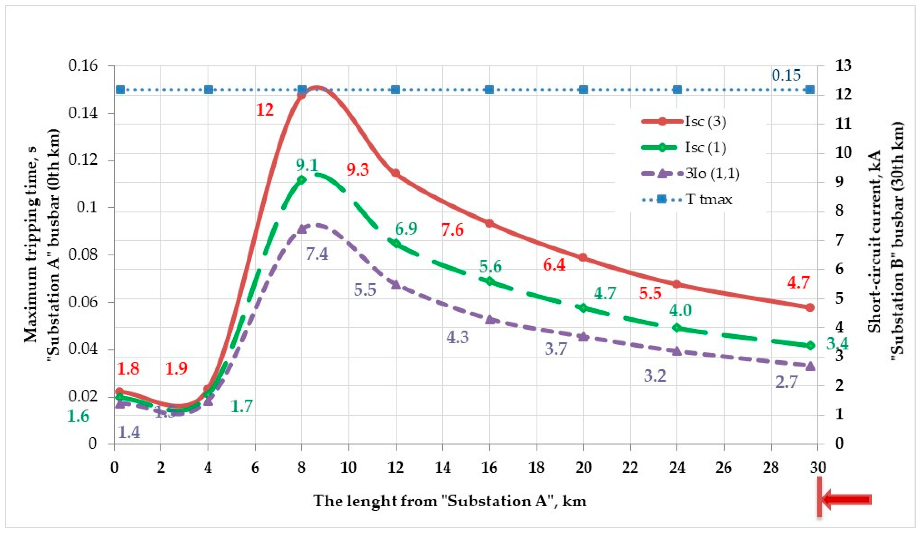
Figure 4.
Estimated short-circuit currents along 110 kV “OHL No.2” from “Substation C” (zeroth km) toward “Substation B” (17th km).
Figure 4.
Estimated short-circuit currents along 110 kV “OHL No.2” from “Substation C” (zeroth km) toward “Substation B” (17th km).
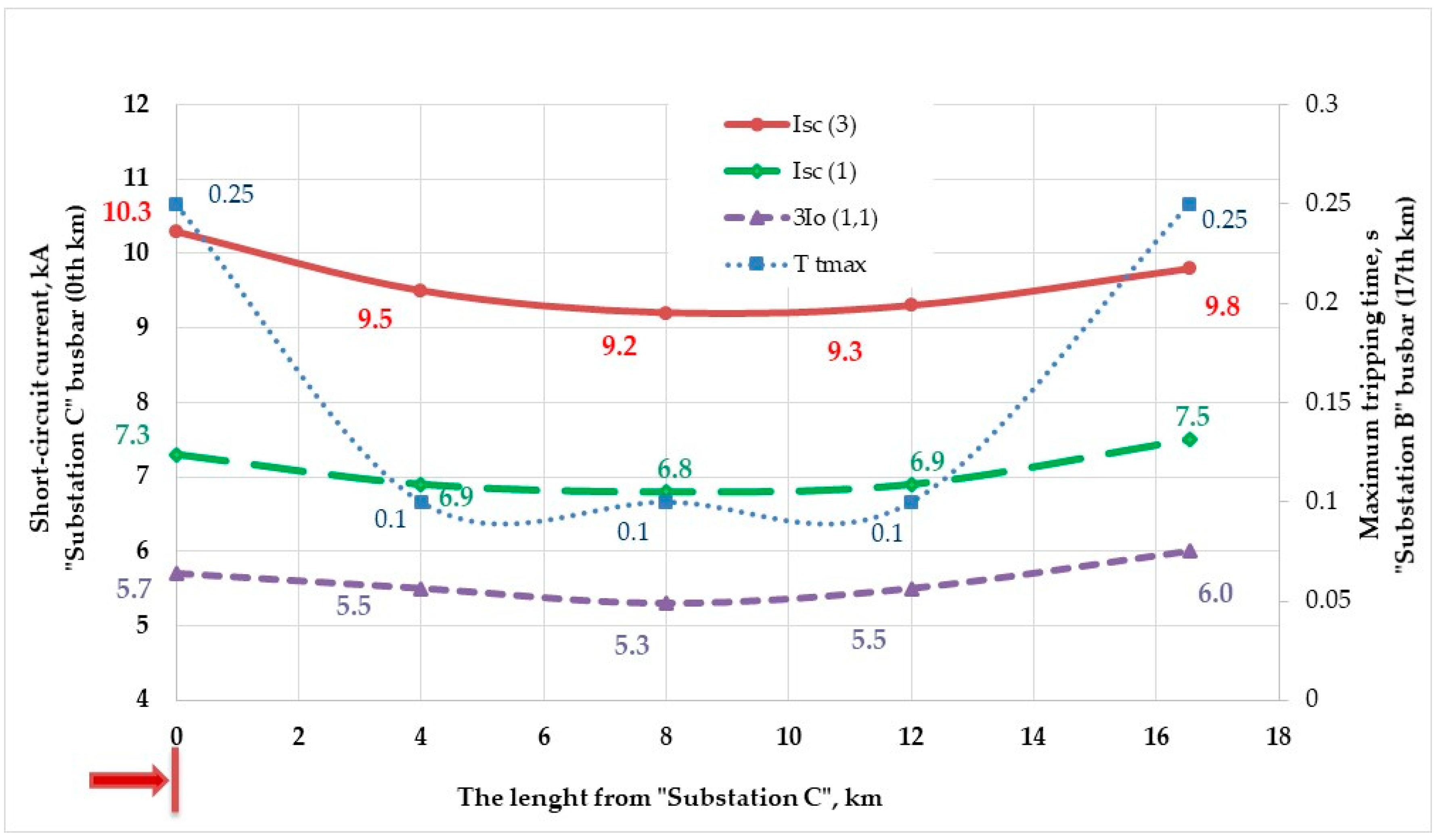
Figure 5.
Estimated short-circuit currents along 110 kV “OHL No.2” from “Substation B” (17th km) toward “Substation C” (zeroth km).
Figure 5.
Estimated short-circuit currents along 110 kV “OHL No.2” from “Substation B” (17th km) toward “Substation C” (zeroth km).

Figure 6.
Selected cross-sectional areas of conductor along “OHL No.1” from “Substation A” (zeroth km) toward “Substation B” (30th km).
Figure 6.
Selected cross-sectional areas of conductor along “OHL No.1” from “Substation A” (zeroth km) toward “Substation B” (30th km).

Figure 7.
Selected cross-sectional areas of conductor along “OHL No.2” from “Substation C” (zeroth km) toward “Substation B” (17th km).
Figure 7.
Selected cross-sectional areas of conductor along “OHL No.2” from “Substation C” (zeroth km) toward “Substation B” (17th km).

Figure 8.
Identification of overlaps of cross-sectional areas of conductor for “OHL No.1”.

Figure 9.
Identification of overlaps of cross-sectional areas of conductor for “OHL No.2”.
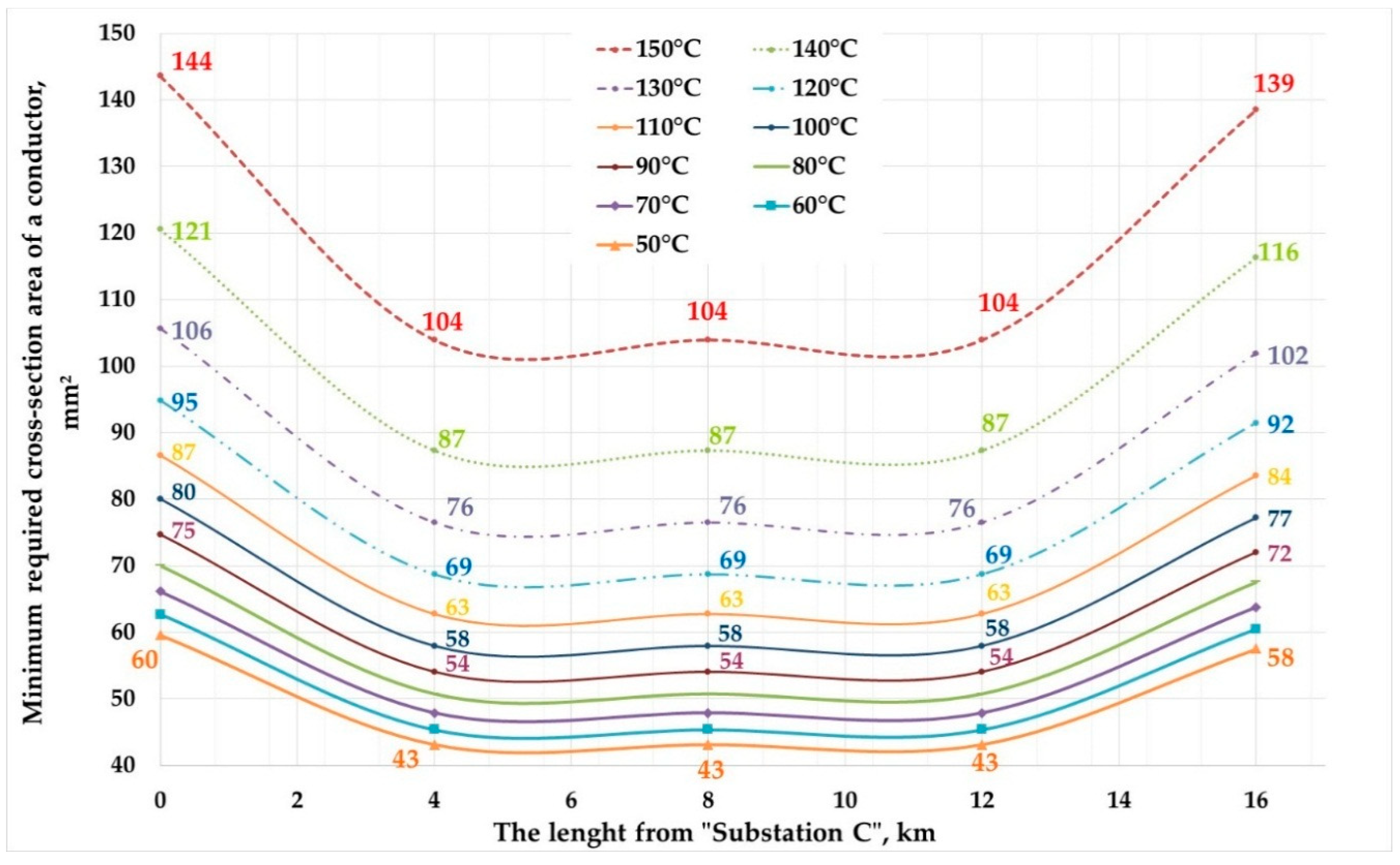
Figure 10.
Conductor configurations of (a) aluminum conductor composite reinforced (ACCR) type [51] and (b) aluminum conductor composite core (ACCC) type [52].
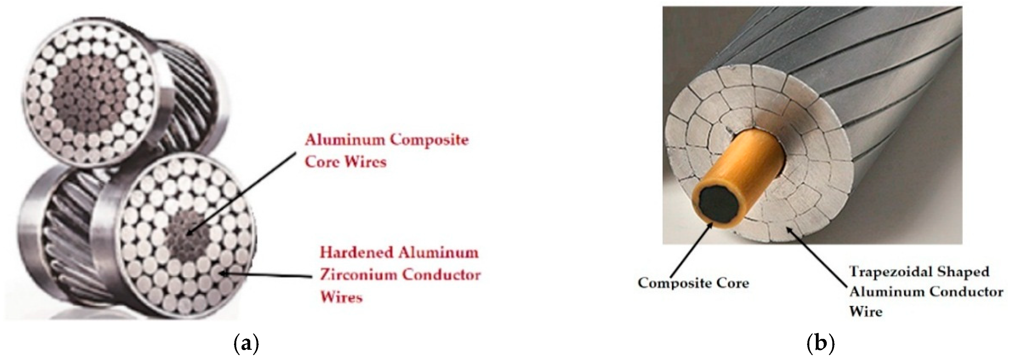
Figure 11.
Capacity comparison of ACCC and ACCR types based on selected final cross-sectional areas of conductor for “OHL No.1”.
Figure 11.
Capacity comparison of ACCC and ACCR types based on selected final cross-sectional areas of conductor for “OHL No.1”.

Figure 12.
Total up-front capital costs for construction of a new transmission line (TL) for “OHL No.1” case.
Figure 12.
Total up-front capital costs for construction of a new transmission line (TL) for “OHL No.1” case.
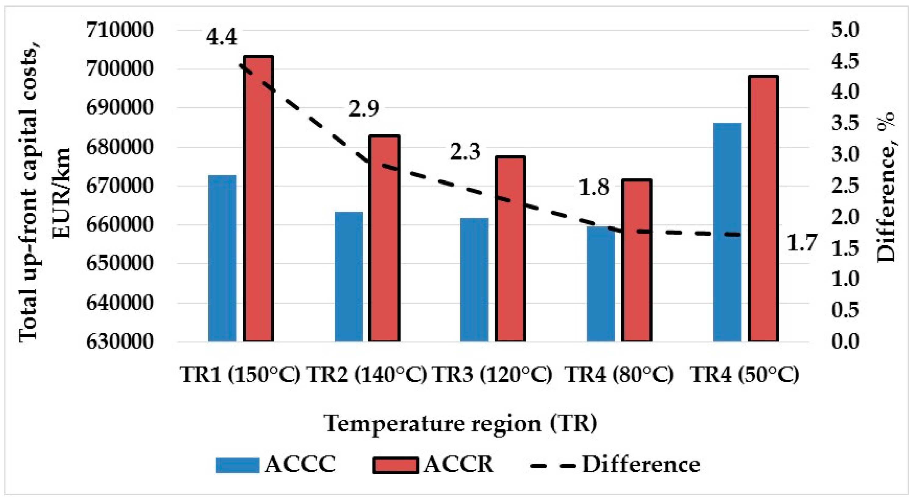
Figure 13.
Total up-front capital costs for reconstruction of existing power line for “OHL No.1” case.
Figure 13.
Total up-front capital costs for reconstruction of existing power line for “OHL No.1” case.

Figure 14.
Total up-front capital costs for construction of a new TL for “OHL No.2” case.
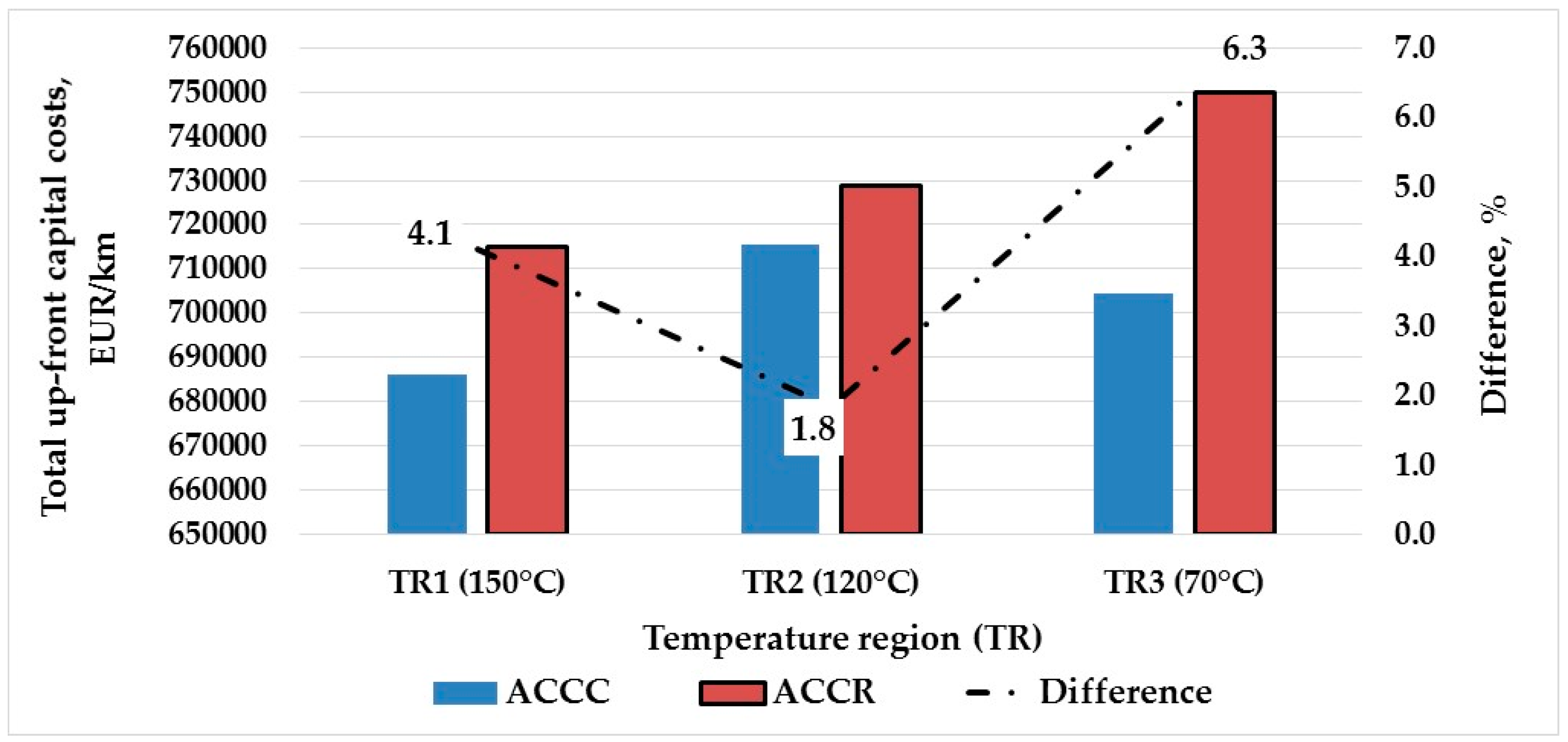
Figure 15.
Total up-front capital costs for reconstruction of existing power line for “OHL No.2” case.
Figure 15.
Total up-front capital costs for reconstruction of existing power line for “OHL No.2” case.

Table 1.
Calculated minimum required cross-sectional area of conductor for “overhead power line (OHL) No.1” based on three estimated short-circuit currents.
Table 1.
Calculated minimum required cross-sectional area of conductor for “overhead power line (OHL) No.1” based on three estimated short-circuit currents.
| θi, °C | Length from “Substation A”, km 1 | S for Isc(1), mm 2 | S for Isc(3), mm 2 | S for 3I0(1,1), mm 2 | θi, °C | Length from “Substation A”, km 2 | S for Isc(1), mm 2 | S for Isc(3), mm 2 | S for 3I0(1,1), mm 2 |
|---|---|---|---|---|---|---|---|---|---|
| 150 | 0 | 400 | 384 | 410 | 100 | 0 | 223 | 214 | 229 |
| 4 | 194 | 234 | 168 | 4 | 108 | 131 | 93 | ||
| 8 | 129 | 170 | 105 | 8 | 72 | 95 | 59 | ||
| 12 | 101 | 137 | 81 | 12 | 56 | 76 | 45 | ||
| 16 | 86 | 118 | 67 | 16 | 48 | 66 | 38 | ||
| 20 | 77 | 106 | 61 | 20 | 43 | 59 | 34 | ||
| 24 | 72 | 98 | 58 | 24 | 40 | 55 | 32 | ||
| 30 | 106 | 141 | 85 | 30 | 59 | 79 | 47 | ||
| 140 | 0 | 335 | 322 | 344 | 90 | 0 | 208 | 199 | 213 |
| 4 | 163 | 197 | 141 | 4 | 101 | 122 | 87 | ||
| 8 | 108 | 142 | 88 | 8 | 67 | 88 | 55 | ||
| 12 | 85 | 115 | 68 | 12 | 53 | 71 | 42 | ||
| 16 | 73 | 99 | 57 | 16 | 45 | 61 | 35 | ||
| 20 | 65 | 89 | 51 | 20 | 38 | 55 | 30 | ||
| 24 | 61 | 83 | 48 | 24 | 38 | 51 | 30 | ||
| 30 | 89 | 118 | 71 | 30 | 55 | 73 | 44 | ||
| 130 | 0 | 294 | 282 | 302 | 80 | 0 | 195 | 187 | 200 |
| 4 | 143 | 172 | 123 | 4 | 95 | 114 | 82 | ||
| 8 | 95 | 125 | 77 | 8 | 63 | 83 | 51 | ||
| 12 | 74 | 101 | 59 | 12 | 49 | 67 | 39 | ||
| 16 | 64 | 87 | 50 | 16 | 42 | 58 | 33 | ||
| 20 | 57 | 78 | 45 | 20 | 36 | 52 | 28 | ||
| 24 | 53 | 72 | 42 | 24 | 35 | 48 | 28 | ||
| 30 | 78 | 141 | 62 | 30 | 52 | 69 | 41 | ||
| 120 | 0 | 264 | 253 | 271 | 70 | 0 | 184 | 177 | 189 |
| 4 | 128 | 155 | 111 | 4 | 90 | 108 | 77 | ||
| 8 | 85 | 112 | 69 | 8 | 59 | 78 | 48 | ||
| 12 | 67 | 90 | 53 | 12 | 47 | 63 | 37 | ||
| 16 | 57 | 78 | 45 | 16 | 40 | 54 | 37 | ||
| 20 | 51 | 70 | 40 | 20 | 36 | 49 | 28 | ||
| 24 | 48 | 65 | 38 | 24 | 33 | 45 | 27 | ||
| 30 | 70 | 93 | 56 | 30 | 49 | 65 | 39 | ||
| 110 | 0 | 241 | 231 | 247 | 60 | 0 | 174 | 167 | 179 |
| 4 | 117 | 141 | 101 | 4 | 85 | 102 | 73 | ||
| 8 | 78 | 102 | 63 | 8 | 56 | 74 | 46 | ||
| 12 | 61 | 82 | 49 | 12 | 44 | 60 | 35 | ||
| 16 | 52 | 71 | 41 | 16 | 38 | 51 | 29 | ||
| 20 | 47 | 64 | 37 | 20 | 34 | 46 | 27 | ||
| 24 | 44 | 59 | 35 | 24 | 31 | 43 | 25 | ||
| 30 | 64 | 85 | 51 | 30 | 46 | 61 | 37 | ||
| 50 | 0 | 166 | 159 | 170 | 50 | 16 | 36 | 49 | 28 |
| 4 | 81 | 97 | 70 | 20 | 32 | 44 | 25 | ||
| 8 | 53 | 70 | 44 | 24 | 30 | 41 | 24 | ||
| 12 | 42 | 57 | 34 | 30 | 44 | 58 | 35 |
1 Column No.2 reflects the length from “Substation A” for the initial temperature of a conductor of 150 °C, 140 °C, 130 °C, 120 °C, 110 °C, or 50 °C (partially). 2 Column No.7 reflects that for temperatures of 100 °C, 90 °C, 80 °C, 70 °C, 60 °C, or 50 °C (continuous).
Table 2.
Calculated minimum required cross-sectional area of conductor for “OHL No.2” based on three estimated short-circuit currents.
Table 2.
Calculated minimum required cross-sectional area of conductor for “OHL No.2” based on three estimated short-circuit currents.
| θi, °C | Length from “Substation C”, km 1 | S for Isc(1), mm 2 | S for Isc(3), mm 2 | S for 3I0(1,1), mm 2 | θi, °C | Length from “Substation C”, km 2 | S for Isc(1), mm 2 | S for Isc(3), mm 2 | S for 3I0(1,1), mm 2 |
|---|---|---|---|---|---|---|---|---|---|
| 150 | 0 | 104 | 144 | 82 | 90 | 0 | 54 | 75 | 43 |
| 4 | 76 | 104 | 60 | 4 | 39 | 54 | 31 | ||
| 8 | 71 | 96 | 56 | 8 | 37 | 50 | 29 | ||
| 12 | 78 | 99 | 64 | 12 | 41 | 52 | 33 | ||
| 16 | 105 | 139 | 84 | 16 | 55 | 72 | 44 | ||
| 140 | 0 | 87 | 121 | 69 | 80 | 0 | 51 | 70 | 40 |
| 4 | 64 | 87 | 51 | 4 | 37 | 51 | 29 | ||
| 8 | 59 | 80 | 47 | 8 | 35 | 47 | 27 | ||
| 12 | 69 | 83 | 54 | 12 | 38 | 49 | 31 | ||
| 16 | 89 | 116 | 71 | 16 | 51 | 68 | 41 | ||
| 130 | 0 | 76 | 106 | 60 | 70 | 0 | 45 | 66 | 38 |
| 4 | 56 | 76 | 44 | 4 | 33 | 48 | 28 | ||
| 8 | 52 | 70 | 41 | 8 | 31 | 44 | 26 | ||
| 12 | 57 | 73 | 47 | 12 | 34 | 46 | 30 | ||
| 16 | 78 | 102 | 62 | 16 | 46 | 64 | 30 | ||
| 120 | 0 | 68 | 95 | 54 | 60 | 0 | 43 | 63 | 36 |
| 4 | 50 | 69 | 40 | 4 | 32 | 45 | 26 | ||
| 8 | 47 | 63 | 37 | 8 | 29 | 42 | 24 | ||
| 12 | 51 | 66 | 42 | 12 | 32 | 43 | 28 | ||
| 16 | 70 | 92 | 56 | 16 | 44 | 60 | 37 | ||
| 110 | 0 | 63 | 87 | 50 | 50 | 0 | 43 | 60 | 34 |
| 4 | 46 | 63 | 36 | 4 | 32 | 43 | 25 | ||
| 8 | 43 | 58 | 34 | 8 | 29 | 40 | 23 | ||
| 12 | 47 | 60 | 39 | 12 | 32 | 41 | 27 | ||
| 16 | 64 | 84 | 51 | 16 | 44 | 58 | 35 | ||
| 100 | 0 | 58 | 80 | 46 | |||||
| 4 | 42 | 58 | 34 | ||||||
| 8 | 39 | 53 | 31 | ||||||
| 12 | 43 | 55 | 36 | ||||||
| 16 | 59 | 77 | 47 |
1 Column No.2 reflects the length from “Substation C” for the initial temperature of a conductor of 150 °C, 140 °C, 130 °C, 120 °C, 110 °C, or 100 °C. 2 Column No.7 reflects that for temperatures of 90 °C, 80 °C, 70 °C, 60 °C, or 50 °C.
Table 3.
Comparison between cross-sectional areas of conductor for “OHL No.1”.
| Length from “Substation A”, km | Difference in Cross-Sectional Areas of a Conductor in Terms of Examined Short-Circuit Current, % | ||
|---|---|---|---|
| Isc(1) | Isc(3) | 3I0(1,1) | |
| 0–4 | 69.1 | 48.3 | 84.0 |
| 4–8 | 40.7 | 32.1 | 46.0 |
| 8–12 | 23.9 | 21.5 | 26.0 |
| 12–16 | 15.7 | 14.8 | 18.1 |
| 16–20 | 11.3 | 10.6 | 10.3 |
| 20–24 | 6.7 | 7.5 | 5.3 |
| 24–30 | 38.1 | 35.5 | 38.1 |
Table 4.
Comparison between cross-sectional areas of conductor for “OHL No.2”.
| Length from “Substation C”, km | Difference in Cross-Sectional Areas of a Conductor in Terms of Examined Short-Circuit Current, % | ||
|---|---|---|---|
| Isc(1) | Isc(3) | 3I0(1,1) | |
| 0–4 | 30.9 | 32.0 | 30.9 |
| 4–8 | 7.0 | 8.3 | 7.8 |
| 8–12 | 9.6 | 3.9 | 14.4 |
| 12–16 | 30.1 | 32.8 | 26.8 |
Table 5.
Comparison between selected cross-sectional areas of conductor for both OHLs.
| Length from the Initially Considered Substation Busbar toward Another Substation, km | Difference in the Cross-Sectional Areas of a Conductor for Both OHLs, % | |
|---|---|---|
| “OHL No.1” (30 km) | “OHL No.2” (17 km) | |
| 0–4 | 54.5 | 32.0 |
| 4–8 | 32.1 | 8.3 |
| 8–12 | 21.5 | 3.9 |
| 12–16 | 14.8 | 32.9 |
| 16–20 | 10.6 | - |
| 20–24 | 7.5 | - |
| 24–30 | 35.5 | - |
Table 6.
Final selection of cross-sectional area of conductor for “OHL No.1”. TR—temperature region; LR—length region.
Table 6.
Final selection of cross-sectional area of conductor for “OHL No.1”. TR—temperature region; LR—length region.
| Length from “Substation A”, km | Cross-Sectional Area of Conductor, mm2 | |||
|---|---|---|---|---|
| TR1 (150–140 °C) | TR2 (140–120 °C) | TR3 (120–80 °C) | TR4 (80–50 °C) | |
| LR 1 (0–4) | 410 | 302 | 247 | 189 |
| LR 2 (4–8) | 234 | 172 | 141 | 108 |
| LR 3 (8–30) | 137 | 101 | 93 (122.7 1) | 65 (122.7 1) |
1 The larger nominal aluminum cross-sectional area was adopted (as an example).
Table 7.
Final selection of cross-sectional area of conductor for “OHL No.2”.
| Length from “Substation C”, km | Cross-Sectional Area of Conductor, mm2 | ||
|---|---|---|---|
| TR1 (150–130 °C) | TR2 (130–80 °C) | TR3 (80–50 °C) | |
| LR 1 (0–4) | 144 (150.5 1) | 95 (112.8 1) | 66 (172.3 1) |
| LR 2 (4–12) | 104 (150.5 1) | 69 (112.8 1) | 48 (172.3 1) |
| LR 3 (12–16) | 139 (150.5 1) | 92 (112.8 1) | 64 (172.3 1) |
1 The larger nominal aluminum cross-sectional area was adopted (as an example).
Table 8.
Cross-sectional areas of examined aluminum conductor composite core (ACCC) types and aluminum conductor composite reinforced (ACCR) types for both OHLs.
Table 8.
Cross-sectional areas of examined aluminum conductor composite core (ACCC) types and aluminum conductor composite reinforced (ACCR) types for both OHLs.
| ACCC 1 | ACCR 1 | ||
|---|---|---|---|
| Name | Conductor Cross-Sectional Area, mm² | Name | Conductor Cross-Sectional Area, mm² |
| Curlew | 523.4 | 1033-T13 | 523.4 |
| Grosbeak | 416.2 | Drake | 417.5 |
| Glasgow | 236.7 | Hawk | 238.2 |
| Zadar | 177.4 | Linnet | 172.3 |
| Helsinki | 150.6 | Ostrich | 150.5 |
| Silvassa | 122.7 | Partridge | 131.0 |
| ACCC-115 | 112.8 | ||
1 The actual configuration of a given size of the chosen ACCC types and ACCR types may vary depending on the conductor manufacturer, which may result in slight variations in some of the indicated values.
Table 9.
Capacity comparison of ACCC and ACCR types based on selected final cross-sectional areas of conductor for “OHL No.2”.
Table 9.
Capacity comparison of ACCC and ACCR types based on selected final cross-sectional areas of conductor for “OHL No.2”.
| Length from “Substation C”, km | Throughput Capacity of “OHL No.2”, A | |||||
|---|---|---|---|---|---|---|
| TR1 (150–130 °C) | TR2 (130–80 °C) | TR3 (80–50 °C) | ||||
| ACCC | ACCR | ACCC | ACCR | ACCC | ACCR | |
| LR 1 (0–4) | 1394 | 1444 | 1335 | 1719 | 1251 | 1260 |
| LR 2 (4–12) | 1394 | 1444 | 1335 | 1719 | 1251 | 1260 |
| LR 3 (12–16) | 1394 | 1444 | 1335 | 1719 | 1251 | 1260 |
Table 10.
Comparison of the effects of two main components on the total material cost and up-front capital costs for “OHL No.1”, which connects “Substation A” and “Substation B”.
Table 10.
Comparison of the effects of two main components on the total material cost and up-front capital costs for “OHL No.1”, which connects “Substation A” and “Substation B”.
| Length from “Substation A”, km | Temperature Region, °C | Construction of a New Power Line | Reconstruction of the Existing Power Line | ||||||
|---|---|---|---|---|---|---|---|---|---|
| ACCC | ACCR | ACCC | ACCR | ||||||
| C 1, % | T 2, % | C, % | T, % | C, % | T, % | C, % | T, % | ||
| LR 1 (0–4) | TR1 (150–140) | 17 | 78 | 29 | 67 | 49 | 36 | 66 | 25 |
| LR 2 (4–8) | 9 | 84 | 16 | 78 | 28 | 49 | 43 | 39 | |
| LR 3 (8–30) | 5 | 88 | 10 | 84 | 37 | 18 | 53 | 13 | |
| Total impact 3 | 4.6 | 39.6 | 7.2 | 38.4 | 36.3 | 20.3 | 47.1 | 16.3 | |
| LR 1 (0–4) | TR2 (140–120) | 11 | 83 | 20 | 75 | 37 | 45 | 54 | 33 |
| LR 2 (4–8) | 6 | 86 | 11 | 81 | 20 | 52 | 33 | 44 | |
| LR 3 (8–30) | 4 | 89 | 7 | 86 | 30 | 20 | 45 | 16 | |
| Total impact | 3.7 | 39.9 | 5.5 | 39.1 | 31.3 | 22.0 | 40.4 | 18.6 | |
| LR 1 (0–4) | TR3 (120–80) | 8 | 85 | 15 | 79 | 29 | 48 | 43 | 38 |
| LR 2 (4–8) | 6 | 86 | 11 | 82 | 20 | 52 | 32 | 44 | |
| LR 3 (8–30) | 4 | 89 | 7 | 86 | 30 | 20 | 45 | 16 | |
| Total impact | 3.5 | 40.0 | 5.2 | 39.2 | 30.1 | 22.1 | 38.5 | 19.1 | |
| LR 1 (0–4) | TR4 (80–50) | 6 | 87 | 10 | 83 | 22 | 53 | 34 | 44 |
| LR 2 (4–8) | 4 | 87 | 8 | 84 | 15 | 55 | 26 | 48 | |
| LR 3 (8–30) | 4 | 89 | 7 | 86 | 30 | 19 | 45 | 16 | |
| Total impact | 3.5 | 39.9 | 4.9 | 39.3 | 29.4 | 21.9 | 36.58 | 19.2 | |
1 The effect of a conductor (C, %) on the total material cost in %. 2 The effect of a tower and its foundation (T, %) on the total material cost. 3 Total impact represents effect (sum of the material cost and installation cost for conductor and tower accordantly) on the total up-front capital costs of the examined power line project.
Table 11.
Comparison of the effects of two main components on the total material cost and up-front capital costs for “OHL No.2”, which connects “Substation C” and “Substation B”.
Table 11.
Comparison of the effects of two main components on the total material cost and up-front capital costs for “OHL No.2”, which connects “Substation C” and “Substation B”.
| Length from “Substation C”, km | Temperature Region, °C | Construction of a New Power Line | Reconstruction of the Existing Power Line | ||||||
|---|---|---|---|---|---|---|---|---|---|
| ACCC | ACCR | ACCC | ACCR | ||||||
| C 1, % | T 2, % | C, % | T, % | C, % | T, % | C, % | T, % | ||
| LR 1 (0–4) | TR1 (150–130) | 10 | 84 | 18 | 77 | 34 | 46 | 50 | 35 |
| LR 2 (4–12) | 11 | 83 | 19 | 75 | 44 | 30 | 60 | 21 | |
| LR 3 (12–16) | 9 | 84 | 17 | 77 | 32 | 44 | 48 | 34 | |
| Total impact 3 | 5.7 | 38.2 | 9.2 | 36.7 | 9.0 | 7.6 | 14.2 | 7.1 | |
| LR 1 (0–4) | TR2 (130–80) | 15 | 79 | 19 | 76 | 45 | 37 | 51 | 33 |
| LR 2 (4–12) | 16 | 77 | 20 | 74 | 55 | 23 | 60 | 20 | |
| LR 3 (12–16) | 14 | 79 | 17 | 76 | 43 | 36 | 49 | 33 | |
| Total impact | 9.0 | 36.6 | 10.5 | 35.9 | 14.0 | 7.1 | 16.1 | 6.9 | |
| LR 1 (0–4) | TR3 (80–50) | 15 | 79 | 25 | 69 | 44 | 38 | 60 | 27 |
| LR 2 (4–12) | 16 | 78 | 27 | 67 | 53 | 24 | 69 | 16 | |
| LR 3 (12–16) | 14 | 80 | 24 | 71 | 42 | 37 | 59 | 26 | |
| Total impact | 7.7 | 37.2 | 12.9 | 34.9 | 12.0 | 7.2 | 19.4 | 6.6 | |
1, 2, 3 See the explanation given in the caption of Table 10.
© 2019 by the author. Licensee MDPI, Basel, Switzerland. This article is an open access article distributed under the terms and conditions of the Creative Commons Attribution (CC BY) license (http://creativecommons.org/licenses/by/4.0/).
Share and Cite
MDPI and ACS Style
Beryozkina, S. Evaluation Study of Potential Use of Advanced Conductors in Transmission Line Projects. Energies 2019, 12, 822. https://doi.org/10.3390/en12050822
AMA Style
Beryozkina S. Evaluation Study of Potential Use of Advanced Conductors in Transmission Line Projects. Energies. 2019; 12(5):822. https://doi.org/10.3390/en12050822
Chicago/Turabian StyleBeryozkina, Svetlana. 2019. "Evaluation Study of Potential Use of Advanced Conductors in Transmission Line Projects" Energies 12, no. 5: 822. https://doi.org/10.3390/en12050822
Note that from the first issue of 2016, this journal uses article numbers instead of page numbers. See further details here.