Prediction Modeling and Analysis of Knocking Combustion using an Improved 0D RGF Model and Supervised Deep Learning

Abstract

The knock phenomenon is one of the major hindrances for enhancing the thermal efficiency in spark-ignited engines. Due to the stochastic behavior of knocking combustion, analytical cycle studies are required. However, there are many problems to be addressed with regard to the individual cycle analysis of in-cylinder pressure data. This study thus proposes novel, comprehensive and efficient methodologies for evaluating the knocking combustion in the internal combustion engine. The proposed methodologies include a filtering method for the in-cylinder pressure, the determination of the knock onset, and the calculation of the residual gas fraction. Consequently, a smart knock onset model with high accuracy could be developed using a supervised deep learning that was not available in the past. Moreover, an improved zero-dimensional (0D) estimation model for the residual gas fraction was developed to obtain better accuracy for closed system analysis. Finally, based on a cyclic analysis, a knock prediction model is suggested; the model uses 0D ignition delay correlation under various experimental conditions including aggressive cam phase shifting by a dual variable valve timing (VVT) system. Using the proposed analysis method, insight into stochastic knocking combustion can be obtained, and a faster combustion speed can lead to a higher knock intensity in a steady-state operation.

1. Introduction

In a spark-ignited (SI) engine, increasing the compression ratio is one of the most promising methods to enhance the indicated thermal efficiency (ITE) [1]. To cope with strict global emission standards, the target compression ratio has been increased in recent production engines along with the aggressive utilization of harsh-conditioned operations. However, the engine operation in such conditions is accompanied by increases in the pressure and temperature of the unburned gas region, which results in autoignition or knock phenomena [2].

Knock is a type of spontaneous ignition that occurs in the unburned end-gas region in the cylinder [2]. In the SI engine, as the in-cylinder pressure increases due to the combustion, the temperature of the unburned end-gas ahead of the flame is increased. Hot spots in the end-gas located in front of the flame are autoignited before the flame arrives and cause a spontaneous heat release of the end-gas. The pressure wave generated by the hot spot hits the inside wall of the cylinder and causes a pinging sound. If the heat release is rapid and large enough, it can cause erosion and damage such as piston crown melting, ring cranking, head gasket leakage and bore scuffing [3,4,5].

Knock has to be suppressed, as it provokes engine failure problems and can make the driver uncomfortable when it is strong [3]. Knock avoidance is generally achieved by utilizing a retarded ignition timing. However, this normally deteriorates the work extraction and increases the exhaust loss. Therefore, an enhancement in the ITE can be achieved if the knock can be efficiently suppressed. As the mitigation of the knock is directly related to an increase in the ITE, there have been countless studies on knock suppression.

For a deeper understanding of the knock phenomenon, an analysis based on the in-cylinder pressure is essential. However, the engine knock has a stochastic behavior [6,7]. For instance, the knock occurrence and timing persistently vary even under steady-state operation, when maintaining all of the operating parameters. Therefore, a cyclic approach is required to achieve data from the knocking condition.

First, to precisely designate the in-cylinder pressure value when knock occurs, a method for knock onset (KO) determination is necessary. The definition of the KO is the timing of the knock occurrence, and previous research on it is presented in Section 1.1. However, a description of the detailed logic was excluded to minimize the complexity of the paper, as it is adequately presented in the cited references. With several attempts, conventional methods could provide reasonable KO values from combustion data. However, as they were validated in particular operating conditions (mainly heavy knock conditions), the proper extraction of the KO was not possible in relatively weak knock conditions. Therefore, to increase the preciseness of the KO determination and simultaneously secure the universality, a smart KO model using supervised deep learning is presented in this study.

Along with the mitigation of the knock, its control is also an important factor for achieving a higher ITE in SI engines. Proper control has a great potential for appropriate knock avoidance with a smaller deterioration of the efficiency, and it may allow the utilization of deflagration to enhance the ITE thanks to the instantaneous consumption of the unburned air-fuel mixture. In real driving, because the engine runs in transient conditions, the operating parameters such as the fuel input mass and intake pressure vary rapidly. Therefore, the control has to rely on the instantaneous data, which has to be based on an individual cycle analysis with a proper estimation of the in-cylinder pressure. The residual gas fraction (RGF) has a great influence on the cyclic analysis as it changes not only the in-cylinder gas properties but also the total trapped mass. Because the RGF value has a great impact on the whole processes of the closed system such as compression and combustion, it is significantly necessary to develop a reliable zero-simensional (0D) RGF model for a high-fidelity analysis. Section 1.2 provides a brief review of previous research on 0D RGF modeling, and an improved modeling of the RGF is provided in this study. In addition, this paper focuses on technical proposals to analyze the individual cycle data including a filtering method for in-cylinder pressure profile.

Empirical models for knock prediction have been improved by many researchers to correctly predict the timing of the knock occurrence. The developed models are described in Section 1.3. However, due to the uncertainty of the in-cylinder conditions of the closed system, they applied an average in-cylinder temperature and pressure that were generally obtained by simulation methods. Although the established models show high accuracy, instantaneously obtained conditions have to be used to utilize the models for knock control in actual transient operating conditions, as previously described. Therefore, in this study, the applicability of prediction modeling is also examined based on an individual cycle analysis. In addition, for universality, it will be verified in a wide range of experimental conditions including aggressive valve timing changes using a dual variable valve timing (VVT) system.

This study consists of five sections, including this introduction. Next, literature reviews on KO models, RGF models and knock prediction models are presented. In the next section, the configurations for the engine experiment are described. The detailed engine specifications and operating conditions are listed, and an explanation of the test facility is provided. A discussion of the knock propensity and KO follows in Section 3 that shows how the knock occurrence is determined in this study, and a smart knock onset model with high accuracy is given. In Section 4, detailed methodologies and techniques for the analysis of the knocking combustion are shown, including an improvement of the 0D RGF model. After that, a knock prediction modeling based on previous methodologies is described. Finally, insight into knocking combustion will be presented, based on an established cyclic analysis and knock prediction model.

1.1. Determination of Knock Onset

The threshold value exceeded (TVE) method is used to determine the KO as the timing at which a filtered pressure signal value initially exceeds a certain threshold. Worret et al. [8] showed that the TVE method does not necessarily provide a correct KO. Lee [9] judged the KO as the position where the constant value (3 CA) was biased from the TVE KO. Shahlari and Ghandhi [10] presented a signal energy ratio (SER) method that uses integral of squared pressure oscillation (ISPO) values to compensate for the limitations of the TVE method. In their research, the KO was defined as the timing at which the SER has the highest value (reached a plateau), a proper window size of 5 CA was suggested, and various filters were tested for the high fidelity.

Kim [11] discovered that the SER method can possibly determine a KO earlier than the actual value, so an attempt at modifying the TVE method was made to increase the accuracy. To avoid bias by the Butterworth high-pass filter, a median and a smoothing filter were sequentially applied for 10 data points corresponding to 1 CA in 0.1 CA resolution data. A new threshold (μ+5σ) was set as five times the standard deviation (σ) added to the mean value (μ) from 5 CA before the initially guessed point of the KO. It was concluded that the KO was reached if the value of the data point exceeds the threshold.

Shahlari et al. [10] developed a new algorithm for determining the KO with very high accuracy using an iteration method. A linear fitting method was introduced to capture a separation point in the in-cylinder pressure curve that can be regarded as a sudden increase due to autoignition.

1.2. Zero-Dimensional Residual Gas Fraction Models

Numerous modeling approaches have also been developed to estimate the residual gas fraction [12,13,14]. However, the first research on the valve overlap was attempted by Fox et al. [15]. In this study, an assumption was made that the residual gas was trapped by burned gas in the clearance volume and back flow of the exhaust gas. A new parameter named the valve overlap factor (OF) was proposed, and its impact on the RGF value was considered. The OF is expressed in Equation (1), where $D$ is the valve diameter and $L$ is the valve lift. It denotes the average valve curtain area during valve overlap. Based on an ideal Otto cycle, the model also considers the manifold pressure, compression ratio and engine speed:

$$OF=\frac{D_{IN}{{\displaystyle \int }}_{{\theta }_{IVO}}^{L_{IN}=L_{EX}}{L}_{IN}d\theta +D_{EX}{{\displaystyle \int }}_{L_{IN}=L_{EX}}^{{\theta }_{EVC}}{L}_{EX}d\theta }{V_d}$$

(1)

In a recent study, Kale et al. [16] developed an RGF model in the dual cam phasing condition that distinguishes the valve overlap duration considering the location of the TDC (Top dead center) and timing with the same intake/exhaust valve curtain area. Although this model has many coefficients (13) that must be adjusted, it provided relatively accurate results.

1.3. Knock Prediction Models

To predict the timing at which the knock occurs, autoignition prediction models are being used in many studies. There are mainly three types of prediction model [17]: models using a detailed chemical kinetic mechanism [18], models using simplified mechanisms such as the shell knock model [19,20], and phenomenological models based on the Arrhenius equation. Among the various models, phenomenological models are widely used due to convenience and a fast calculation speed. Assuming a one-step reaction mechanism, the autoignition delay time can be described using the Arrhenius equation. The first attempt at using this method was conducted by Livengood and Wu [21]. Assuming that the reaction is zero-order and the reaction rate does not change, the relationship between the concentration and autoignition delay can be expressed as Equation (2), where $\tau$ is the ignition delay and $\left(x\right)/\left(x_c\right)$ is the concentration ratio. In their studies, it was found that autoignition occurs when the RHS of the equation reaches unity:

$$\frac{\left(x\right)}{(x_c)} ={{\displaystyle \int }}_{t=0}^{t=t_e}\frac{1}{\tau }dt$$

(2)

Zero-dimensional ignition delay correlations are widely used in engine operating conditions due to their great advantage of fast calculation and applicability for the utilization of the Livengood-Wu integral method in actual engine conditions. The first and the most recent correlations are listed in

Table 1. Zero-dimensional ignition delay correlations.

Reference	Formulation	Considerations
Douaud and Eyzat [22]	$\tau =18.69{\left(\frac{ON}{100}\right)}^{3.4017}{p}^{-1.7}exp\left(\frac{3800}{T}\right)$	Octane number
Hoepke et al. [29]	$\tau =8.449\times {10}^{-5}{\left(\frac{P}{T}\right)}^{-1.343}{\left(1-x_{egr}\right)}^{-0.8881}exp\left(\frac{5266}{T}\right)$	Cooled exhaust gas recirculation (EGR)
Chen et al. [17]	$\tau =5.35\times {10}^{-5}{\left(\frac{P}{T}\right)}^{-2.374}{\left(1-x_{egr}\right)}^{-3.013}{\lambda }^{-1.927}exp\left(\frac{3167}{T}\right)$	Cooled EGR Air-fuel ratio
McKenzie et al. [30]	$\tau =2.71\times {10}^{-5}{\left(\frac{P}{T}\right)}^{-1.73}exp\left(\frac{5190}{T}\right){\left(1-w_d\right)}^{-0.618},$ where $wd=x_{egr}+x_{residual}+0.95\left|\frac{\lambda -1}{\lambda +{\left(A/F\right)}_{stoi}}\right|$	Cooled EGR Residual gas Air-fuel ratio

. Douaud and Eyzat [22] proposed a chemical reaction-based ignition delay time calculation and calculated the coefficients by experimental studies using primary reference fuels (iso-octane and n-heptane mixtures). Since the first attempt by Douaud and Eyzat, many studies have used these correlations [8,11,23,24,25,26]. Wayne et al. [27] recalibrated the coefficients, and Pipitone et al. [28] also recalibrated them under the operating conditions of a gasoline-natural gas mixture combustion by using an equation excluding the octane number.

Hoepke et al. [29] developed a new form of a knock prediction model including the effects of cooled- exhaust gas recirculation (EGR) in conditions of boosted operation. As the EGR diluent increases the frequency of the quenching collisions, an empirical term for the EGR was introduced, and a molar density term ($\mathrm{P}/\mathrm{T}$) was also introduced due to its direct relationship with the chemical reaction. The proposed model is shown in the table, where $x_{egr}$ is the EGR rate.

Chen [17] et al. introduced a new model based on the Hoepke model containing $\lambda$ to incorporate the impact of the air-fuel ratio because it affects not only the pressure and temperature but also the chemical reactions until the autoignition occurs. The coefficients were calibrated with optimization using a genetic algorithm and the temperature at the IVC timing was assumed to be the same regardless of the cyclic variation and was calculated with the one-dimensional (1D) simulation tool, GT-Power.

McKenzie [30] et al. proposed a correlation that can include the impacts of the cooled-EGR, residual gas fraction and air-fuel ratio for a modern SI engine by introducing an additional term of the dilution factor. A nice correlation was shown in the speed range of 1250 to 2000 rpm, an EGR of 0 to 12.5% and a $\lambda$ of 0.8 to 1.3. The temperature at the IVC was also assumed to be the average temperature calculated by the 1D simulation.

2. Experimental Configuration

In this study, a 0.5 L single-cylinder engine based on a 2.0 L four-cylinder engine was used. The bore and stroke of the engine were 81 and 97 mm, respectively, and the compression ratio was modified to 11.89 from 12.5 by adjusting the thickness of a shim plate inserted between the crank case and the cylinder block. The engine was equipped with a dual VVT system; a maximum 50 crank angle (CA) advance in the intake valve timing and 40 CA retardant in the exhaust valve timing were utilized from their standard (parking) valve timings. Dual port fuel injection (PFI injectors were installed in the intake port to target the backsides of the intake valves. The injection pressure was maintained at 3.5 bar, and the start of injection (SOI) was 540 CA before top-dead center (bTDC) for all operating conditions. The detailed engine specifications are listed in

Table 2. Detailed engine specifications.

Type of Engine	Single-Cylinder w/Dual VVT
Displacement (cc)	499.8
Stroke (mm)	97
Bore (mm)	81
Length of connecting rod (mm)	150.9
Compression ratio	11.89
SOI (CA bTDC)	540
Injection pressure (bar)	3.5
EVO 1	68 CA bBDC
EVC 1	1 CA aTDC
IVO 1	10 CA aTDC
IVC 1	67 CA aBDC
Number of valves	4
Maximum valve lift (mm)	10

¹ Standard valve timing. aTDC: After top-dead center; bBDC: Before bottom-dead center; aBDC: After bottom-dead center. EVC: Exhaust valve closing; EVO: Exhaust valve opening; IVC: Intake valve closing; IVO: Intake valve opening; SOI: Start of injection. VVT: Variable valve timing.

.

The schematic diagram of the engine testing system is shown in Figure 1. The engine tests were conducted using a 190 kW AC double-sided dynamometer (AVL, Graz, Austria). A MEXA-110λ lambda analyzer (Horiba, Kyoto, Japan) was used to monitor the air-fuel ratio during operation to obtain the stoichiometric condition (λ = 1), and a Horiba MEXA-7100 DEGR exhaust gas analyzer was used not only to measure the emissions but also to validate the air-fuel ratio from the lambda analyzer. For the engine control, the VVT modules and the throttle were controlled by an engine control unit (ECU) equipped with the INCA 7.0 software (ETAS, Stuttgart, Germany). However, due to not only the insufficient resolution for the ignition timing control and its uncertainty but also for the control and further data acquisition of the pressure signal and temperatures, a cRIO-9039 platform (National Instrument, Austin, TX, USA) and a few modules were used with in-house built code using LabVIEW software (Modules: NI-9758: DRIVVEN based injection and PWM control, NI-9401: sync, ignition control, NI-9222: pressure signals, NI-9214: temperature). A CA001 Coriolis fuel flow meter (OVAL, Tokyo, Japan) was employed to obtain an accurate mass flow rate. The frequency output of the pulse signal was used to minimize the signal loss, and three-minute ensemble-averaged values were used to achieve higher signal-to-noise ratios. Consequently, less than 0.5% error in the fuel flow measurement under steady-state operation was achieved.

To detect the in-cylinder knock phenomena, various methods have been proposed [2,3]. Among them, knock detection using an in-cylinder pressure transducer is generally considered the most versatile [31]. Therefore, in this study, the in-cylinder knocking behavior was detected by using an in-cylinder pressure sensor. The detailed methodology will follow later in the paper. However, it is important to mount the in-cylinder pressure sensor properly in the combustion chamber to obtain a fine signal to analyze the knocking combustion. In this study, the pressure sensor was mounted flush in the cylinder head to minimize the cavity resonance and obtain a higher sensitivity for the pressure oscillation measurement [32,33]. A 6056A piezoelectric in-cylinder pressure sensor (Kistler, Winterthur, Switzerland) was used and was positioned biased from the centerline of the cylinder to measure the pressure oscillation as much as possible. To minimize the complexity of this paper, recommendations for avoiding noise during the signal acquisition are summarized in Appendix A.

A high sampling rate is required to measure the pressure wave oscillation generated by the autoignition phenomenon. As a proper resolution of 0.1 CA was determined in previous studies [34,35], an encoder with 3600 teeth (0.1 CA resolution) was applied in this study. The combustion data was simultaneously logged with an Indi-module (AVL, Graz, Austria) and the aforementioned NI devices. An AVL IndiMicro IFEM amplifier was used to amplify the in-cylinder pressure signal, the intake manifold pressure was measured with a Kistler 4045A2 absolute pressure sensor, and the signal was amplified by a Kistler 4603 piezo-resistive amplifier. Pressure pegging was conducted at the bottom dead center (BDC) ± 2 CA during the intake process before combustion. The top dead center (TDC) was calibrated in the mid-speed range (2500 rpm) and introduced a 0.3 CA heat loss angle at the 30°C coolant temperature condition.

The engine experimental conditions are shown in

Table 3. Engine experimental conditions.

Engine speed (rpm)	1500 - 2000
Intake pressure (bar)	0.65 – 1.01
Spark timing	27.4 CA bTDC – 4 CA aTDC
Valve overlap (CA)	-3 (NVO) – 47 CA
Air-fuel ratio (-)	Stoichiometric (λ = 1)
Coolant temperature (°C)	85 ± 1
Oil inlet pressure (bar)	3.5
Oil temperature (°C)	75 ± 2
Ambient temperature (°C)	30 ± 0.5
Fuel inlet temperature (°C)	35 ± 2
Fuel low heating value (MJ/kg)	42.825
Fuel research octane number (-)	91.5

NVO: Negative valve overlap; CA: Crank angle.

. The temperatures of the air, oil, fuel and coolant were fixed to achieve the steady-state operating condition. Various operating conditions were tested including varying the intake and exhaust valve timings, spark timing, and engine speed. Although this study is mainly focused on the naturally aspirated condition, the mild-boosted condition was also tested for the validation of the established model by using an external supercharger. Stoichiometric conditions were maintained under all conditions. A conventional gasoline fuel was used, with a 42.825 MJ/kg low heating value (ASTM D 240-14) and a research octane number (RON) of 91.5 (ASTM D 2699).

3. Knock Propensity and Onset

3.1. Knock Detection Using an In-Cylinder Pressure Sensor

Although there is still an issue of knock criterion, the autoignition in the unburned gas region was captured by using an in-cylinder pressure sensor in this study, as the knocking behavior originates from the autoignition. Many studies have utilized a frequency-based Butterworth filter, but it still presents a phase-shifting problem, and thus there is still a controversy over when the oscillation characteristics change; changes in the shape of the combustion chamber, autoignition timing and gas properties may also change the oscillation characteristics. Therefore, to isolate the pressure oscillation by the autoignition from the pressure increase by the flame propagation, a filtering method was needed.

Applying typical bandpass filtering cannot avoid the background noise problem [36], thus a median filtering method was adapted in this study. This method was also used previously in the recent studies [6,37]. A nine-point median filter was adopted, as shown in Equation (3), and the filtered signal was obtained by subtracting the median-averaged values from the original signal (Equation (4)). Figure 2 shows an example of the original signal and high-pass filtered signal of the in-cylinder pressure during a cycle:

$$P_{med,n}=\left(P_{n-4}+P_{n-3}+\cdots +P_{n+3}+P_{n+4}\right)/9$$

(3)

$$P_{filt}=P-P_{med}$$

(4)

The threshold for the judgement of the knocking cycle can be varied by changes in the engine material and structure. In addition, there is still a dilemma on which index should be applied [6]. Knocking indexes based on the in-cylinder pressure have been well described in previous studies [10,11,38]. To simultaneously achieve the steady-state condition and a large number of cycle data for a high-fidelity model, a long test duration was essential in this study. Thus, as a slightly low threshold was required to prevent engine failure, the maximum amplitude of pressure oscillation (MAPO) TVE method, shown in Equation (5), was introduced to determine the knock occurrence; the cycle was determined as a knocking cycle if the maximum amplitude of the filtered pressure signal exceeded the threshold of 0.5 bar. Applying this threshold could detect the autoignition at a lower intensity than that of a normal acoustic knock. As knock generally occurs near after the TDC during combustion, the window was set from 30 CA bTDC to 60 CA after top-dead center (aTDC):

$$Knock: {\left|P_{filt}\right|}_{-30 CA}^{60 CA}>0.5bar$$

(5)

Knock phenomena accompany cyclic variations and exhibit stochastic behavior [7]. For example, even if the same ignition timing is maintained, due to the variation of the in-cylinder conditions, there is considerable cyclic variation in the occurrence timing (knock onset), frequency and intensity. For that reason, the results of knock research are frequently shown by power density functions (PDFs) or other probabilistic terms. Accordingly, it is important to decide how to precisely measure and analyze the knocking phenomena. The knock incidence, shown in equation 6, was introduced in this study to define the intensity of the knocking behavior. A thousand consecutive cycle data were used to satisfy the quantitative requirement [35]:

$$KnockIncidence=\frac{N_{knock}}{N_{total}}\times 100[\%]$$

(6)

3.2. Smart Knock Onset Model

Two individual cycles are shown in Figure 3 as examples; Figure 3a shows a relatively heavy-knocking cycle (MAPO > 2 bar), and Figure 3b shows a weak knock cycle. Considering that the autoignition in the unburned gas region can be represented as a sudden increase in the in-cylinder pressure, the KOs are indicated with black circles in both figures. If a simple TVE method is applied to determine the KO, discrepancies exist in the pressure values between the actual KO and TVE KO, as is easily observed in the figures, and the error is even comparably larger in the weak knock cycle. Noting that these cycles are not extreme cases, as they were randomly chosen, the determination of the KO is a critical aspect of the knock analysis because even a small error in the KO can lead to a misunderstanding of the combustion.

Deep learning is a computational system that consists of stacking several artificial neural networks (ANNs) deeply [39,40]. It is classified into several classes according to its learning style: supervised learning, unsupervised learning and reinforcement learning. Above all, supervised learning utilizes the relationship between given input and output data sets. Supervised learning generally consists of a classification model and regression model. The former investigates the specific criteria for given input data and classifies them. The model requires a refined output data expressed in discontinuous mathematical form. The latter finds the mathematical relationship between the input and consecutive output. In this study, since the KO data are consecutive, a regression model was applied.

Figure 4 shows a conceptual diagram of the learning applied in this study. The final objective of the modeling is to provide the precise KO, and thus the KO values were utilized as the output data while the raw in-cylinder pressure data were utilized as the input data. To secure the universality of the model for overall operating conditions, raw pressure was used. However, the level of pressure trajectory varies significantly by the changes in operating condition such as load and ignition timing, thus input was first normalized by the maximum pressure of the cycle. In addition, input data was applied in a crank-angle domain to neglect the effect of engine speed.

A parametric study was conducted to achieve the most precise model by varying three variables: the hidden layers, learning rate and epoch number. The hidden layers and weights are the relationship between the input and output that takes the form of a matrix. In general, weights are randomly established in the initial stage, but the number and the form of each hidden layer can be varied by the requirement. The learning rate changes the adjustment rate of the hidden layer, and the epoch number means the total number of learning. The learning should be done with an optimized learning rate, number and forms of hidden layers and epoch number. If the learning is done with unoptimized values, overfitting may occur, where the model fits only the given data. On the other hand, underfitting may also occur, where the model cannot give a susceptible prediction of any data.

During the parametric study, the number of hidden layers was varied from four to eight, the epoch number was tested between 1 × 10⁴ to 6 × 10⁴, and the learning rate was changed from 1 × 10⁻⁴ to 3 × 10⁻⁴. A total of 90 model structures were tested. The objective function for the minimization was the root mean squared error (RMSE) (shown in Equation (7)) between the modeled KO and actual KO achieved by the mouse-clicking method. Mouse-clicking KO data was manually achieved observing the sudden pressure increase in cycle-by-cycle pressure trace. 3,500 data sets were utilized for the supervised learning based on the aforementioned mouse-clicked KO data, and the model was validated with an additional 1179 cycle data sets to validate the model’s accuracy:

$$RMSE= \sqrt{\frac{1}{n}\ast {{\displaystyle \sum }}^{\text{}}{\left(K{O}_{model}-K{O}_{mouse-clicking}\right)}^2}$$

(7)

Figure 5 shows the result of the parametric optimization. A smaller RMSE value represents a higher model accuracy. To confirm that the models were not over/under fitted, every model was also verified by using the test data set. The best model was achieved in the condition where the number of hidden layers was five, the epoch number was 6 × 10⁴ and the learning rate was 3 × 10⁻⁴. The best model was chosen as the smart KO model, and the model was extracted using Keras accessing TensorFlow. Finally, the model was applied as built-in code in MATLAB post-processing and utilized.

As previously described, the test was conducted under various conditions including the sweep of the spark timing and the variation of the valve timings; the knock incidence was changed up to 70% as a result of the input variation during the steady-state operating condition. A total of 12,541 cycles were determined as knocking cycles from the original 30k cycles. The actual KO values of the knocking cycles were conducted by mouse-clicking.

Figure 6 shows the results of various determination methods for KO. The x-axis indicates the actual KO by the mouse-clicking method, and the y-axis indicates the KO from the determination method. Figure 6a shows the result using the aforementioned TVE method. It is easily noted that a large bias exists. From below, the previous research on the KO determination is described, and a novel method will be proposed, which is one of the main contributions of this study.

Kim’s method [11], shown in Figure 6b, showed an improved result on KO determination but in the same time, a deteriorated performance was observed with a massive loss of cycle data due to the calculation error; the proposed threshold value was immoderately high in the weak knock condition. Shahlari’s method [10], shown in Figure 6c, provided a more accurate determination than the others’; the RMSE was decreased. However, as a cycle was excluded if it did not meet any condition during the calculation, the larger data (over 40% of total cycle number) was lost.

Figure 6d shows the result of the developed smart knock onset model. An improved correlation in the KO determination was achieved using the developed model as noted by the lowest RMSE value (0.745 CA) being obtained. A remarkable achievement of this model is that no cycle loss was found during the analysis. Moreover, due to the simplicity of the model, the calculation speed was faster compared to that of the previous methods described above.

4. Cycle Analysis for Knocking Combustion

As previously discussed, an analysis of the individual cycle is required in knocking combustion. In this section, methodologies and techniques are proposed.

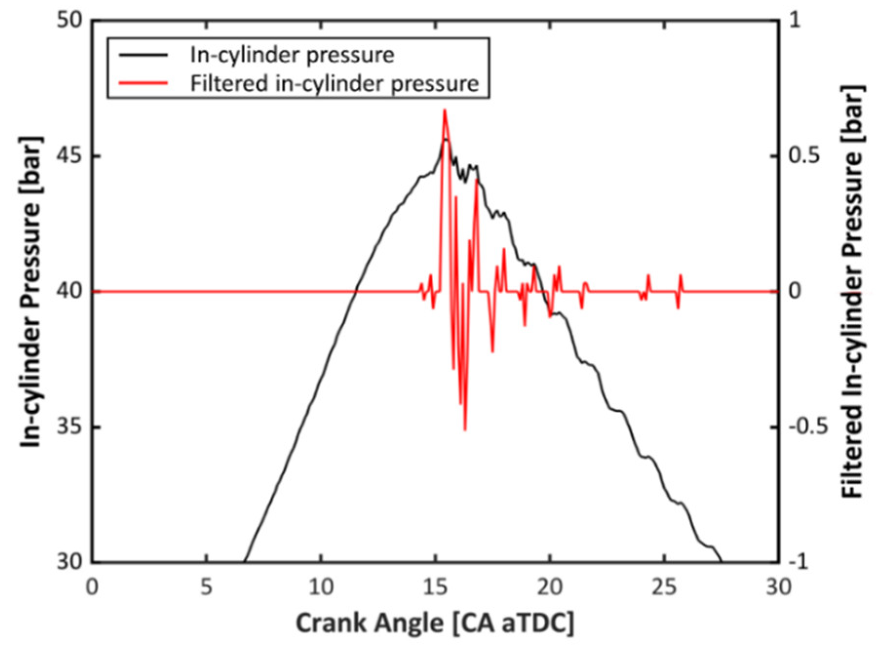
4.1. Signal Processing of In-Cylinder Pressure

Due to the sensitivity problem of in-cylinder pressure transducers, a large error can be made in the low-pressure region when analyzing an individual cycle. Therefore, a filtering method is required, especially for the intake period and exhaust period, as the values in the gas exchange process are broadly used to specify the state. However, a general filter such as Butterworth cannot be used due to the large phase-shifting problem, and a zero-phase filter is not adaptable either because there is no certain frequency.

Figure 7a shows the in-cylinder pressure trace near the intake valve closing (IVC) timing of an individual cycle. The black line indicates the unfiltered raw signal and shows an uneven behavior due to the aforementioned sensitivity issue. Even if a median filter (blue line) was applied, which is what many researchers have used, it still shows a picky trace. In the low-pressure region, the impact of this uneven trace is undoubtedly large due to the originally small value. In the example of Figure 7a, an almost 9% error was obtained in the pressure at the IVC timing, which corresponds to an approximately 30 K error in the temperature.

The reliable determination of the IVC pressure is one of the most important factors for the combustion analysis, as it is significantly influential to the whole process including compression and combustion, regardless of the analysis method. Therefore, a smooth filtering method was applied for the low-pressure region in this study. A 3rd-order and 151 frame-length Savitzky-Golay [41] smoothing filter was applied upon the median filter. The filtered signal is indicated with red lines in both Figure 7a,b, and it shows an improved performance in chasing the original signal.

On the other hand, when there is a knocking combustion, an error can exist during the heat release analysis because of the picky in-cylinder pressure trace. However, the previous smoothing technique causes an error in the high-pressure region and generally gives a lower pressure value. In addition, the in-cylinder pressure transducer is already capable of providing relatively reliable values in the high-pressure region. Thus, the combustion pressure signal was processed by using zero-phase filtering based on low-pass filter using the Kaiser window: 4 kHz of passband frequency, 5 kHz of stopband frequency, 1 dB of passband ripple and 65 dB of stopband attenuation. Zero-phase trimming was conducted using MATLAB ‘filtfilt’ function using specified design. Figure 8a shows the results: the defect of the smoothing method (red line) in the high-pressure region and the application of the zero-phase filter (blue line).

Thereby, two filtered signals were obtained: a smoothed pressure trace in the low-pressure region, as shown in Figure 7, and a zero-phase filtered pressure trace in the high-pressure region, as shown in Figure 8a. These two signals were then combined into one signal by calculating the internal division point with weight factors. This process was conducted using a hundred samples after the cylinder pressure exceeds 5 bar, where the error by the sensor is less than 0.5%. The weight was given from a hundred to zero for the smoothed signal and from zero to a hundred for the zero-phase filtered signal. An example of a merged signal is shown in Figure 8b. It is easily recognized that the merged trace (black line) follows the smoothed pressure in the low-pressure region and begins to follow the zero-phase filtered pressure in the higher-pressure region.

4.2. Residual Gas Fraction

Generally, combustion analysis begins with the ideal gas flow while the pressure and volume are given. Therefore, the total trapped mass or temperature is required for the characterization of the closed system state. The total trapped mass can be widely varied by changes in the operating conditions such as the valve overlap, ignition timing and throttle angle. The amounts of fuel and air can be easily obtained by measurement or relatively accurate models. Also for knocking studies, the ignition delay is one of the key parameters, and this is also influenced greatly by the temperature variation during the calculation.

4.2.1. One-Dimensional Simulation

In this study, an approach for the estimation of total trapped mass using a 0D residual gas fraction (RGF) model was studied. The engine was equipped with a dual VVT system, and thus a correct estimation was required. As it is not easy to measure the RGF accurately in massive operating conditions, a 1D simulation was adopted using the GT-POWER v2016 software to establish the 0D RGF model.

First, the 1D engine model was validated and optimized under motoring conditions. This process is very important since the RGF is mainly determined by the pressure gradients during the gas exchange process. The shapes of the air paths were optimized to considerably imitate the in-cylinder and intake manifold pressures. Figure 9 shows the matching result with the experimental data. A reliable model was achieved by validation under changes in the valve timings, engine speed, intake pressure and even hot/cold wall temperatures. Nevertheless, to minimize the complexity of this paper, a part of the results is shown in the figure. The simulation of the pressure oscillation in the intake manifold, which is one of the main targets in this procedure, was also well achieved.

After the flow characteristics were well reproduced, data matching was also conducted under firing conditions. The purpose of this procedure was to achieve the multiplier coefficients in conventional models related to the combustion process. The ‘SITurb’ combustion model was used for combustion and the ‘Woschni’ model was chosen for heat transfer in this study. The optimization was conducted based on the data of 14 experimental cases using the ‘Advanced Direct Optimizer’ in the software. The cases were chosen to include variations in the intake pressure, valve timings, engine speed and spark timings. The objective function of the optimization was set as the SSE (sum of squared errors) between the pressures obtained by simulation and experiment, and the window was set from 25 CA bTDC to 60 CA aTDC.

The optimized results are shown in Figure 10, and the parameters (multipliers) are listed in

Table 4. Multipliers for optimization.

Model	Multiplier	Optimized Value
Combustion (SITurb)	Flame Kernel Growth	1.167
	Turbulent Flame Speed	0.690
	Taylor Length Scale	0.703
Heat transfer (Woschni)	-	0.7

. The optimized models, SITurb (combustion) and Woschni (heat transfer), showed agreeable matching results with the experimental data. However, the multipliers obtained in this study are not universal, as they were only validated using the engine used in this study. In addition, there is an issue with the precision of the models [42]. Nonetheless, well-matched pressure profiles were achieved, so this point is beyond the scope of this study.

After the optimized engine model was achieved with validation under both motoring and firing conditions, a large quantity of validation data (a total of 1,200 cases) was collected using the DoE (design of experiment) process by changing the sweep parameters, as shown in

Table 5. Sweep parameters and ranges of the Dessign of Experiment (DoE) process.

Sweep Parameter	Range
Engine speed (rpm)	1500–3000
Spark timing (CA bTDC)	28–0
Intake pressure (bar)	0.2–1
Intake valve timing	0–40 adv.
Exhaust valve timing	0–30 rtd.
Total 1200 cases

.

In summary, for precise simulation, the flow characteristics and combustion behaviors were comprehensively matched using an optimization process based on experimental data. Sequentially, the DoE process was conducted to provide the back data to improve the 0D RGF model.

4.2.2. Improved RGF Model

Figure 11a,b show the results of the 0D RGF models proposed by Fox et al. [15] and Kale et al. [16], respectively. As previously described, validation data was provided by a 1D simulation. Genetic algorithm was used for the optimization (re-calibration) of the coefficients of each model. In the figures, the x-axis indicates the RGF values from the 1D simulation results, and the y-axis indicates the calculated values of the 0D RGF model. Kale’s model shows acceptable accuracy, while Fox’s model shows poorer accuracy. However, there were underestimated and overestimated data points, as can easily be observed in Figure 11b. Detailed explanations of the two models are provided in the references and thus skipped in this paper.

An attempt was made to improve the accuracy of the conventional RGF model in this study. As previously shown, Kale’s model showed great potential. However, due to the empirical and simplified form of the model, it occasionally gave negative RGF values under conditions with high volumetric efficiency. In addition, it was found that the sensitivity of the volumetric efficiency was undervalued. Therefore, an adjustment was made to change the impact of the volumetric efficiency from linear to exponential. The changed expressions of the OF are as follows:

$$O{F}_{s.IVC}=a·O{F}_{C, IN}+b·O{F}_{C, EX}+{\eta }_v{}^c+d$$

(8)

$$O{F}_{ns.IVC}=e·\left(O{F}_{C.IN}-O{F}_{C.EX}\right)+{\eta }_v{}^f$$

(9)

Figure 11c shows the result of the improved RGF model. The R-squared value was increased to 0.883, while it was 0.289 in Fox’s model and 0.763 in Kale’s model. With a further consideration of the volumetric efficiency, the data points located above and below the identity line have been moved. However, an inexactitude was observed, especially in the low-RGF region, and the model still requires many tuning coefficients. Therefore, further study is still required.

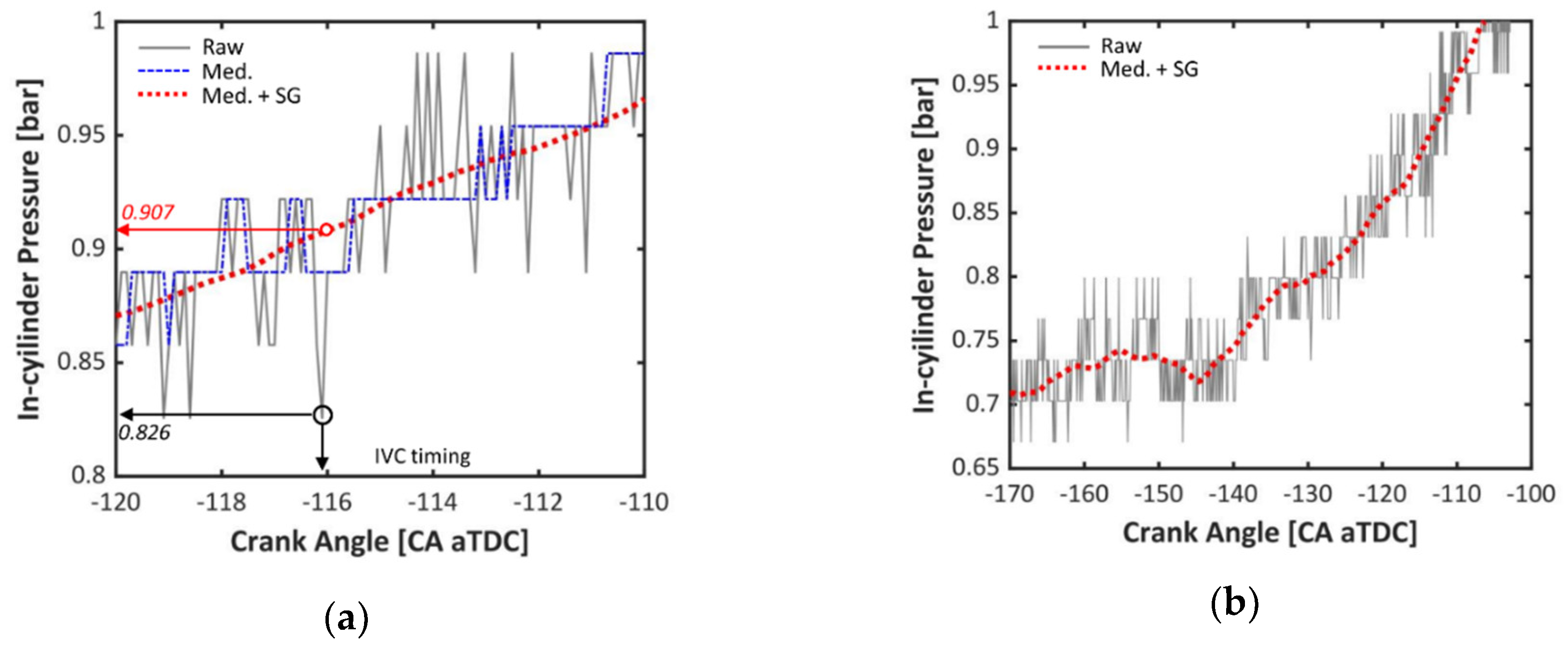
4.3. Characterization of IVC State

During the experiment, the in-cylinder pressure is given by measurement, and the volume can be simply calculated from the geometry. Assuming that there is no blow-by, the state of the IVC can be determined by the ideal gas law. In the experimental test environment, the air input mass can be obtained by considering the air-fuel ratio (or lambda) or by direct measurement. However, as was previously discussed, the proportion of residual gas is important not only for the characterization of the state of the closed system but also for the gas property inside the chamber. Based on the previously achieved RGF model and using the error-minimized pressure curve, the temperature at the IVC can be obtained as Equation (10) below:

$$T_{IVC}=\frac{P_{IVC}{V}_{IVC}}{\left(n_{fuel}+n_{air}+n_{residual}\right)R}$$

(10)

4.4. Unburned Gas Temperature

For the further understanding of the knock phenomena, the condition of the unburned gas has to be investigated because knock occurs in the unburned end-gas region during the combustion process. Several parameters are required: the pressure, temperature, and mixture properties such as composition. Under test conditions, the pressure is easily obtained using an in-cylinder pressure transducer and data acquisition system. In addition, since the pressure wave travels at sonic speed, it is reasonable to assume that the pressure of the unburned gas region is the same as the measured in-cylinder pressure. However, it is not simple to measure the in-cylinder temperature due to the harsh in-cylinder conditions. Therefore, estimations by modeling are commonly used. In this section, a 0D analysis approach with experimental data is interpreted.

During the combustion process, because the flame is initiated by the spark plug in the spark-ignited engine, the gas mixture is divided into two zones: burned and unburned. While the pressure is the same for both zones, the temperature and mixture properties are apparently different. Therefore, a two-zone based approach is needed. There are two general approaches to the calculation of the unburned gas temperature: bulk and core [43]. The estimation method of the heat transfer amount has an impact on the calculation approach of the bulk temperature of the unburned gas.

The conventional two-zone approach [1,43,44,45] is that considering that the crevice effect can be neglected, mass and energy conservation and the perfect ideal gas law are applied to both burned and unburned zones. A calculation method by Catania et al. [44] for the unburned temperature is shown in Equation (11), where $T_u$ is the temperature of the bulk unburned end-gas, $P$ is the pressure, which is obtained by measurement, $c_{p,u}$ is the specific heat at constant pressure, $m$ is the trapped total mass, $R_{s,u}$ is specific ideal gas constant and $q_u$ is the heat transfer rate of unburned gas to the wall:

$$-q_u{A}_{u}dt=\left(1-x_b\right)m(c_{p,u}d{T}_u-R_{s,u}{T}_u\frac{dP}{P})$$

(11)

Considering that the heat transfer is zero, an expression for core gas temperature can be obtained as Equation (12). By assuming that heat transfer occurs between the thermal boundary layer and walls in the unburned gas region, the core gas of the unburned mixture can be considered to be adiabatically compressed by the pressure, and the obtained pressure value is already decreased by the actual heat transfer. Autoignition can be thought to possibly occur in the core gas, where the highest temperature exists in the unburned end gas:

$$T=T_{IVC}{\left(\frac{P}{P_{IVC}}\right)}^{1-\frac{1}{\gamma }}$$

(12)

Calculation was conducted from IVC to exhaust valve opening (EVO). Cantera 2.4.0 [46] with the detailed PRF mechanism of Lawrence Livermore National Laboratory (LLNL) was used for the calculation of the gas properties at every state. The surrogate fuel was simply set to have an RON of 91.5 since the gas property is not sensitive to the variation of the fuel due to its low molar fraction. The initial gas composition was defined as a mixture of fuel, intake air and residual gas. For the composition of the residual gas, the emission test result was used.

For the precise calculation of the specific heat and temperature, an iteration method was adopted. The initial unburned gas temperature was assumed to be the same as that of the IVC, and the single-zone based gamma from the previous section was used for the first iteration. The temperature and specific heat value were calculated, and the iteration stopped when the RMSE of the specific heat ratio value was under 1 × 10⁻⁴ between the n^th and n−1^th iterations from IVC to EVO. It was observed that fewer than five iterations were normally sufficient.

5. Knock Prediction Model

One of the main purposes of this study is to predict knock occurrence. Because an instantaneous cycle analysis was established, proper assumptions and the estimation of the in-cylinder pressure will facilitate an on-board knock control in the transient condition. In this study, as the 0D RGF model has been improved, the calculation of the gas composition was facilitated. In terms of the chemical reaction rate shown in Equation (13), where $\left[Fuel\right]$ and $\left[O_2\right]$ are the molar fractions of the fuel and oxygen respectively, a simplified correlation of the ignition delay can be obtained as Equation (14) [47,48], neglecting the NTC (negative temperature coefficient) behavior. This correlation of the 0D ignition delay is physically based on a simplified chemical mechanism, and thus the actual behavior is different. However, following the main purpose of this study, the feasibility of the knock prediction was tested based on an instantaneous cycle analysis:

$$r=A{\left[Fuel\right]}^m{\left[O_2\right]}^{n}exp\left(-\frac{E_a}{RT}\right)$$

(13)

$$\tau =C_1{\left(\frac{P}{T}\right)}^{-C_2}{\left[Fuel\right]}^{-C_3}{\left[O_2\right]}^{-C_4}exp\left(\frac{C_5}{T}\right)$$

(14)

Using previously interpreted methods, the individual knocking cycles were analyzed in a wide range of experimental conditions including changes in the intake pressure, valve timing and engine speed. The genetic algorithm was applied for the optimization, adjusting the five coefficients to minimize the RMSE between the 0D model-predicted KO and experimental KO (obtained using the aforementioned smart KO model). The multiplier for crossover was 0.7, for mutation was 0.3 and the generation limit was set to 25. Usually, the minimum objective function was achieved before the 20^th generation during the optimization. As a result, Equation (15) was achieved:

$$\tau =5.745\times {10}^{-8}{\left(\frac{P}{T}\right)}^{-1.966}{\left[Fuel\right]}^{-0.548}{\left[O_2\right]}^{-0.415}exp\left(\frac{7094}{T}\right)$$

(15)

Figure 12 shows the validation result of the prediction model in 16,454 knocking cycles. Total 21 experimental cases (63,000 cycles) were tested with 3,000 cycles in each, in a wide range of experimental conditions, as shown on the right side in the figure. The x-axis indicates the KO evaluated from the smart knock onset model, and the y-axis indicates the predicted KO by the 0D ignition delay and Livengood-Wu integral.

A satisfactory correlation (RMSE = 1.28) was achieved in spite of not using average values in an engine equipped with dual phasing camshafts. Studies on knock prediction models rely on the calculation starting from the average in-cylinder condition of the IVC timing. Usually, this initial condition is obtained using 1D simulation, or, even if the study utilized the instantaneous value, the model was not universal under all conditions. The achievement of this study is not only the establishment of a knock prediction model but also its availability for the utilization of an individual cycle analysis. This implies that there is a sufficient possibility of a reliable model for knock prediction in the transient condition. It is expected that pressure value predicted by the manifold absolute pressure sensor can be used for actual engine application.

Figure 13 depicts the results by the different methodologies. The predicted model based on the normal cycle analysis is shown in Figure 13a, and the result based on the aforementioned cyclic analysis is shown in Figure 13b. For the calculation of the case in Figure 13a, no filter was applied to the in-cylinder pressure, and the specific heat ratio was fixed to 1.32. However, the smart KO model was still utilized in this case. For clarity, only a few cases with a large valve overlap cases are plotted in both figures. A better correlation was apparently achieved by using the analysis method in this paper. This is mainly attributed to the improved characterization of the IVC timing.

Figure 14a shows the result of a previous knock prediction model that was newly calibrated using experimental data and the analysis method of this study. It shows a nice correlation, but due to the impact of the residual gas fraction, cases with a small valve overlap (plotted with red dots) showed slightly biased behaviors. The calibration process also includes extreme cases with a negative valve overlap and large valve overlap; the coefficient of the ignition delay correlation could not fully include the small valve overlap condition. On the other hand, in the developed model, as the RGF was reasonably predicted and included during the gas temperature calculation, the impacts of the valve timing and overlap were sufficiently reflected with the suggested correlation. The KOs in the positive valve overlap cases are located on the left bottom corner of both figures where the region of the KO is advanced. This is mainly attributed to the impact of the hot residual gas, which deteriorates the knock resistance. Therefore, an NVO strategy was applied in the high-load condition utilizing a retarded ignition timing. A better performance was achieved, shown as a lower RMSE (1.42 → 1.28) in the figures.

6. An Insight into the Knock Intensity

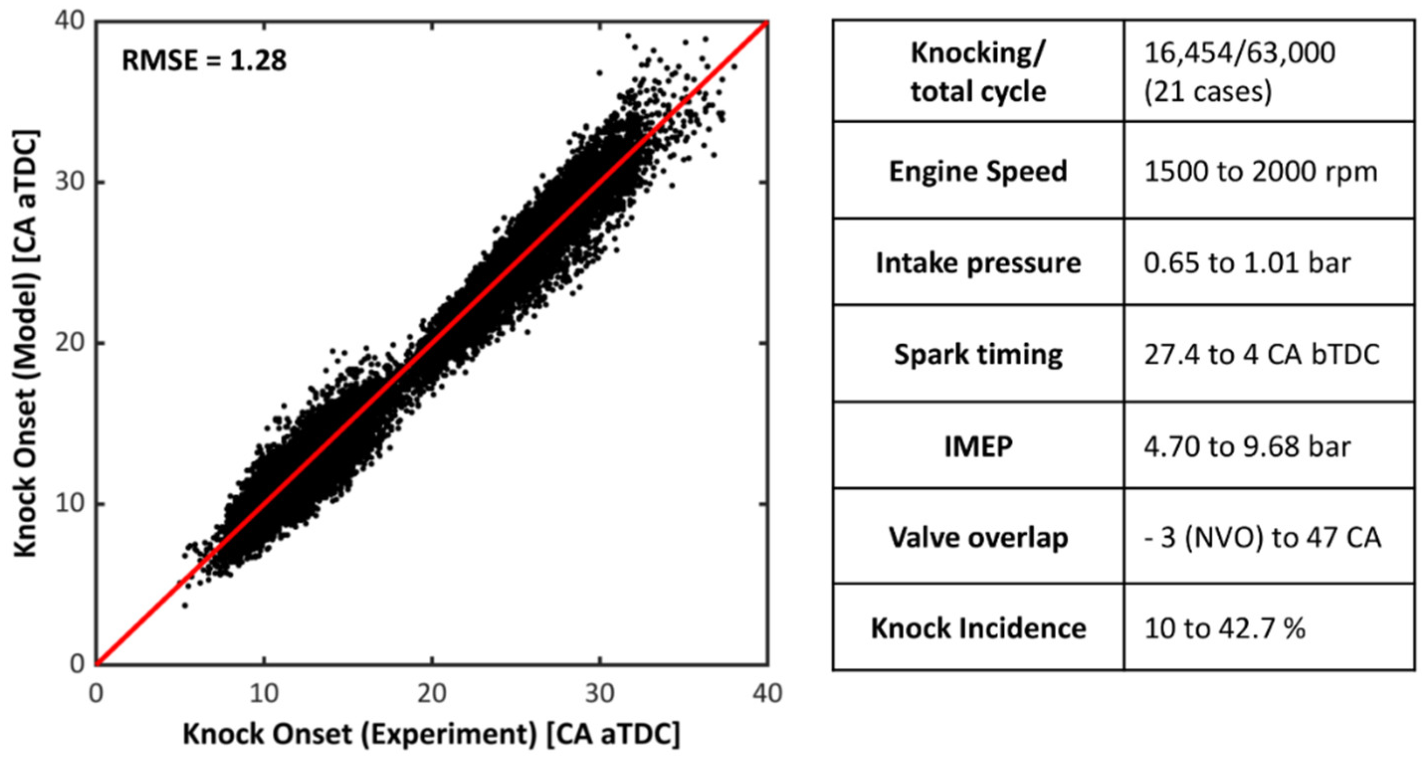
6.1. Experimental Result

Figure 15 shows a result of an individual cycle analysis. The engine speed was 1500 rpm, the intake pressure was 0.95 bar, the spark timing was 11.5 CA bTDC and the load was 7.47 bar of IMEP. A total of 10k consecutive cycles were analyzed in this operating condition. Considering that the intensity of autoignition can be represented with the MAPO value in a cycle, cycles with over 1 bar of MAPO are indicated with red dots, and cycles with under 0.5 bar MAPO are indicated with black dots in the figures. Nevertheless, there are various methods for the intensity calculation [38].

Figure 15a shows the in-cylinder pressure at the KO as a function of the burn duration. A clear negative linearity between the two parameters was observed. When the burn duration is short, it can reach a higher pressure earlier than a slow burn cycle at the same time, which results in a shorter ignition delay until the KO. Slow burn cycles need a longer ignition delay time, and therefore a lower pressure was obtained at the KO. An interesting thing was discovered that the overall MAPO is higher with a faster combustion speed; the red-dotted cluster is located at the upper left side of the black-dotted data points. This implies that a shorter burn duration led to a higher knock intensity. This classification was facilitated by using the previously described individual cycle analysis.

Figure 15b displays the relationship between in-cylinder pressure at the KO and mass fraction burned (MFB). In the figure, a lower MFB value was observed at a higher MAPO considering that the red cluster is located at the upper left region compared to the black points. This indicates that the larger mass of unburned gas provoked a stronger autoignition that developed into the knock. Additionally, it is shown that the in-cylinder pressure was higher when there is a larger unburned gas fraction (smaller MFB).

Figure 15c shows the pressure and temperature at the KO. A higher knock intensity was generally achieved with a higher pressure and temperature. As the knock intensity is mainly attributed to the pressure and the temperature gradient in the hot spot [7], the relationship between the MAPO and temperature gradient was investigated and not apparently observed due to its stochastic behavior, while it was assumed that the temperature gradient was generally proportional to the difference between the core and bulk gas temperatures. However, there was a relationship between the knock intensity and the amount of unburned gas. Therefore, it is thought that the higher pressure at the KO is a result of fast combustion which shortens the ignition delay, leading to a lower MFB at the KO, and this results in a higher knock intensity.

6.2. Model-Based Approach

As a reliable correlation of the 0D ignition delay was achieved previously, a model-based approach was attempted to understand this phenomenon. In Figure 16, actual MFB curves of the total cycle data are indicated as gray lines, and the cyclic variation can be easily noted. Using this MFB curve, the autoignition timings are plotted with dots. In the same manner as in the previous result, the KO results are plotted with two colors according to the measured MAPO values.

Two things should be noted from the result. First, as the measurement data contains the stochastic behavior of the knock phenomena, there are fast burn cycles with a zero knock intensity, and the opposite exists as well, slow burn cycles with a high MAPO value. Following the autoignition timing by using the previous empirical correlation, the autoignition timings are still shown in the slow burn cycles in the figure because the Livengood-Wu correlation only gives the ignition timing. However, as it is shown in Figure 15b that little autoignition occurred after MFB80, it can be considered that it cannot develop into knock.

Second, it is shown that a faster combustion leads to a higher knock intensity by increasing the unburned mass fraction at the KO, under steady-state operating condition. Faster combustion has been an efficient method to mitigate the knocking combustion to date, but it was shown that increasing the combustion speed might be helpful to mitigate the occurrence of knock (incidence), whereas there was a possibility of an increase in the knock intensity. This behavior is mainly attributed to the interaction between the in-cylinder condition and air-fuel mixture that determines the ignition delay. This elucidates that in fast combustion, the decrease in ignition delay followed by pressure increase is more sensitive than the decrease of the unburned gas amount, so this implies that designing combustion speed is required for higher knock resistance.

7. Conclusions

The present work introduces a systematic methodology to analyze the in-cylinder pressure in individual cycled knocking combustion with several improvements for higher accuracy. The objective of the proposed methodology relies on not only providing a high-quality combustion analysis but also facilitating a model-based knock control under transient conditions in the future. For this objective, several attempts were made.

Because the correct determination of the knock onset is significantly important for individual cycle analysis, a smart knock onset model was developed using a supervised deep learning method. To obtain the best model for applicability, a parametric optimization was conducted by varying the number of hidden layers, epoch number and learning rate. As a result, the highest accuracy was achieved compared to other models, and no cycle loss was found during the analysis.

As conventional filters cannot be utilized due to the limitations of the pressure transducer and signal distortion problem, proper filtering methods were proposed in each of the low-pressure region (3^rd-order, 151 frame-length Savitzky-Golay smoothing) and high-pressure region (zero-phase filtering with Kaiser window). In addition, a merging skill adopting weighting factors was introduced.

To characterize the initial state of the closed system, the estimation of the total trapped mass is also important. Thus, a 0D RGF model was enhanced from a previous model (Kale’s). The result was validated in big data based on a sophisticated 1D simulation model, and it showed an improved correlation (R² = 0.883). Consequently, reasonable estimation could be made for the state at the IVC timing with a further consideration of the volumetric efficiency.

A knock prediction model with a satisfactory correlation (RMSE of 1.28 of in 16,454 cycles) was achieved by simply assuming a constant-speed chemical reaction under various operating conditions including aggressive changes in the cam timings using a dual VVT system. It showed a feasibility of utilizing the individual cycle data, which may allow on-board knock control in a transient condition in the future, which is the author’s future study.

Using the proposed methodologies for the analysis, it was shown that a faster combustion cycle had a possibility of a higher knock intensity in a steady-state operating condition, because the amount of unburned mass is larger in spite of the reduced combustion duration.

References

1. Heywood, J.B. Internal Combustion Engine Fundamentals; McGraw-Hill: New York, NY, USA, 1988. [Google Scholar]
2. Zhen, X.; Wang, Y.; Xu, S.; Zhu, Y.; Tao, C.; Xu, T.; Song, M. The engine knock analysis–An overview. Appl. Energy 2012, 92, 628–636. [Google Scholar] [CrossRef]
3. Wang, Z.; Liu, H.; Reitz, R.D. Knocking combustion in spark-ignition engines. Prog. Energy Combust. Sci. 2017, 61, 78–112. [Google Scholar] [CrossRef]
4. Nates, R.; Yates, A. Knock Damage Mechanisms in Spark-Ignition Engines. In SAE Technical Paper 942064; SAE International: Warrendale, PA, USA; Troy, MI, USA, 1994. [Google Scholar]
5. Fitton, J.; Nates, R. Knock Erosion in Spark-ignition Engines. In SAE Technical Paper 962102; SAE International: Warrendale, PA, USA; Troy, MI, USA, 1996. [Google Scholar]
6. Kalghatgi, G.; Algunaibet, I.; Morganti, K. On knock intensity and superknock in SI engines. SAE Int. J. Engines 2017, 10, 1051–1063. [Google Scholar] [CrossRef]
7. Kalghatgi, G.; Morganti, K.; Algunaibet, I. Some Insights on the Stochastic Nature of Knock and the Evolution of Hot Spots in the End-Gas During the Engine Cycle from Experimental Measurements of Knock Onset and Knock Intensity. In SAE Technical Paper 2017-01-2233; SAE International: Warrendale, PA, USA; Troy, MI, USA, 2017. [Google Scholar]
8. Worret, R.; Bernhardt, S.; Schwarz, F.; Spicher, U. Application of Different Cylinder Pressure Based Knock Detection Methods in Spark Ignition Engines. In SAE Technical Paper 2002-01-1668; SAE International: Warrendale, PA, USA; Troy, MI, USA, 2002. [Google Scholar]
9. Lee, J.-H.; Hwang, S.-H.; Lim, J.-S.; Jeon, D.-C.; Cho, Y.-S. A New Knock-Detection Method using Cylinder Pressure, Block Vibration and Sound Pressure Signals from a SI Engine. In SAE Technical Paper 981436; SAE International: Warrendale, PA, USA; Troy, MI, USA, 1998. [Google Scholar]
10. Shahlari, A.J.; Ghandhi, J.B. A Comparison of Engine Knock Metrics. In SAE Technical Paper 2012-32-0037; SAE International: Warrendale, PA, USA; Troy, MI, USA, 2012. [Google Scholar]
11. Kim, K.S. Study of Engine Knock Using A Monte Carlo Method; The University of Wisconsin-Madison: Madison, WI, USA, 2015. [Google Scholar]
12. Yun, H.; Mirsky, W. Schlieren-Streak Measurements of Instantaneous Exhaust Gas Velocities from a Spark-Ignition Engine. In SAE Technical Paper 7410252; SAE International: Warrendale, PA, USA; Troy, MI, USA, 1974. [Google Scholar]
13. Guardiola, C.; Triantopoulos, V.; Bares, P.; Bohac, S.; Stefanopoulou, A. Simultaneous estimation of intake and residual mass using in-cylinder pressure in an engine with negative valve overlap. IFAC-PapersOnLine 2016, 49, 461–468. [Google Scholar] [CrossRef]
14. Fitzgerald, R.P.; Steeper, R.; Snyder, J.; Hanson, R.; Hessel, R. Determination of Cycle Temperatures and Residual Gas Fraction for HCCI Negative Valve Overlap Operation. SAE Int. J. Engines 2010, 3, 124–141. [Google Scholar] [CrossRef]
15. Fox, J.W.; Cheng, W.K.; Heywood, J.B. A Model for Predicting Residual Gas Fraction in Spark-Ignition Engines; SAE International: Warrendale, PA, USA; Troy, MI, USA, 1993. [Google Scholar]
16. Kale, V.; Yeliana, Y.; Worm, J.; Naber, J. Development of an Improved Residuals Estimation Model for Dual Independent Cam Phasing Spark-Ignition Engines; SAE International: Warrendale, PA, USA; Troy, MI, USA, 2013. [Google Scholar]
17. Chen, L.; Li, T.; Yin, T.; Zheng, B. A predictive model for knock onset in spark-ignition engines with cooled EGR. Energy Convers. Manag. 2014, 87, 946–955. [Google Scholar] [CrossRef]
18. Moses, E.; Yarin, A.L.; Bar-Yoseph, P. On knocking prediction in spark ignition engines. Combust. Flame 1995, 101, 239–261. [Google Scholar] [CrossRef]
19. Sazhin, S.; Sazhina, E.; Heikal, M.; Marooney, C.; Mikhalovsky, S. The Shell autoignition model: A new mathematical formulation. Combust. Flame 1999, 117, 529–540. [Google Scholar] [CrossRef]
20. Sazhina, E.; Sazhin, S.; Heikal, M.; Marooney, C. The Shell autoignition model: Applications to gasoline and diesel fuels. Fuel 1999, 78, 389–401. [Google Scholar] [CrossRef]
21. Livengood, J.; Wu, P. Correlation of autoignition phenomena in internal combustion engines and rapid compression machines. Symposium (Int.) Combust. 1955, 5, 347–356. [Google Scholar] [CrossRef]
22. Douaud, A.; Eyzat, P. Four-Octane-Number Method for Predicting the Anti-Knock Behavior of Fuels and Engines. In SAE Technical Paper 780080; SAE International: Warrendale, PA, USA; Troy, MI, USA, 1978. [Google Scholar]
23. Mittal, V.; Revier, B.M.; Heywood, J.B. Phenomena that Determine Knock Onset in Spark-Ignition Engines. In SAE Technical Paper 2007-01-0007; SAE International: Warrendale, PA, USA; Troy, MI, USA, 2007. [Google Scholar]
24. Kasseris, E.; Heywood, J.B. Charge cooling effects on knock limits in si di engines using gasoline/ethanol blends: Part 2-effective octane numbers. SAE Int. J. Fuels Lubr. 2012, 5, 844–854. [Google Scholar] [CrossRef]
25. Siokos, K.; He, Z.; Prucka, R. Assessment of Model-Based Knock Prediction Methods for Spark-Ignition Engines. In SAE Technical Paper 2017-01-0791; SAE International: Warrendale, PA, USA; Troy, MI, USA, 2017. [Google Scholar]
26. Burluka, A.; Liu, K.; Sheppard, C.; Smallbone, A.; Woolley, R. The Influence of Simulated Residual and NO Concentrations on Knock Onset for PRFs and Gasolines. In SAE Technical Paper 2004-01-2998; SAE International: Warrendale, PA, USA; Troy, MI, USA, 2004. [Google Scholar]
27. Wayne, W.S.; Clark, N.N.; Atkinson, C.M. Numerical Prediction of Knock in a Bi-Fuel Engine. In SAE Technical Paper 982533; SAE International: Warrendale, PA, USA; Troy, MI, USA, 1998. [Google Scholar]
28. Pipitone, E.; Beccari, S. Calibration of a knock prediction model for the combustion of gasoline-natural gas mixtures. In Proceedings of the ASME 2009 Internal Combustion Engine Division Fall Technical Conference, Lucerne, Switzerland, 27–30 September 2009; pp. 191–197. [Google Scholar]
29. Hoepke, B.; Jannsen, S.; Kasseris, E.; Cheng, W.K. EGR effects on boosted SI engine operation and knock integral correlation. SAE Int. J. Engines 2012, 5, 547–559. [Google Scholar] [CrossRef]
30. McKenzie, J.; Cheng, W.K. Ignition Delay Correlation for Engine Operating with Lean and with Rich Fuel-Air Mixtures. In SAE Technical Paper 2016-01-0699; SAE International: Warrendale, PA, USA; Troy, MI, USA, 2016. [Google Scholar]
31. Asif, M.; Giles, K.; Lewis, A.; Akehurst, S.; Turner, N. Influence of Coolant Temperature and Flow Rate, and Air Flow on Knock Performance of a Downsized, Highly Boosted, Direct-Injection Spark Ignition Engine. In SAE Technical Paper 2017-01-0664; SAE International: Warrendale, PA, USA; Troy, MI, USA, 2017. [Google Scholar]
32. Brunt, M.F.; Pond, C.R.; Biundo, J. Gasoline Engine Knock Analysis using Cylinder Pressure Data. In SAE Technical Paper 980896; SAE International: Warrendale, PA, USA; Troy, MI, USA, 1998. [Google Scholar]
33. Bertola, A.; Stadler, J.; Walter, T.; Wolfer, P.; Gossweiler, C.; Rothe, M. Pressure indication during knocking conditions. In Proceedings of the Seventh International AVL Symposium on Internal Combustion Diagnostics, Baden-Baden, Germany, 18–19 May 2006. [Google Scholar]
34. Lancaster, D.R.; Krieger, R.B.; Lienesch, J.H. Measurement and Analysis of Engine Pressure Data. In SAE Technical Paper 750028; SAE International: Warrendale, PA, USA; Troy, MI, USA, 1975. [Google Scholar]
35. Brunt, M.F.; Lucas, G.G. The Effect of Crank Angle Resolution on Cylinder Pressure Analysis. In SAE Technical Paper 910041; SAE International: Warrendale, PA, USA; Troy, MI, USA, 1991. [Google Scholar]
36. Millo, F.; Ferraro, C.V. Knock in S.I. Engines: A Comparison between Different Techniques for Detection and Control. In SAE Technical Paper 982477; SAE International: Warrendale, PA, USA; Troy, MI, USA, 1998. [Google Scholar]
37. Sjöberg, M.; Vuilleumier, D.; Yokoo, N.; Nakata, K. Effects of Gasoline Composition and Octane Sensitivity on the Response of DISI Engine Knock to Variations of Fuel-Air Equivalence Ratio. In Proceedings of the International Symposium on Diagnostics and Modeling of Combustion in Internal Combustion Engines, Okayapa, Japan, 25–28 July 2017; p. B307. [Google Scholar]
38. Borg, J.M.; Alkidas, A.C. Cylinder-pressure-based methods for sensing spark-ignition engine knock. Int. J. Veh. Des. 2007, 45, 222–241. [Google Scholar] [CrossRef]
39. McCulloch, W.S.; Pitts, W. A logical calculus of the ideas immanent in nervous activity. J. Bull. Math. Biophys. 1943, 5, 115–133. [Google Scholar] [CrossRef]
40. Rumelhart, D.E.; Mcclelland, J.L. Parallel Distributed Processing: Explorations in the Microstructure of Cognition. Volume 1. Foundations; MIT Press: Cambridge, MA, USA, 1986; p. 564. [Google Scholar]
41. Savitzky, A.; Golay, M.J. Smoothing and differentiation of data by simplified least squares procedures. Anal. Chem. 1964, 36, 1627–1639. [Google Scholar] [CrossRef]
42. Kim, N.; Ko, I.; Min, K. Development of a zero-dimensional turbulence model for a spark ignition engine. Int. J. Engine Res. 2018. [Google Scholar] [CrossRef]
43. Ferguson, C.R.; Green, R.M.; Lucht, R.P. Unburned Gas Temperatures in an Internal Combustion Engine. II:Heat Release Computations AU—Ferguson, Colin R. Combust. Sci. Technol. 1987, 55, 63–81. [Google Scholar] [CrossRef]
44. Catania, A.; Misul, D.; Mittica, A.; Spessa, E. A refined two-zone heat release model for combustion analysis in SI engines. JSME Int. J. Ser. B Fluids Thermal Eng. 2003, 46, 75–85. [Google Scholar] [CrossRef]
45. Ferguson, C.R.; Kirkpatrick, A.T. Internal Combustion Engines: Applied Thermosciences; John Wiley & Sons: Hoboken, NJ, USA, 1986. [Google Scholar]
46. Goodwin, D.G.; Speth, R.L.; Moffat, H.K.; Weer, B.W. Cantera: An Object-Oriented Software Toolkit for Chemical Kinetics, Thermodynamics, and Transport Processes. Available online: http://www.cantera.org (accessed on 7 February 2019).
47. Ryan, T.W.; Callahan, T.J. Engine and Constant Volume Bomb Studies of Diesel ignition and Combustion; SAE International: Warrendale, PA, USA; Troy, MI, USA, 1988. [Google Scholar]
48. Finesso, R.; Spessa, E. Ignition delay prediction of multiple injections in diesel engines. Fuel 2014, 119, 170–190. [Google Scholar] [CrossRef]
Figure 1. Engine test configuration.
Energies 12 00844 g001
Figure 2. Filtering of in-cylinder pressure signal under knocking condition. aTDC: After top-dead center.
Energies 12 00844 g002
Figure 3. Error in determination of KO by TVE method: (a) heavy knock condition; (b) weak knock condition. KO: Knock-onset; TVE: Threshold value exceeded.
Energies 12 00844 g003
Figure 4. Structure of deep learning and its input and output.
Energies 12 00844 g004
Figure 5. Parametric optimization of KO model using deep learning.
Energies 12 00844 g005
Figure 6. Various methods for KO determination: (a) TVE; (b) Kim; (c) Shahlari; (d) Smart KO model.
Energies 12 00844 g006
Figure 7. Filtering of in-cylinder pressure in low-pressure region: (a) Median and Savitzky-Golay filtering; (b) Overall shape of the pressure signal with newly applied filter.
Energies 12 00844 g007
Figure 8. Post-processing of in-cylinder pressure signal: (a) zero-phase filtering in high-pressure region; (b) signal merging.
Energies 12 00844 g008
Figure 9. One-dimensional (1D) simulation results in motoring conditions: (a) 1500 rpm, WOT, INCam 30 CA advanced; (b) 2000 rpm, WOT, INCam 30 CA advanced; (c) 2000 rpm, WOT, INCam fully retarded.
Energies 12 00844 g009
Figure 10. 1D simulation results in various firing conditions.
Energies 12 00844 g010
Figure 11. Matching results of conventional models: (a) Fox’s 0D RGF model; (b) Kale’s 0D RGF model; (c) Improved model.
Energies 12 00844 g011
Figure 12. Knock prediction model with individual cycle data.
Energies 12 00844 g012
Figure 13. Results of knock prediction modeling: (a) methodology not applied; (b) methodology applied.
Energies 12 00844 g013
Figure 14. Results of knock prediction models: (a) previous studies; (b) present.
Energies 12 00844 g014
Figure 15. Result of individual cycle analysis: (a) Pcyl@KO and MFB; (b) Pcyl@KO and MFB; (c) Pcyl@KO and unburned gas temperature. MFB: mass fraction burned.
Energies 12 00844 g015
Figure 16. Knock onset, intensity and mass fraction burned.
Energies 12 00844 g016