Sliding Mode Output Regulation for a Boost Power Converter †


1
CONACYT–Advanced Studies and Research Center (CINVESTAV), National Polytechnic Institute (IPN), Guadalajara Campus, Zapopan 45015, Mexico
2
Advanced Studies and Research Center (CINVESTAV), National Polytechnic Institute (IPN), Guadalajara Campus, Zapopan 45015, Mexico
3
Ceti Unidad Colomos, Calle Nueva Escocia 1885, Providencia 5a Sección, Guadalajara 44638, Mexico
*
Author to whom correspondence should be addressed.
†
This paper is an extended version of our paper published in CCE 2012, Mexico city, Mexico, 26–28 September 2012.
Energies 2019, 12(5), 879; https://doi.org/10.3390/en12050879
Submission received: 21 November 2018
/
Revised: 23 January 2019
/
Accepted: 21 February 2019
/
Published: 6 March 2019
(This article belongs to the Special Issue Sliding Mode Control of Power Converters in Renewable Energy Systems)
Abstract
:This work deals with the novel application of the sliding mode (discontinuous) output regulation theory to a nonlinear electrical circuit, the so-called boost power converter. This theory has excelled due to the fact that trajectory tracking plays a central role. The control of a boost power converter for the output tracking of a DC biased sinusoidal signal is a challenging problem for control engineers. The main difficulties are the computation of a proper reference signal for the inductor current, and the stabilization of the inductor current dynamics or to guarantee the correct output tracking of the capacitor voltage. With the application of the discontinuous output regulation these problems are solved in this work. Simulations and real time experiments were carried out with an unknown variation of the DC input voltage, where the good output tracking of the capacitor voltage was verified along with the stabilization of the inductor current. The discontinuous output regulation theory has proven to be a suitable tool in the output tracking for the boost power converter.
1. Introduction
Switched mode DC-DC power converters [1], are mainly used as constant current sources for LEDs, industry lighting, mobile phones, and photovoltaic systems [2,3]. Among the well known DC-DC converter topologies as buck, boost, buck-boost and cúk converters, the last three mentioned topologies result in being nonminimum-phase when directly controlling the output capacitor voltage variable [4]. Therefore, these topologies constitute a challenging area in the nonlinear control design point of view, attracting attention from researchers. Hence, several control techniques, either linear or nonlinear, to regulate these converters have been proposed such as input-output feedback linearization [5], boundary-conduction mode [6], linear designs [7], sliding mode control [8,9,10], current-mode-control [11], artificial neural networks [12], fuzzy logic control [13], passivity-based control [14], discontinuous conduction mode [15,16], among others.
With respect to the DC-AC power conversion using the traditional switched DC-DC power converter topologies, this has also attracted attention from researchers. In particular, in the work presented in [17], two closed-loop boost power converters were proposed for the DC-AC power conversion problem. One boost converter was controlled for the tracking of a DC biased sinusoidal signal, producing at the output a unipolar voltage. The other boost converter was controlled to track at the output the same signal, but with a phase value of 180°. The load was connected differentially across the converters. Thus, whereas a DC bias appears at each end of the load with respect to ground, the differential DC voltage over the load is zero, obtaining an AC voltage across the load. Two main advantages are noted in this work: the peak value of the AC voltage is larger than the DC input voltage due to the voltage raise property of the boost power converter, the other advantage is the possibility of harmonic reduction that will depend on the accuracy of the controllers for the generation of DC biased sinusoidal voltages at the outputs of each boost converter. Also, in the work [18], a cascade control strategy based on the sliding mode control was presented for the boost inverter. An analytical approach to describe the sliding mode motion was presented, and the generation of a sinusoidal signal with grid frequency and very low distortion was experimentally verified.
After the work presented in [17], the control design for the output tracking of a DC biased sinusoidal signal for a single boost power converter, became popular among researchers, where two control methods are distinguished: the direct and indirect methods. These control methods are characterized by the following problems:
- In the direct control method, the output capacitor voltage is directly controlled for tracking a proposed reference signal, yielding to a nonminimum-phase system, i.e., the residual inductor current dynamics is unstable. For a given capacitor voltage reference signal, the computation of a proper reference signal for the inductor current is a difficult task;
- In the indirect control method, the inductor current is directly controlled for tracking a proposed reference signal, yielding to a minimum-phase system, i.e., the residual capacitor voltage dynamics is stable, but the proposal of the inductor current reference signal that yields the desired behaviour at the output capacitor voltage is also a difficult task.
In the effort to solve these problems, one can find in the literature several works as the one in [8] where the flatness property of the system is exploited with an indirect control approach. This work is characterized by determining the inductor current in an iteratively fashion, and by a residual dynamics of the output capacitor voltage where its convergence to its desired reference signal results difficult to be demonstrated. In [19,20] direct tracking sliding mode controllers were proposed. In particular, in [19], the reference signal for the inductor current is provided as a solution of the linearized internal dynamics, restricting the validity of this solution to the vicinity of the linearization point; and in [20], based on preliminary results provided in [19], the work is improved by considering a dynamic sliding manifold, nevertheless, local results are provided. In the work by [21] the inductor current was obtained by means of a uniformly convergence sequence of Galerkin approximations, but the effectiveness of the control scheme depends on several hypotheses for which sufficient conditions are not provided. The approximations of periodic solutions with constant sign for Abel ordinary differential equation of the 2nd kind in the normal form is developed by [22] using an iterative scheme, where the tracking control is developed by means of a stable inversion-based approach. In the work presented in [23], the author avoids the stability problem when directly controlling the output voltage by approximating linearly the boost converter with a transfer function. Although a quasi–sliding mode control technique is applied, the solution based on this model is restricted to the vicinity of an operating point. In [24] a sliding mode controller based on the equivalent control method is presented, where perturbations are restricted to be constant, moreover, this work lacks of sliding mode stability analysis. Another work based on the sliding mode control technique is presented in [25], where the advantage of the order reduction property of the sliding mode dynamics is not taken into account.
Despite the effort made by researchers, they have overlooked the output regulation theory, which can perfectly match with the tracking problem of a DC biased sinusoidal signal along with the reckoning of a reference signal for the inductor current. Moreover, a discontinuous regulator can tackle the problem of nonminimum-phase system as in [26].
Tracking control and perturbation rejection problem for nonlinear systems is a challenging task. When the reference signals and perturbation are generated by an autonomous system known as exosystem, the problem is well known as output regulation [27]. The output regulation problem has been solved for the linear setting in [28], where the solution relies on the existence of a solution for a set of algebraic matrix equations. For nonlinear systems, the problem was solved based on the solvability of a set of nonlinear differential equations known as the Francis-Byrnes-Isidori (FBI) equations. The main idea behind the solution to the output regulation problem is to design an attractive and invariant steady state.
The output regulation theory has been successfully combined with popular control techniques such as sliding modes [29], fuzzy control [30], and artificial neural networks [31].
Now we present the results of a particular interest in the combination with sliding modes, which yields to the well known discontinuous output regulator strategy. Sliding modes add to the closed–loop system robustness properties to matched perturbations [32,33]. The main idea behind the discontinuous output regulator is to design a sliding surface on which the dynamics of the system are constrained to evolve by means of a discontinuous control law. The sliding surface contains the output steady state, where the dynamics of the system tends asymptotically along the sliding manifold to the steady-state behaviour.
Some advances were already provided in [34], where a discontinuous output regulator was designed for the tracking of a DC biased sinusoidal signal for a single boost power converter. In the mentioned work, a classical sliding surface and control action based on the sign function were designed. Simulations results were only reported.
Therefore, based on the direct control method principle, the aims of this work are the application of an improved state feedback discontinuous output regulator for the output tracking problem of a DC biased sinusoidal signal on a DC-DC boost power converter, and the validation of the proposed controller by means of real time experimentation. There is a sliding surface improvement that relies on the addition of an integral action for compensating a constant disturbance in the sliding mode dynamics (closed–loop inductor current unstable dynamics), that helps to improve the stability of such dynamics; and for the control action, the addition to the sign function of the equivalent control term that renders invariant the sliding manifold. Although the sign function can also render invariant the sliding manifold, its functionality is limited by the switching frequency of transistors. There is a clear advantage of using a direct method based on the discontinuous output regulator over existing techniques that consist of the framework provided for the relatively easy calculation of the steady–state (inductor current reference signal), and of the stabilization of the inductor current dynamics by means of a proper sliding mode function.
The rest of this work is organized as follows: in Section 2 the discontinuous output regulation theory is briefly revisited. In Section 3, the discontinuous output regulator for the boost power converter circuit is designed. Section 4 deals with a simulations study, and Section 5 deals with the presentation of experimental results, finally some comments conclude the work in Section 6.
2. Recalls on Discontinuous Output Regulation Theory
In this section, the main ideas behind classical and discontinuous output regulation theory are briefly revisited, as in [29].
Discontinuous Regulator for Nonlinear Systems in Regular Form
Consider a nonlinear system in the regular form as presented in [35]:
where , , , and rank. The vectors , , , , , and the columns of , and are smooth vector fields of class , with , and .
The State Feedback Sliding Mode Output Regulator Problem (SFSMORP) [36] is defined as the problem of finding a sliding manifold
and a discontinuous controller
where . Here , , and the sliding manifold (5) are chosen such that, the following conditions are met:
- ()
- ()
- the equilibrium of the sliding mode dynamicsis asymptotically stable, where is the equivalent control defined as a solution of ,
- ()
- there exists a neighborhood of (0, 0) such that, for each initial condition (, ), the output tracking error (4) goes asymptotically to zero, i.e., .
Assumption 1.
The Jacobian matrix at the equilibrium point has all its eigenvalues on the imaginary axis.
Assumption 2.
The pair (, ) is stabilizable with , with i = {1, 2}.
The steady state for and is introduced as and , respectively. Then, defining the steady state error:
The dynamics for (8), and the output tracking error as functions of the steady state error are calculated using (1)–(4) of the following form:
The sliding surface is proposed as follows:
where its corresponding sliding regime equation of order th is similar to that in (7), and is given by
The linear approximation of (9)–(11) and (3) is useful for analyzing the stability under the sliding regime:
hence by using (12) in (14)–(16), the corresponding linear approximation of the sliding mode Equation (13) can be described as follows:
where , , , , , , , , and the higher order terms (H.O.T.) , , , vanish at the origin with its first derivatives; with , and the constant matrix S defined in assumption 1. Before defining the sliding manifold and discontinuous control, the conditions that will solve the SFSMORP for the nonlinear system in Regular form will be established.
Proposition 1.
Under assumptions 1 and 2, if there exists mappings and , with and , defined in a neighborhood of 0 that satisfy the following conditions:
at the SFSMORP for nonlinear systems in Regular form is solvable.
Proof.
Given the sliding manifold (12), the discontinuous control law is defined as follows:
If the control gain M is chosen such that with as a solution of , then, the condition () holds. After the sliding mode occurs, the relation is true (the corresponding linear approximation is ), and the motion in the closed–loop system will be governed by (17)–(19). Recalling that for the linear system in regular form (14), the matrix is Hurwitz by a proper choice of , and if condition (20) holds, then
It is clear that under relation (22), and under the property of centre manifold results in the following relation: as . Thus, the requirement () is fulfilled. Finally, if condition (21) holds too, then
So, by continuity, if relation (23) holds, then the output tracking error (19) converges to zero and condition () holds too. □
3. Discontinuous Output Regulation for a Boost Power Converter
In the following, the mathematical model of a boost converter and the problem formulation are presented, then the discontinuous output regulation technique is designed in order to solve the posed control problem.
3.1. Mathematical Model and Problem Formulation for the Boost Power Converter
Figure 1 shows an electric diagram of a boost power converter under the assumption of ideal switches.
The state-space average mathematical model in continuous current mode of the Boost converter is given by the following equations as in [8]:
with as the inductor current, as the output voltage capacitor, the control input v represents the switch position and can only take the value of 0 or 1, moreover, E is the DC input voltage. To account for variations in the input voltage E, it is considered that
with as the nominal DC input voltage, and as an unknown and bounded constant deviation from the nominal DC input voltage, i.e., , where is a positive constant upper bound. The constant parameters are the resistance R, the inductance denoted by L, and the capacitance denoted by C, where the storage elements are considered ideally lossless.
In general, the control problem consists of designing a direct controller for the boost power converter, that in order to deal with the nonminimum-phase stability problem of the inductor current, a sliding mode controller is proposed, and for dealing with the computation of a proper inductor current reference signal, output regulation theory is also proposed, yielding to a discontinuous output regulator design.
In particular, the control problem consists of forcing the output (26) to track a given reference signal and at the same time to reject the unknown perturbation . Therefore one can consider the following output tracking error
with as a reference signal for the output voltage capacitor. The reference signal is supposed to be generated by an autonomous exosystem (3) given by
with initial conditions , , , with a, b, c, and as positive constants. Equations (29) and (30) correspond to a harmonic oscillator, where its solution and will be sinusoidal shape signals with an amplitude of and frequency value of . The solution to Equation (31), i.e., , provides a bias value equal to b. Equation (32) has as solution , that represents the unknown and bounded constant deviation of the nominal DC input voltage. It is a common practice in the output regulation theory to assume that perturbations are generated by an autonomous exosystem. Since in (27) is unknown, Equation (32) is not implemented, thus it is only used for analysis purposes. Finally, with respect to (3), the following vectors that will be used in the following subsections are defined and .
3.2. Manifold Computation
Let us now introduce the steady state for and as and (where is an open neighborhood of ), respectively, with and . These smooth mappings are such that the pair (, ) is the unique solution of the following nominal partial differential equations (PDEs) (FBI equations):
where represents the steady state for the input variable v. Equations (34)–(36) are obtained when substituting , , in Equations (24), (25) and (28). It is clear that a desired steady state for e is zero.
From (33) and (36) one can determine the solution for Equation (35) as , i.e., a sinusoidal biased signal. Then, one can calculate from (35) as follows:
and by replacing (37) in (34) yields
Finding a solution to this PDE results in a difficult task that can be solved by proposing an approximated solution as in [37,38,39]. Thus, one proposes the following polynomial as an approximated solution for (38)
3.3. Discontinuous Output Regulation Design for a Boost Power Converter
The steady state error is defined as:
where , . Then, the dynamic equation for (41) with tracking error (28) can be obtaining by using (24) and (25) as follows:
With respect to the output capacitor voltage variable, system (24) and (25) has relative degree one and is nonminimum-phase, i.e., the inductor current dynamics is unstable. Hence, in order to satisfactorily solve the stated control problem, the sliding function is proposed of the following form:
with and as constant design parameters that will be determined in the following lines. The linear combination of and in the sliding function can stabilize nonminimum-phase systems with unitary relative degree as in [26], and the integral term can deal with constant perturbations in the sliding mode dynamics. The dynamics of the sliding function results as follows:
where
All terms in (47) and (48) are assumed to be known or measured. Please note that in Equation (46) is an unknown constant variable due to variations in E. Now, the sliding control is designed for stabilizing the dynamics of the sliding mode function (46) as follows:
where as the nominal equivalent control calculated from the nominal dynamics of the sliding function as follows:
The equivalent control term renders invariant the sliding manifold (). Although the sign function can also render invariant the sliding manifold, its functionality is limited by the switching frequency of transistors. To prove convergence to the sliding manifold of system (42), (43) closed–loop by (49), let us consider the following Lyapunov candidate function:
Taking the derivative of (51) along the trajectories of the closed-loop system (42), (43), (49) results in , and if , then condition () is met.
Remark 1.
It is a common practice in the sliding mode control design to incorporate the equivalent control as in (49) for improving the reaching phase of the projection motion. Moreover, due to the smoothness of the equivalent control term, the real time implementation of the control action (49) will require of a pulse width modulation (PWM) stage.
3.4. Sliding Mode Dynamics Stability Analysis
After the sliding mode occurs, i.e., , it is clear that from Equation (45), the relation
holds, where depends on . Hence the sliding mode dynamics reduces to that of , which it is well known to be unstable. For the stabilization of this dynamics, the nominal equivalent control (50) is substituted in the dynamics of in (42), then, a linear approximation results in the following expression:
with , , for , moreover, is the right side of (42) evaluated with , and as a function of H.O.T. that vanish at the origin with their first derivative. Substituting the relation (52) under the sliding regime in the linear approximation (53) and in the output tracking error (44) yields
with as the integral action and solution to Equation (55). If condition (38) holds, then
Please note that the constant parameter is responsible for the stabilization of the sliding mode dynamics that in this case coincides with the tracking error of the inductor current, meanwhile, the integral term can deal with unknown constant perturbations, hence, a suitable design of the sliding function (45) is a fundamental task. It can be appreciated that when the sliding mode occurs, i.e., , in (52) acts as a pseudo-control input for the dynamics of , introducing a Proportional+Integral (PI) control action. Hence, by choosing , , with and as desired poles locations for subsystem (55)–(58) then, its corresponding steady state is . Please note that the steady state of the integral term is exactly the one required for canceling out the perturbation term , thus the requirement () is satisfied. By continuity, the output tracking error (56) converges to and condition () is satisfied in a practical sense.
4. Simulations
The proposed solution is simulated and compared with the work [8], in which an indirect method based on the sliding mode control technique is used, and with [40], where an indirect method based on the inverse optimal control technique is applied. The parameters of the boost converter are as follows: H, F, , and V, and the initial value of the exosystem V. The output voltage capacitor is forced to track a sinusoidal signal with a peak value of 305 V and a bias value of 235 V, hence the initial conditions for the exosystem (29)–(32) are chosen as and . For tracking a sinusoidal signal with a frequency value of 60 Hz, then, .
Figure 2 shows the comparison results for the output voltage. It can be noted that the disadvantage of using indirect control methods, as the tracking of a reference signal for the output capacitor voltage is not accurately done (Figure 2b,c). However, in the case of the proposed direct control method (Figure 2a), the tracking is more accurate.
Since indirect methods are directly controlling the inductor current, the tracking of a reference signal for the inductor current should be more exact as can be appreciated in Figure 3b,c. However, it is expected that in direct control methods the tracking of the inductor current to be less accurate with respect to the direct method, but thanks to the proposed discontinuous output regulator, the tracking of a reference signal for the inductor current is accurate.
5. Real Time Experimentation
The parameters of the boost converter are the same to those in the Simulation section. The experimental setup is similar to that reported in [41,42], and consists of a VARIAC (three-phase variable autotransformer) that is fed from a three-phase voltage source. By rotating the knob of the VARIAC, the amplitude of the three-phase voltage source is regulated. These voltages are fed to the power module (Semikron) that incorporates a three-phase rectifier and a single switching transistor (DC chopper) that is connected to the boost power converter elements. The Semikron power module also incorporates a three-phase inverter, but in this application is not used. The control algorithm and PWM generation are programmed in Simulink and implemented with a digital signal processing (DSP) board (dSPACE 1104). This board comes along with a library that easily incorporates with Simulink. Analog-to-digital converters included in the DSP board acquire the signals from the inductor current and capacitor voltage by means of hall-type sensors, as the HX 10-P and LV 25-P, respectively; both manufactured by LEM. Once the DSP executes the control algorithm in each sampling step, it generates one digital signal for switching the insulated-gate bipolar transistor (IGBT). This digital signal is TTL level and is converted to a CMOS level of 15 V. This voltage level is the required one for switching on the IGBT. A block diagram of this setup is shown in Figure 4.
The sampling period in the DSP board has been fixed to 60 s. The output voltage capacitor is forced to track the same sinusoidal signal described in the Simulations section. Two values were chosen for , 377 and 314 that correspond to frequencies values of 60 Hz and 50 Hz respectively. The real time results for the tracking of a biased sinusoidal signal with a frequency value of 60 Hz are shown in Figure 5 and Figure 6, and for a frequency value of 50 Hz are shown in Figure 7 and Figure 8.
In general, a similar behaviour for the two frequencies values can be appreciated, i.e., a good output tracking performance for the voltage capacitor where the transient response is fast without overshoot in all cases. The sliding mode dynamics performance that corresponds to the inductor current, which is commonly known to be unstable when directly controlling the capacitor voltage [17], its linear stabilization was possible with an adequate sliding function design. It is worth mentioning that the reference signal for the inductor current (39) is not updated with parameter variations. Hence, for compensating the deviations of the inductor current, the parameters in the reference signal (39) must be updated with an estimation scheme.
Finally, Figure 9 and Figure 10 show the magnitude of the frequency spectrum for the output voltage for unbiased sinusoidal signals with a frequency value of 60 Hz and 50 Hz respectively. It can be appreciated that the peaks in both figures correspond to proper frequency values. The total harmonic distortion (THD) for the unbiased sinusoidal signal of frequency value of 60 Hz is , and in the case of 50 Hz is , which are admissible values inside the standard limit.
6. Conclusions
The boost inverter proposed in [17] has motivated several researchers in the control engineering field to work at least with the fundamental problem of controlling a single boost power converter for the tracking of a DC biased sinusoidal signal. This is a challenging task due to the fact that the boost power converter is a nonminimum-phase system, and that the inductor current reference signal is difficult to compute. Despite the tremendous effort by researchers, this problem have not been addressed by output regulation theory. This theory effectively solves the problem of trajectory tracking and disturbance rejection. An enhanced version of this theory is obtained when combined with sliding modes, known as discontinuous output regulation. Hence, the discontinuous output regulation when applied to the tracking of a DC biased sinusoidal signal for a boost power converter yields to favorable results. With the proper design of the sliding function, which includes a linear combination of tracking errors and an integral term, the first part helps to effectively stabilize the inductor current dynamics, while the second part cancels out unknown constant perturbations. Hence, when the sliding mode occurs, i.e., , can be considered as a pseudo-control that introduces a PI action to the unstable dynamics that corresponds to the tracking error of the inductor current, hence, with the current selection of the sliding function, the stabilization of the nonminimum-phasesystem was possible. To make possible , the addition of the equivalent control term to the sign function renders invariant the sliding manifold (). Although the sign function can also render invariant the sliding manifold, its functionality is limited by the switching frequency of transistors. On the other hand, the reference signal for the inductor current was proposed as a polynomial of order 3 that solves the corresponding solution of one of the FBI equations. Experimental results illustrate the good performance of the boost power converter when closed-loop with the discontinuous regulator strategy, where the input voltage presented an unknown increment. In general, the performance of the output capacitor voltage was satisfactory in terms of THD, whose values are inside of the standard limit, thus highlighting the merits of this control technique. Some interesting issues still remain as the updating of for robustifying the sliding mode dynamics in the presence parameter variations.
Author Contributions
Conceptualization, J.R., S.O.-C. and F.C.; Methodology, J.R. and F.C.; Software, J.R. and S.O.-C.; Validation, J.R., S.O.-C. and F.C.; Formal Analysis, J.R. and F.O.; Investigation, J.R.; Resources, F.C.; Data Curation, S.O.-C.; Writing—Original Draft Preparation, J.R.; Writing—Review & Editing, J.R.
Funding
This research received no external funding.
Conflicts of Interest
The authors declare no conflict of interest.
References
- Guo, X.; Yuan, J.; Tang, Y.; You, X. Hardware in the Loop Real-Time Simulation for the Associated Discrete Circuit Modeling Optimization Method of Power Converters. Energies 2018, 11, 3237. [Google Scholar]
- Zapata, J.W.; Kouro, S.; Carrasco, G.; Renaudineau, H. Step-Up Partial Power DC-DC Converters for Two-Stage PV Systems with Interleaved Current Performance. Energies 2018, 11, 357. [Google Scholar] [Green Version]
- Nizami, T.K.; Mahanta, C. An intelligent adaptive control of DC–DC buck converters. J. Frankl. Inst. 2016, 353, 2588–2613. [Google Scholar]
- Ortega, R. Passivity-Based Control of Euler-Lagrange Systems: Mechanical, Electrical, and Electromechanical Applications; Communications and Control Engineering; Springer Science & Business Media: London, UK, 1998. [Google Scholar]
- Ciezki, J.; Ashton, R. The design of stabilizing controls for shipboard DC-to-DC buck choppers using feedback linearization techniques. In Proceedings of the 29th Annual IEEE Power Electronics Specialists Conference, Fukuoka, Japan, 22 May 1998; Volume 1, pp. 335–341. [Google Scholar]
- Ayachit, A.; Reatti, A.; Kazimierczuk, M.K. Small-signal modeling of the PWM boost DC-DC converter at boundary-conduction mode by circuit averaging technique. In Proceedings of the 2015 IEEE International Symposium on Circuits and Systems (ISCAS), Lisbon, Portugal, 24–27 May 2015; pp. 229–232. [Google Scholar]
- Kassakian, J.; Schlecht, M.; Verghese, G. Principles of Power Electronics; Addison-Wesley Series in Electrical Engineering; Addison-Wesley: Boston, MA, USA, 1991. [Google Scholar]
- Sira-Ramírez, H. DC-to-AC power conversion on a ‘boost’converter. Int. J. Robust Nonlinear Control 2001, 11, 589–600. [Google Scholar]
- Utkin, V. Sliding mode control of DC/DC converters. J. Frankl. Inst. 2013, 350, 2146–2165. [Google Scholar] [CrossRef] [Green Version]
- Yasin, A.R.; Ashraf, M.; Bhatti, A.I. Fixed Frequency Sliding Mode Control of Power Converters for Improved Dynamic Response in DC Micro-Grids. Energies 2018, 11, 2799. [Google Scholar]
- Choi, B.; Lim, W.; Choi, S.; Sun, J. Comparative Performance Evaluation of Current-Mode Control Schemes Adapted to Asymmetrically Driven Bridge-Type Pulsewidth Modulated DC-to-DC Converters. IEEE Trans. Ind. Electron. 2008, 55, 2033–2042. [Google Scholar]
- Marie-Francoise, J.N.; Gualous, H.; Berthon, A. DC to DC converter with neural network control for on-board electrical energy management. In Proceedings of the 4th International Power Electronics and Motion Control Conference (IPEMC 2004), Xi’an, China, 14–16 August 2004; Volume 2, pp. 521–525. [Google Scholar]
- Taeed, F.; Salam, Z.; Ayob, S. Implementation of Single Input Fuzzy Logic Controller for Boost DC to DC power converter. In Proceedings of the 2010 IEEE International Conference on Power and Energy (PECon), Kuala Lumpur, Malaysia, 29 November–1 December 2010; pp. 797–802. [Google Scholar]
- Linares Flores, J.; Avalos, J.; Espinosa, C. Passivity-Based Controller and Online Algebraic Estimation of the Load Parameter of the DC-to-DC power converter Cuk Type. IEEE Lat. Am. Trans. 2011, 9, 784–791. [Google Scholar]
- Luchetta, A.; Manetti, S.; Piccirilli, M.C.; Reatti, A.; Kazimierczuk, M.K. Effects of parasitic components on diode duty cycle and small-signal model of PWM DC-DC buck converter in DCM. In Proceedings of the 2015 IEEE 15th International Conference on Environment and Electrical Engineering (EEEIC), Rome, Italy, 10–13 June 2015; pp. 772–777. [Google Scholar]
- Luchetta, A.; Manetti, S.; Piccirilli, M.C.; Reatti, A.; Kazimierczuk, M.K. Derivation of network functions for PWM DC-DC Buck converter in DCM including effects of parasitic components on diode duty-cycle. In Proceedings of the 2015 IEEE 15th International Conference on Environment and Electrical Engineering (EEEIC), Rome, Italy, 10–13 June 2015; pp. 778–783. [Google Scholar]
- Caceres, R.O.; Barbi, I. A boost DC-AC converter: analysis, design, and experimentation. IEEE Trans. Power Electron. 1999, 14, 134–141. [Google Scholar] [CrossRef]
- Flores-Bahamonde, F.; Valderrama-Blavi, H.; Bosque-Moncusi, J.M.; García, G.; Martínez-Salamero, L. Using the sliding-mode control approach for analysis and design of the boost inverter. IET Power Electron. 2016, 9, 1625–1634. [Google Scholar]
- Shtessel, Y.B.; Zinober, A.S.; Shkolnikov, I.A. Sliding mode control of boost and buck-boost power converters using method of stable system centre. Automatica 2003, 39, 1061–1067. [Google Scholar] [CrossRef]
- Shtessel, Y.B.; Zinober, A.S.I.; Shkolnikov, I.A. Sliding mode control of boost and buck-boost power converters using the dynamic sliding manifold. Int. J. Robust Nonlinear Control 2003, 13, 1285–1298. [Google Scholar]
- Fossas, E.; Olm, J. Galerkin method and approximate tracking in a non-minimum phase bilinear system. Discret. Contin. Dyn. Syst. Ser. B 2007, 7, 53–76. [Google Scholar]
- Olm, J.; Ros, X. Approximate tracking of periodic references in a class of bilinear systems via stable inversion. Discret. Contin. Dyn. Syst. Ser. B 2011, 15, 197–215. [Google Scholar]
- Almawlawe, M.; Mitić, D.; Antić, D.; Icić, Z. An Approach to Microcontroller-Based Realization of Boost Converter with Quasi-Sliding Mode Control. J. Circ. Syst. Comput. 2017, 26, 1750106. [Google Scholar] [CrossRef]
- Pandey, S.K.; Patil, S.L.; Phadke, S.B. Regulation of Nonminimum Phase DC–DC Converters Using Integral Sliding Mode Control Combined With a Disturbance Observer. IEEE Trans. Circ. Syst. II Express Briefs 2018, 65, 1649–1653. [Google Scholar] [CrossRef]
- Repecho, V.; Biel, D.; Olm, J.M.; Fossas, E. Robust sliding mode control of a DC/DC Boost converter with switching frequency regulation. J. Frankl. Inst. 2018, 355, 5367–5383. [Google Scholar]
- Bonivento, C.; Marconi, L.; Zanasi, R. Output regulation of nonlinear systems by sliding mode. Automatica 2001, 37, 535–542. [Google Scholar] [CrossRef]
- Isidori, A.; Byrnes, C. Output regulation of nonlinear systems. IEEE Trans. Autom. Control 1990, 35, 131–140. [Google Scholar]
- Francis, B.A. The Linear Multivariable Regulator Problem. SIAM J. Control Optim. 1977, 15, 486–505. [Google Scholar] [CrossRef]
- Loukianov, A.G.; Domínguez, J.R.; Castillo-Toledo, B. Robust sliding mode regulation of nonlinear systems. Automatica 2018, 89, 241–246. [Google Scholar] [CrossRef]
- Ma, Y.; Zhao, J. Cooperative output regulation for nonlinear multi-agent systems described by T-S fuzzy models under jointly connected switching topology. Neurocomputing 2018, 332, 351–359. [Google Scholar] [CrossRef]
- Liu, C.; Ping, Z.; Hu, H. Approximate discrete-time nonlinear output regulation of linear motor inverted pendulum and experimental study. In Proceedings of the 33rd Youth Academic Annual Conference of Chinese Association of Automation (YAC), Nanjing, China, 18–20 May 2018; pp. 1049–1054. [Google Scholar]
- Utkin, V. Discussion Aspects of High-Order Sliding Mode Control. IEEE Trans. Autom. Control 2016, 61, 829–833. [Google Scholar] [CrossRef]
- Elmali, H.; Olgac, N. Robust output tracking control of nonlinear MIMO systems via sliding mode technique. Automatica 1992, 28, 145–151. [Google Scholar] [CrossRef]
- Loukianov, A.; Rivera, J.; Chavira, F.; Ortega, S. Discontinuous output regulation for a DC-to-AC boost converter. In Proceedings of the 9th International Conference on Electrical Engineering, Computing Science and Automatic Control (CCE), México City, México, 26–28 September 2012; pp. 1–6. [Google Scholar]
- Loukianov, A.; Utkin, V. Methods for reducing dynamic systems to regular form. Autom. Remote Control 1981, 42, 413–420. [Google Scholar]
- Utkin, V.I.; Loukianov, A.G.; Castillo-Toledo, B.; Rivera, J. Sliding mode regulator design. In Variable Structure Systems: From Principles to Implementation; IET Control Engineering Series; Sabanovic, A., Fridman, L.M., Spurgeon, S., Eds.; Institution of Engineering and Technology: London, UK, 2004; Volume 66, pp. 19–44. [Google Scholar]
- Ramos, L.E.; Castillo-Toledo, B.; Alvarez, J. Nonlinear regulation of an underactuated system. In Proceedings of the International Conference on Robotics and Automation, Albuquerque, NM, USA, 25 April 1997. [Google Scholar]
- Rivera, J.; Loukianov, A.; Castillo-Toledo, B. Discontinuous output regulation of the Pendubot. In Proceedings of the 17th World Congress, the International Federation of Automatic Control, Seoul, Korea, 6–11 July 2008. [Google Scholar]
- Tarn, T.J.; Sanposh, P.; Cheng, D.; Zhang, M. Output Regulation for Nonlinear Systems: Some Recent Theoretical and Experimental Results. IEEE Trans. Control Syst. Technol. 2005, 13, 605–610. [Google Scholar] [CrossRef]
- Ornelas-Tellez, F.; Rico, J.; Zunig, G.; Casarrubias, G. Inverse Optimal Trajectory Tracking for Discrete–Time Nonlinear Systems: Application to the Boost Converter. In Proceedings of the 2012 ROPEC INTERNACIONAL, Colima, México, 7–9 November 2012; pp. 31–36. [Google Scholar]
- Jorge, R.; Florentino, C.; Alexander, L.; Susana, O.; Juan, J.R. Discrete-time modeling and control of a boost converter by means of a variational integrator and sliding modes. J. Frankl. Inst. 2014, 351, 315–339. [Google Scholar]
- Jorge, R.; Florentino, C.; Alexander, L. On the Discrete-Time Modeling of a DC-to-DC Power Converter and Control Design with Discrete-Time Sliding Modes. Math. Probl. Eng. 2013, 2013, 1–17. [Google Scholar]
Figure 1.
Boost power converter circuit.
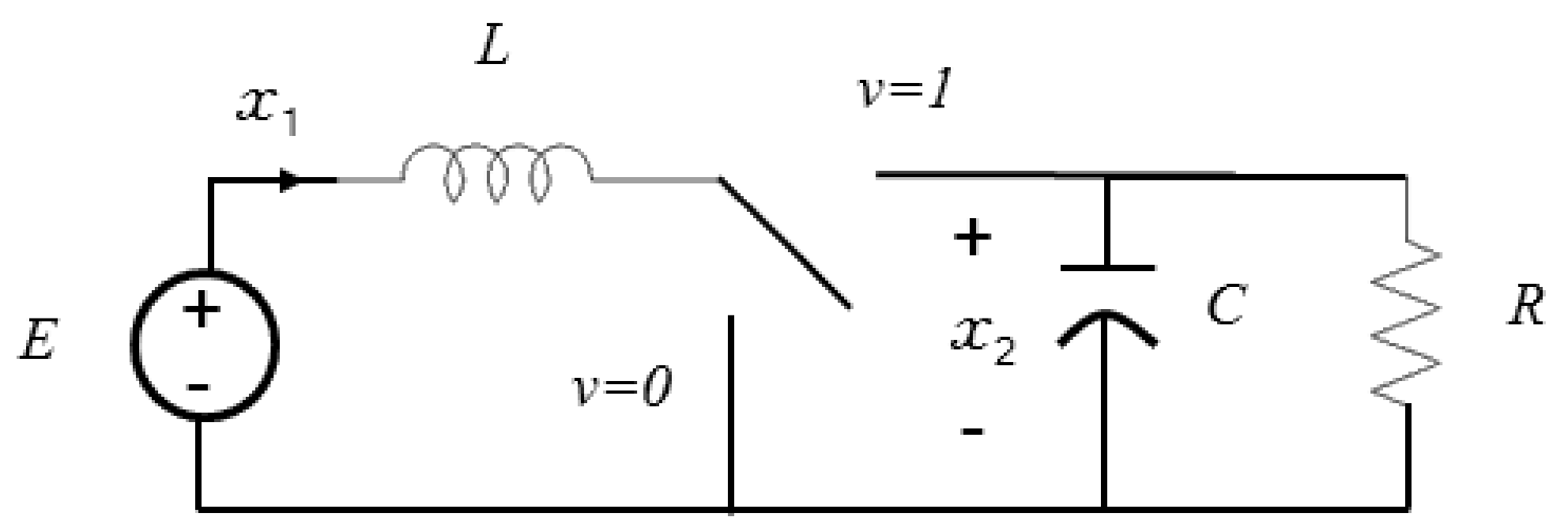
Figure 2.
Output tracking of the capacitor voltage. Reference signal in dashed line, and capacitor voltage in solid line. (a) Proposed controller. (b) Controller in [8]. (c) Controller in [40].
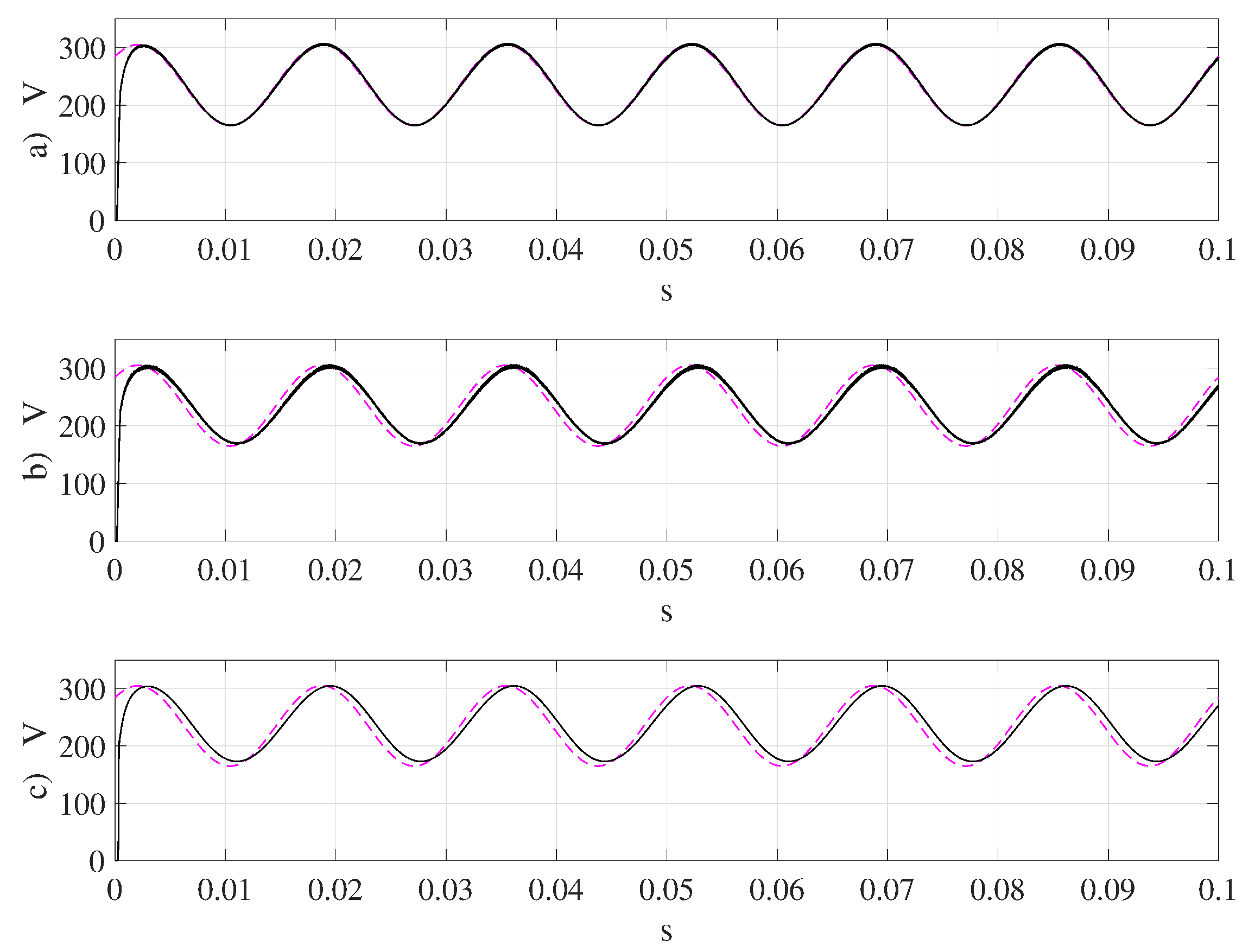
Figure 3.
Output tracking of the inductor current. Reference signal in dashed line, and inductor current in solid line. (a) Proposed controller. (b) Controller in [8]. (c) Controller in [40].
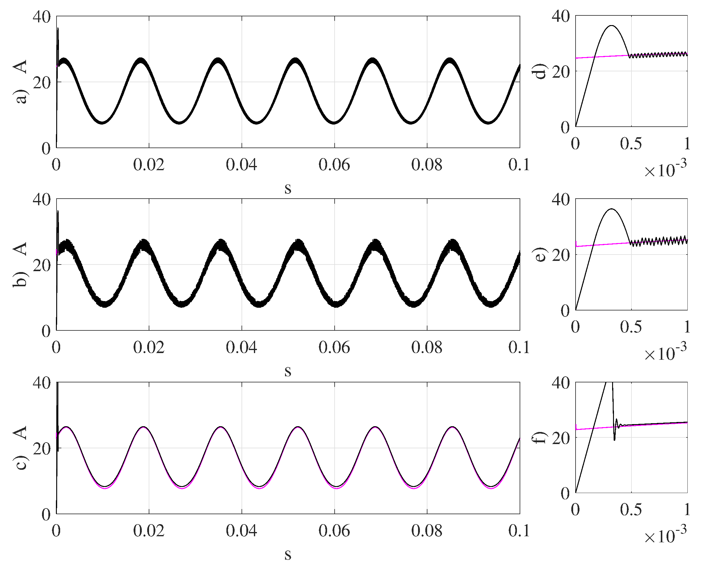
Figure 4.
Block diagram of the experimental setup.
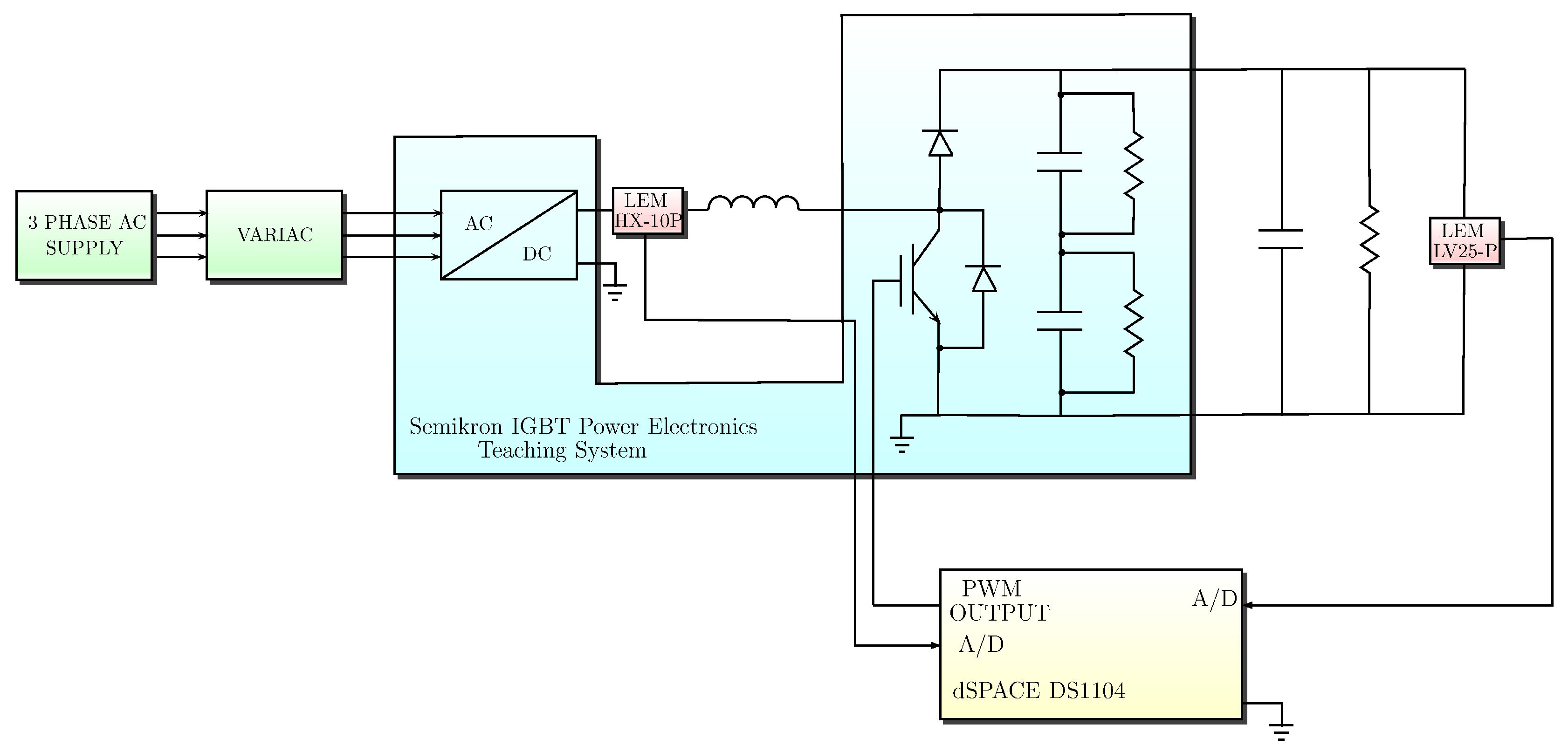
Figure 5.
Output tracking of the capacitor voltage with (60 Hz). Reference signal in dashed line, and capacitor voltage in solid line.
Figure 5.
Output tracking of the capacitor voltage with (60 Hz). Reference signal in dashed line, and capacitor voltage in solid line.
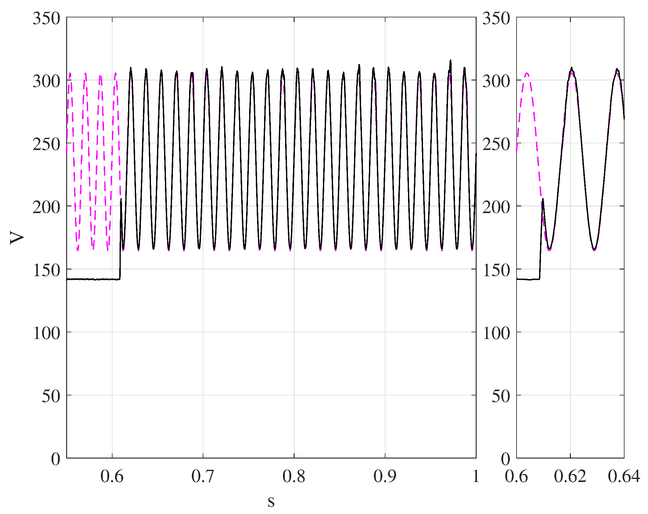
Figure 6.
Output tracking of the inductor current with (60 Hz). Reference signal in dashed line, and inductor current in solid line.
Figure 6.
Output tracking of the inductor current with (60 Hz). Reference signal in dashed line, and inductor current in solid line.

Figure 7.
Output tracking of the capacitor voltage with (50 Hz). Reference signal in dashed line, and capacitor voltage in solid line.
Figure 7.
Output tracking of the capacitor voltage with (50 Hz). Reference signal in dashed line, and capacitor voltage in solid line.
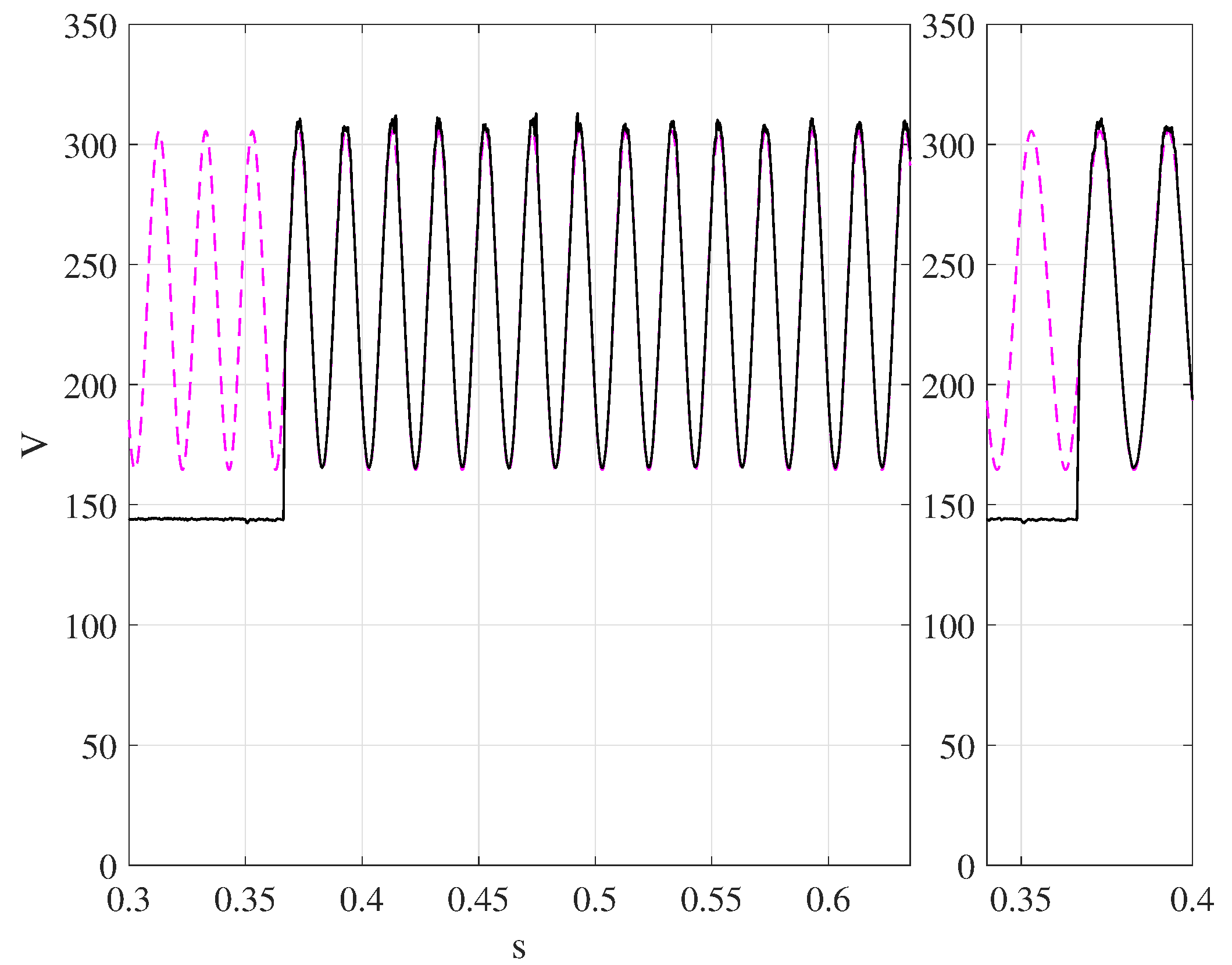
Figure 8.
Output tracking of the inductor current with (50 Hz). Reference signal in dashed line, and inductor current in solid line.
Figure 8.
Output tracking of the inductor current with (50 Hz). Reference signal in dashed line, and inductor current in solid line.
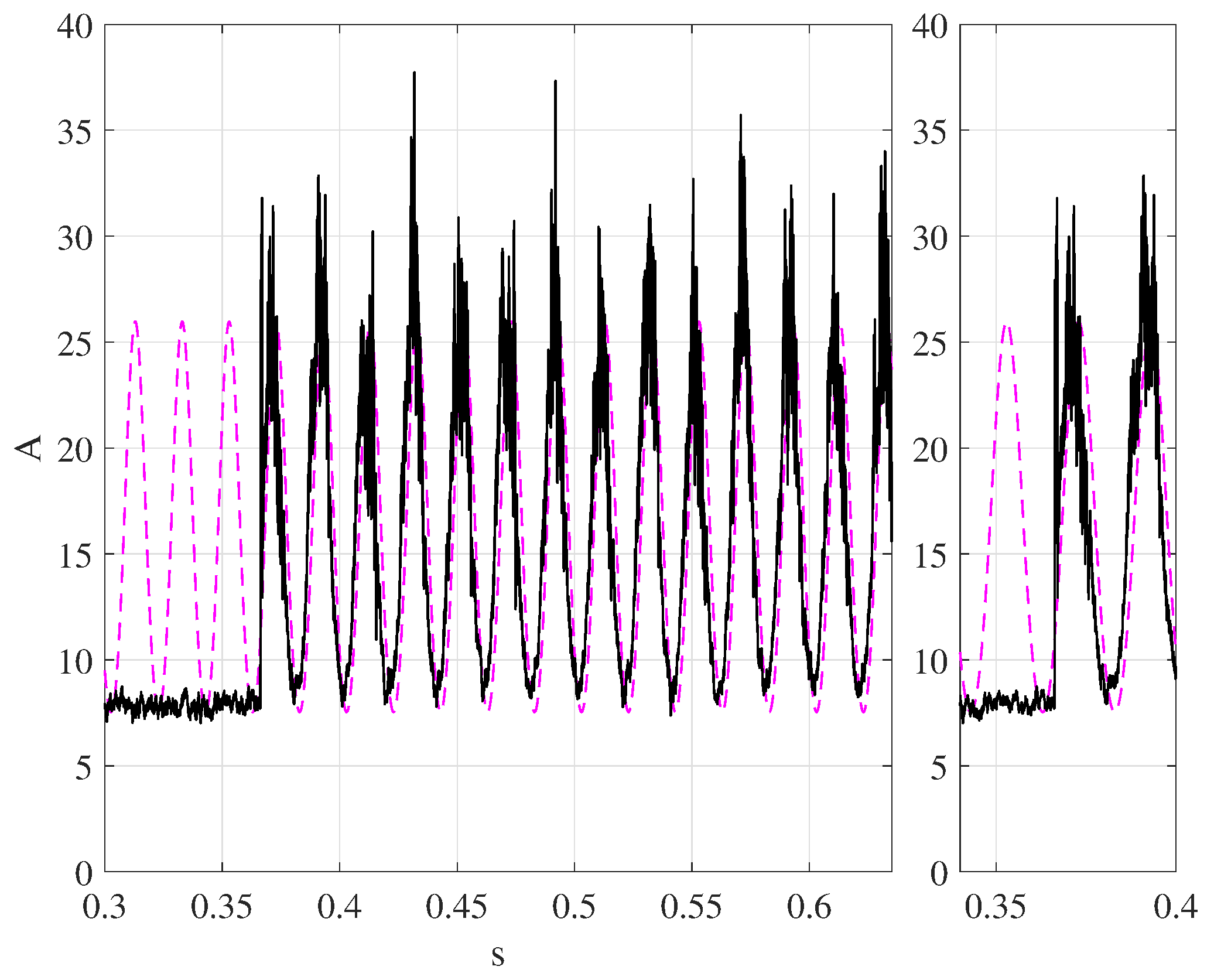
Figure 9.
Output voltage harmonic content with (60 Hz).
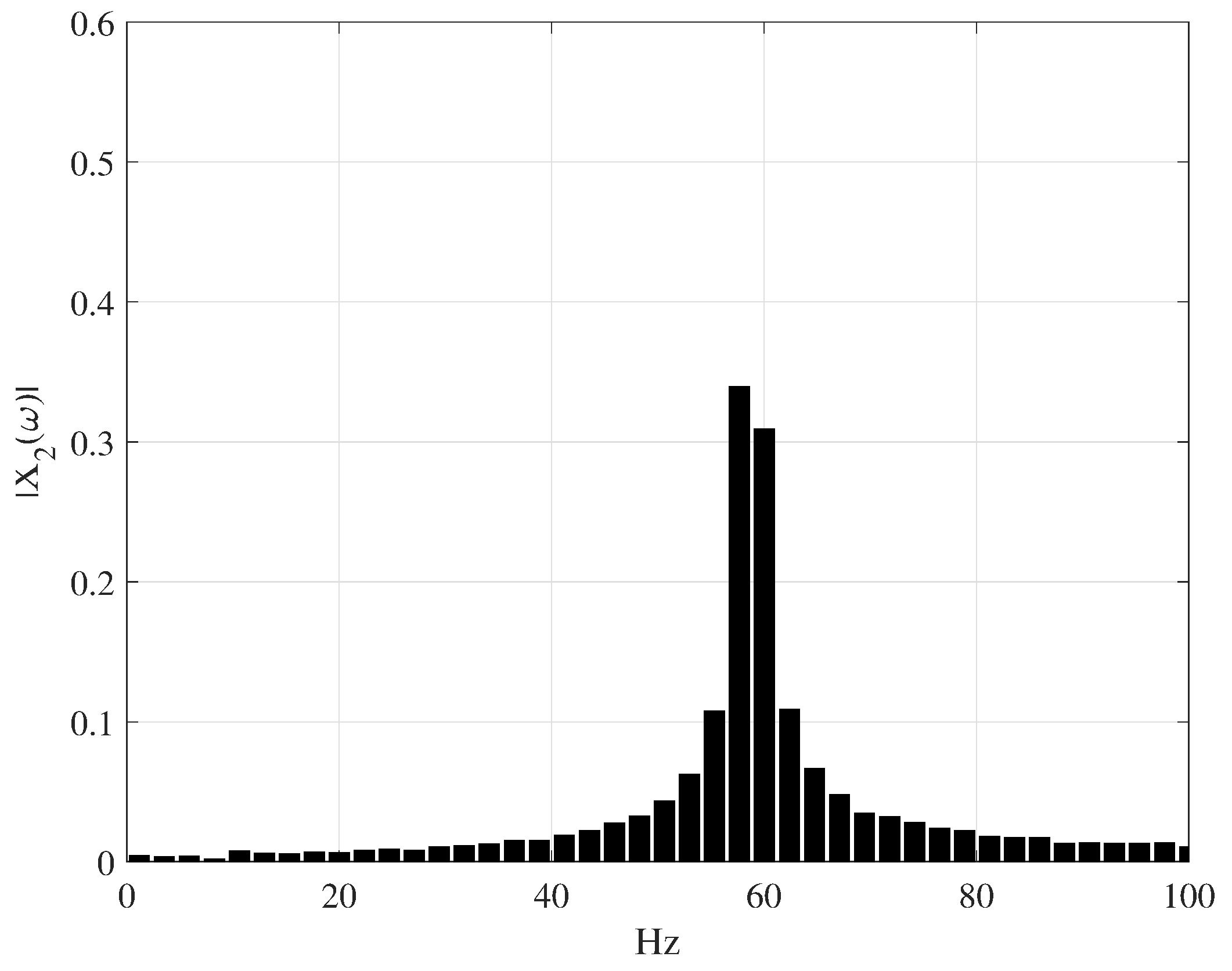
Figure 10.
Output voltage harmonic content with (50 Hz).

© 2019 by the authors. Licensee MDPI, Basel, Switzerland. This article is an open access article distributed under the terms and conditions of the Creative Commons Attribution (CC BY) license (http://creativecommons.org/licenses/by/4.0/).
Share and Cite
MDPI and ACS Style
Rivera, J.; Ortega-Cisneros, S.; Chavira, F. Sliding Mode Output Regulation for a Boost Power Converter. Energies 2019, 12, 879. https://doi.org/10.3390/en12050879
AMA Style
Rivera J, Ortega-Cisneros S, Chavira F. Sliding Mode Output Regulation for a Boost Power Converter. Energies. 2019; 12(5):879. https://doi.org/10.3390/en12050879
Chicago/Turabian StyleRivera, Jorge, Susana Ortega-Cisneros, and Florentino Chavira. 2019. "Sliding Mode Output Regulation for a Boost Power Converter" Energies 12, no. 5: 879. https://doi.org/10.3390/en12050879
Note that from the first issue of 2016, this journal uses article numbers instead of page numbers. See further details here.