Investigation of the Effect of Natural Fractures on Multiple Shale-Gas Well Performance Using Non-Intrusive EDFM Technology


1
State Key Laboratory of Shale Oil and Gas Enrichment Mechanisms and Effective Development, Beijing 100083, China
2
Hildebrand Department of Petroleum and Geosystems Engineering, The University of Texas at Austin, Austin, TX 78712, USA
3
Key Laboratory of Shale Oil/Gas Exploration & Production, SINOPEC, Beijing 100083, China
4
Institute of Nuclear and New Energy Technology, Tsinghua University, Beijing 100084, China
*
Authors to whom correspondence should be addressed.
Energies 2019, 12(5), 932; https://doi.org/10.3390/en12050932
Submission received: 4 January 2019
/
Revised: 26 February 2019
/
Accepted: 6 March 2019
/
Published: 10 March 2019
(This article belongs to the Special Issue Improved Reservoir Models and Production Forecasting Techniques for Multi-Stage Fractured Hydrocarbon Wells)
Abstract
:The influence of complex natural fractures on multiple shale-gas well performance with varying well spacing is poorly understood. It is difficult to apply the traditional local grid refinement with structured or unstructured gridding techniques to accurately and efficiently handle complex natural fractures. In this study, we introduced a powerful non-intrusive embedded discrete fracture model (EDFM) technology to overcome the limitations of exiting methods. Through this unique technology, complex fracture configurations can be easily and explicitly embedded into structured matrix blocks. We set up a field-scale two-phase reservoir model to history match field production data and predict long-term recovery from Marcellus. The effective fracture properties were determined thorough history matching. In addition, we extended the single-well model to include two horizontal wells with and without including natural fractures. The effects of different numbers of natural fractures on two-well performance with varying well spacing of 200 m, 300 m, and 400 m were examined. The simulation results illustrate that gas productivity almost linearly increases with the number of two-set natural fractures. Furthermore, the difference of well performance between different well spacing increases with an increase in natural fracture density. A larger well spacing is preferred for economically developing the shale-gas reservoirs with a larger natural fracture density. The findings of this study provide key insights into understanding the effect of natural fractures on well performance and well spacing optimization.
1. Introduction
Typical shale gas reservoirs consist of free gas and adsorbed gas. Economic shale gas production has been enabled by the advanced technologies of multiple horizontal wells and multi-stage hydraulic fracturing. The U.S. Energy Information Administration (EIA) estimates that dry shale gas production (0.48 trillion cubic meters) accounts for around 62% of the total U.S. dry natural gas production in 2017 [1]. The Marcellus shale formation is the most productive gas field in the United States. It has been reported that natural fractures are commonly observed in many shale gas formations based on outcrops, cores and image logs [2]. Engelder et al. [3] observed that there are two sets of natural fractures or two regional joint sets (J1 and J2 sets) in the Marcellus shale formation, which significantly affect the successful hydraulic fracturing treatment. A better understanding of natural fracture effects on well performance plays an important role in well spacing optimization of shale gas reservoirs.
The reactivation of pre-existing natural fractures during the hydraulic fracturing process is an important factor to create complex fracture networks, which have been observed and predicted by many examples of microseismic event patterns [4,5] and complex fracture propagation models [6,7,8,9,10,11]. Complex fracture networks will create a large productive fracture surface area, which is necessary to maximize shale-gas production. Based on the history matching results with an actual shale-gas well, Yu et al. [12] compared the long-term well productivity between simple and complex fracture geometries and found that complex fracture networks can produce 36.4% more gas recovery after 30 years than the simple fractures. Yu et al. [13] built a synthetic single shale-gas well model including 11 planar hydraulic fractures and 200 natural fractures. The authors found that the well performance of 200 two-set natural fractures is much better than that of 200 one-set natural fractures due to the formation of a much more complex connected fracture network. An increase of gas recovery of about 23.2% was achieved by the 200 two-set natural fractures when compared to the base model without natural fractures. Although there are many existing reservoir simulation studies for well spacing optimization in shale gas reservoirs [14,15,16,17,18,19], the influence of natural fractures on multiple shale-gas well performance with varying well spacing has not been well examined and understood.
Although there are many analytical or semi-analytical models to simulate shale-gas reservoirs [20,21,22,23], numerical reservoir simulation is needed to accurately model multiple shale-gas well production due to complexity of natural and hydraulic fracture configurations and complex two-phase flow physics [24,25,26,27]. The traditional local grid refinement (LGR) method with structured grids is difficult to model complex fractures explicitly [28,29]. Although the LGR method with unstructured grids has the capability to handle complex fractures, the computational efficiency is a big issue. In addition, advanced parallel computing power is generally needed. Furthermore, when performing sensitivity studies and history matching with varying fracture geometries such as fracture number, length, and height, re-gridding of matrix blocks containing fractures is required. In our previous work, we developed an innovative non-intrusive embedded discrete fracture model (EDFM) technology in conjunction with any third-party reservoir simulators with structured grids to accurately and efficiently handle any complex hydraulic and natural fractures [30,31], which provides a unique solution to overcome the above limitations of existing methods. The non-intrusive feature means that we do not need to get access to the source code of commercial reservoir simulators and just modifying their input files.
In this study, we introduced the non-intrusive EDFM technology in conjunction with a commercial reservoir simulator of CMG-GEM [32] to simulate shale gas production considering complex natural fractures and two-phase flow (gas and water). Based on an actual shale-gas well with available gas and water flow rates from the Marcellus shale formation, we build a field-scale reservoir model to perform history matching with gas and water flow rates under the flowing bottomhole pressure (BHP) constraint. After history matching, we predict a 30-year production forecasting. Subsequently, we extend the history-matched reservoir model with effective fracture properties to include two horizontal wells with three different well spacing values of 200, 300 and 400 m. In addition, the impacts of different numbers of natural fractures such as 100, 1000, 5000, and 100,000 on multiple shale-gas well performance are investigated. The effect of natural fracture density on well spacing optimization and pressure distribution is discussed.
2. Methodology
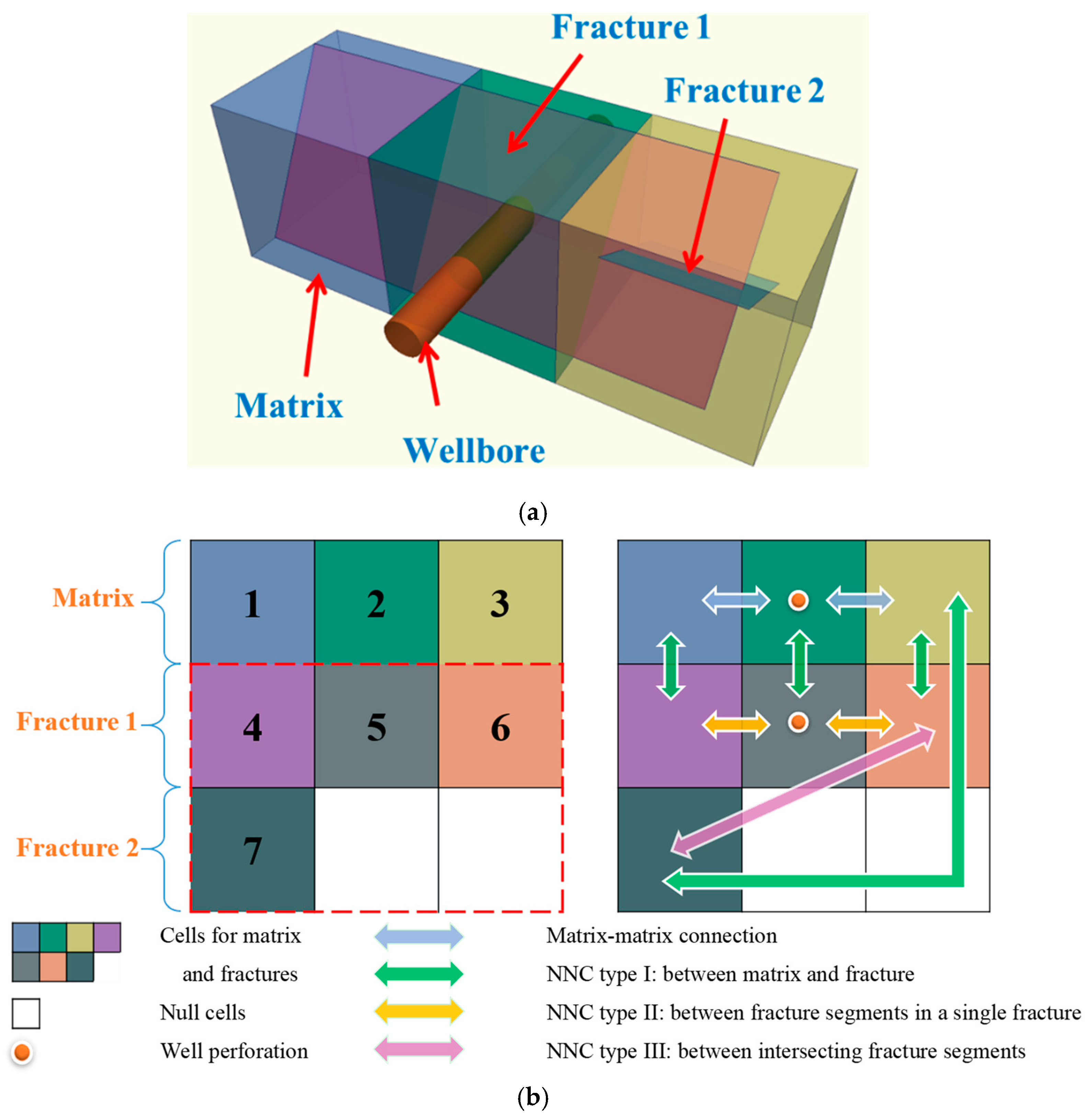
The non-intrusive EDFM technology in conjunction with the commercial reservoir simulator was originally developed by Xu et al. [30,31]. Here, we only briefly introduced this powerful technology. Based on the non-intrusive EDFM technology, both 3D complex hydraulic and natural fractures in the physical domain can be directly and explicitly embedded into the simple structured matrix grids, as demonstrated in Figure 1a. Based on the intersections between complex fractures and matrix grids, a number of extra fracture grids will be generated, as shown in Figure 1b [30]. In Figure 1, two 3D fractures are explicitly embedded into three matrix grids in the physical domain. Correspondingly, an additional four fracture grids are created in the computational domain. Multi-phase flow such as gas and water between matrix and fracture grids can be conveniently simulated through calculating transmissibility between these non-neighboring connections (NNCs) grids, as shown in different colors of arrows of Figure 1b, which is a general feature for commercial reservoir simulators to handle faults before. A non-intrusive EDFM preprocessor has been developed to automatically check the complex intersections of fractures and matrix grids and calculate the transmissibility and other physical properties of the additional fracture grids such as porosity and depth, which are needed to input for the commercial reservoir simulator.
There are three types of NNCs including NNC type I, which is the connection between matrix and fracture, NNC type II, which is the connection between fracture segments in a single fracture, and NNC type III, which is the connection between intersecting fracture segments [30]. The flow rate (, m3/s) of phase l between NNC grids is calculated by the following equation:
where λl represents the relative mobility of phase l (cp−1), Δpl represents the pressure difference between NNC grids (Pa), TNNC represents the transmissibility factor of NNC grids (mD-m), which can be calculated by:
where kNNC represents the matrix grid permeability for NNC type I and average fracture permeability for NNC types II and III (mD); ANNC represents the contact area between NNC grids (m2); dNNC represents the connection distance between different NNC grids (m). It should be mentioned that the non-intrusive EDFM technology only deals with the transmissibility factor and does not involve relative phase mobility calculation. Hence, it can be applied in both black oil simulation and compositional simulation.
For the connection between fractures and wellbore, the following effective wellbore index (, mD-m) will be calculated [30]:
where kf is the fracture permeability (mD), wf is fracture width (m), L is fracture segment length (m), W is fracture segment height (m), and rw is the wellbore radius (m).
The validation of this methodology against the traditional LGR method can be found in our previous work [30,31]. The efficiency of the EDFM method is much higher than the LGR method, especially when dealing with multiple wells with a large number of fractures [33]. It has been widely applied to model well interference due to complex fracture hits [34,35], automatic history matching for shale reservoirs [36,37,38], gas injection for enhanced unconventional oil recovery [39,40,41], and naturally fractured reservoir simulation [42].
3. Field Case Study of Single Shale-Gas Well
3.1. History Matching
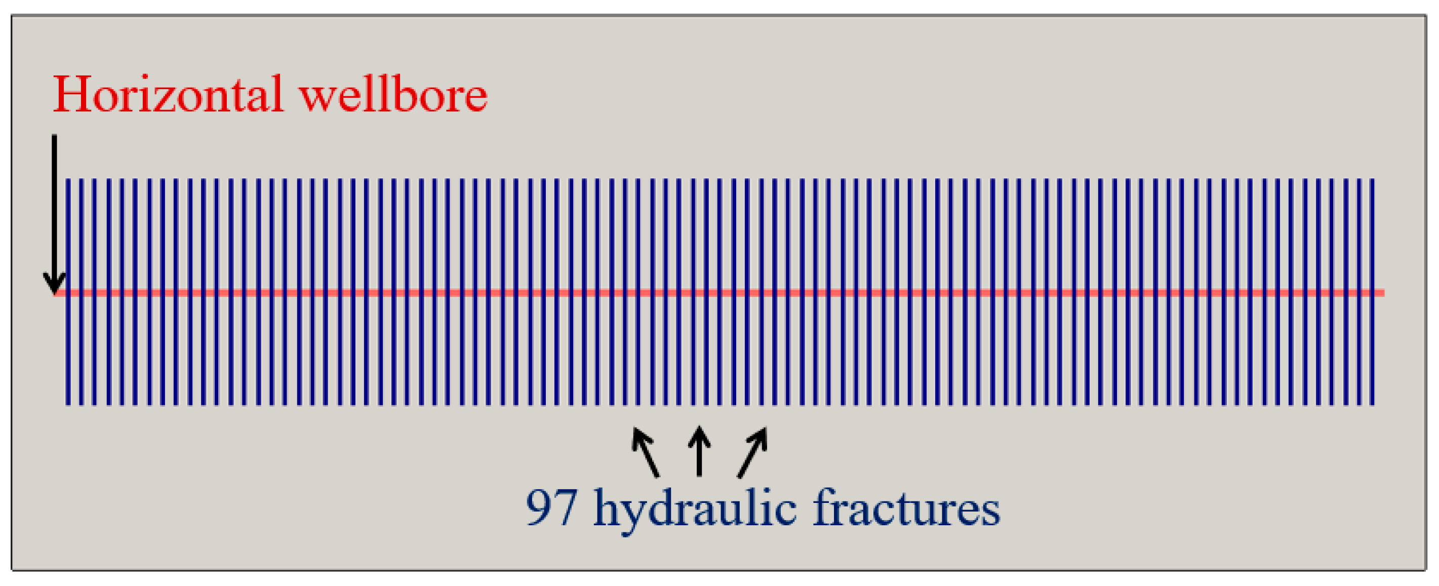
An actual Marcellus shale-gas well with available 486-day gas and water production data was selected to perform history matching. The well has 11 perforations stages with a cluster spacing of 15.24 m and was hydraulically fractured using 16,770 m3 water and 2,895,956 kg proppant. The lateral length of horizontal wellbore is about 1382 m. There are 10 stages with nine clusters per stage and one stage with seven clusters, so 97 effective hydraulic fractures were assumed in the following simulation study.
We set up a field-scale shale-gas reservoir model with two-phase flow (gas and water) using a compositional numerical reservoir simulator [32], as shown in Figure 2. The gas type is methane. The dimension of the reservoir model without embedding hydraulic fractures is 1585 m × 622 m × 27.6 m and it is assumed that the reservoir thickness was fully penetrated by hydraulic fractures. Hence, the effective hydraulic fracture height is 27.6 m. The matrix grid size is 6 m × 12 m × 27.6 m in x, y, and z directions.
The number of matrix grids is 13,260. Hydraulic fractures were modeled using the non-intrusive EDFM method. After embedding 97 hydraulic fractures with fracture half-length of 127 m into matrix grids, an extra number of fracture grids of 2040 was generated along the x direction. The fracture grid size remains the same as the matrix grid size. The model dimension with hydraulic fractures becomes 1828.8 m × 622 m × 27.6 m. It is assumed that both matrix and fracture grids have the same gas-water relative permeability curve, which is from the work by Yu et al. [38]. In addition, the experimental measurements of gas desorption are considered in the simulation model [38]. The other reservoir and fracture parameters are listed in Table 1.
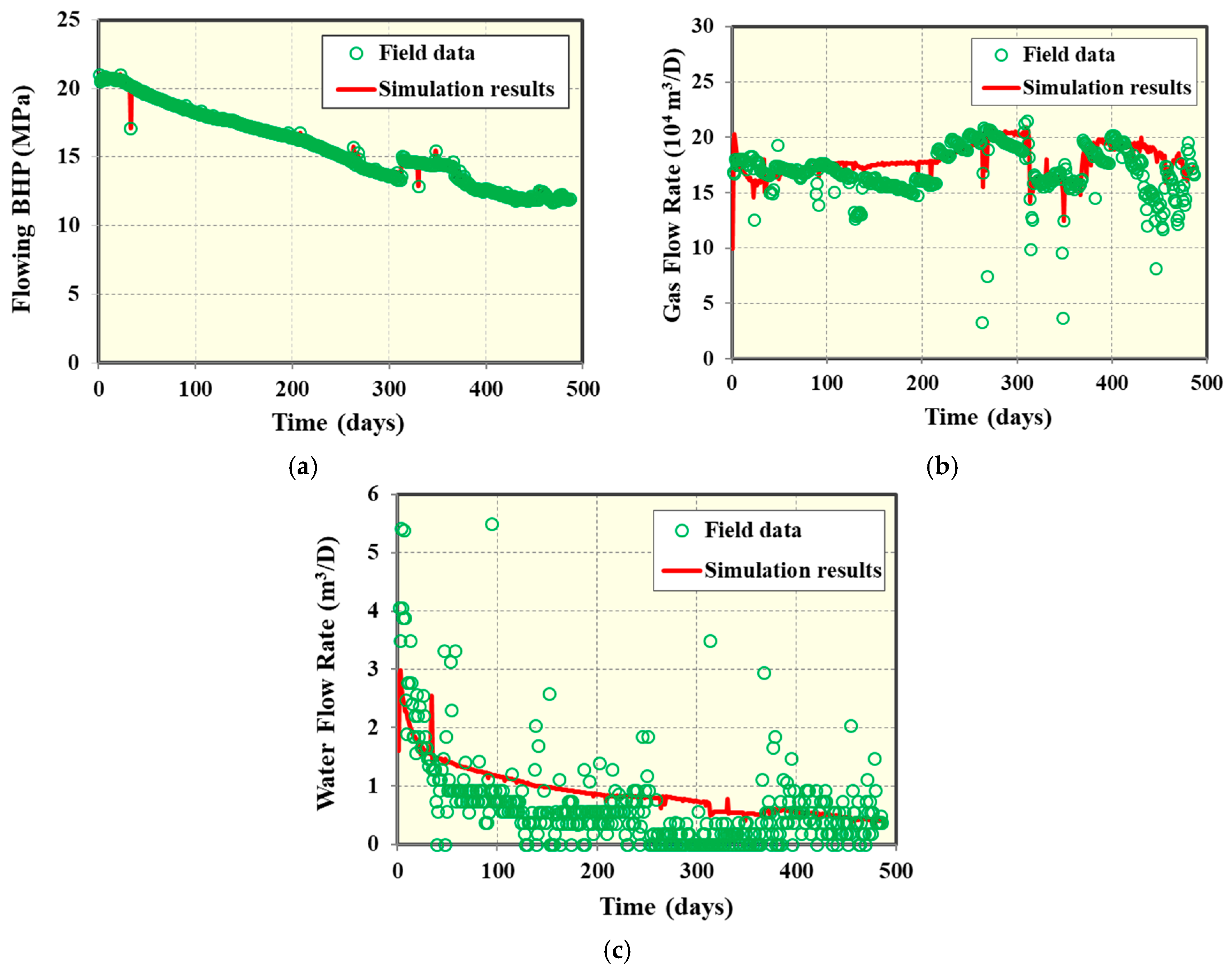
During the history-matching process, we applied the measured flowing BHP for the reservoir simulation constraint, as shown in Figure 3a. In order to achieve good match results with measured gas and water flow rates, we mainly tune matrix permeability, fracture half-length, fracture conductivity, and fracture water saturation because these parameters are very sensitive for tuning and performing history matching.
It should be mentioned that the fracture water saturation is higher than the matrix water saturation because water is more difficult to transport into the matrix than into the fracture due to lower matrix permeability. Figure 3b,c present the comparison of gas and water flow rates between filed data and simulation results. The relative error of history-matching results for gas flow rate is about 10%. It can be illustrated that reasonable agreements were obtained. The final history-matching tuning parameters were determined as matrix permeability of 0.000525 mD, fracture half-length of 127 m, fracture conductivity of 0.73 mD-m, and fracture water saturation of 37.4%. It should be noted that fracture half-length has an important impact on multiple shale-gas well placement. In general, longer fracture half-length will result in larger well spacing.
3.2. Production Forecasting
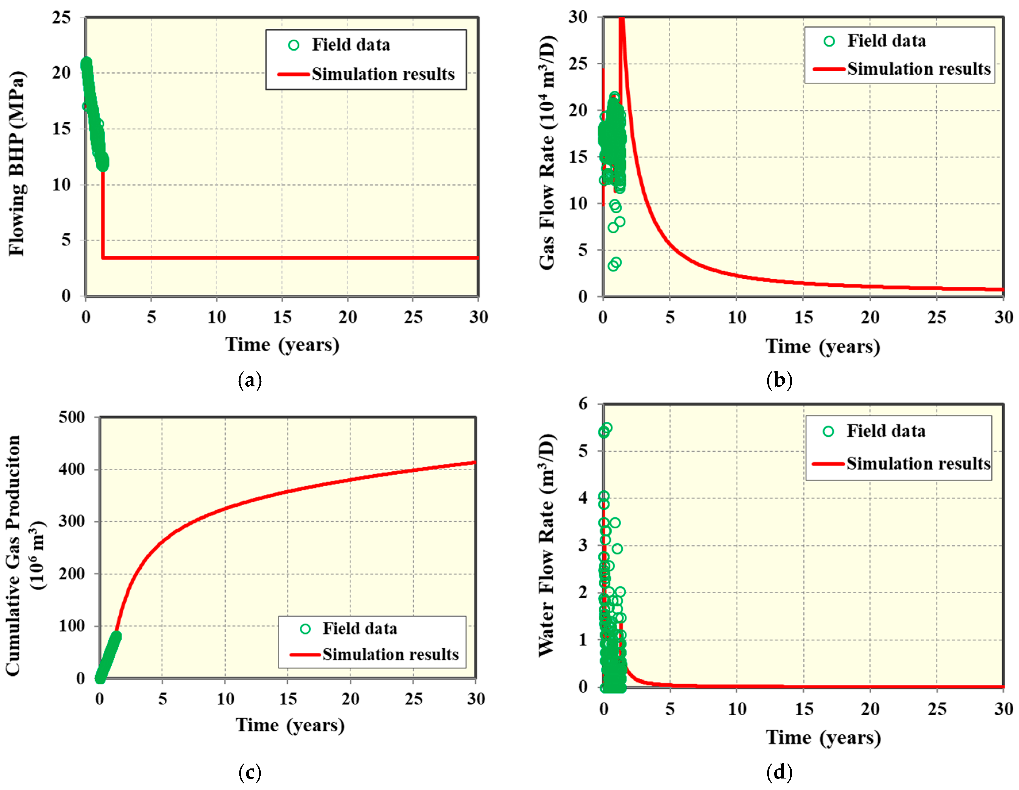
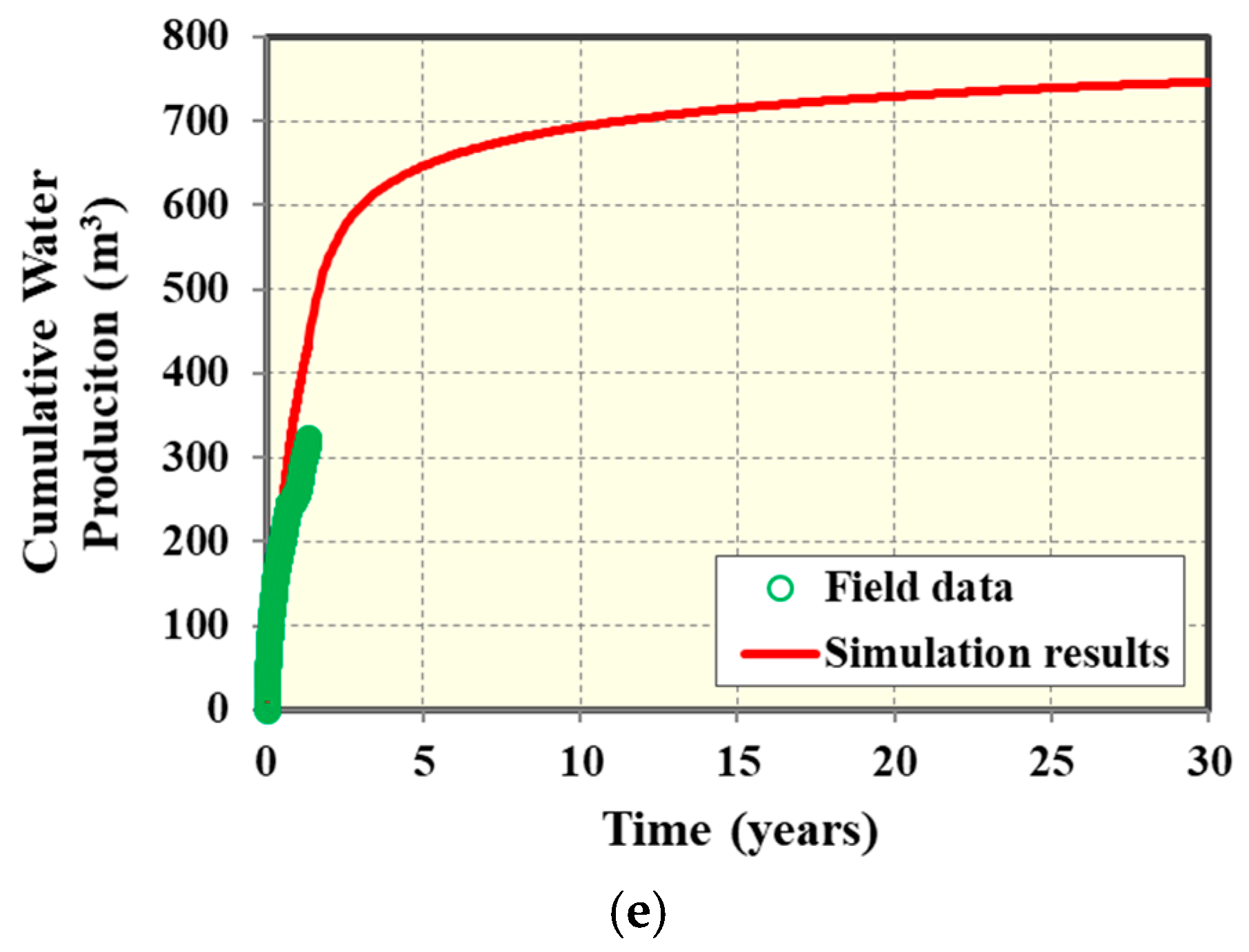
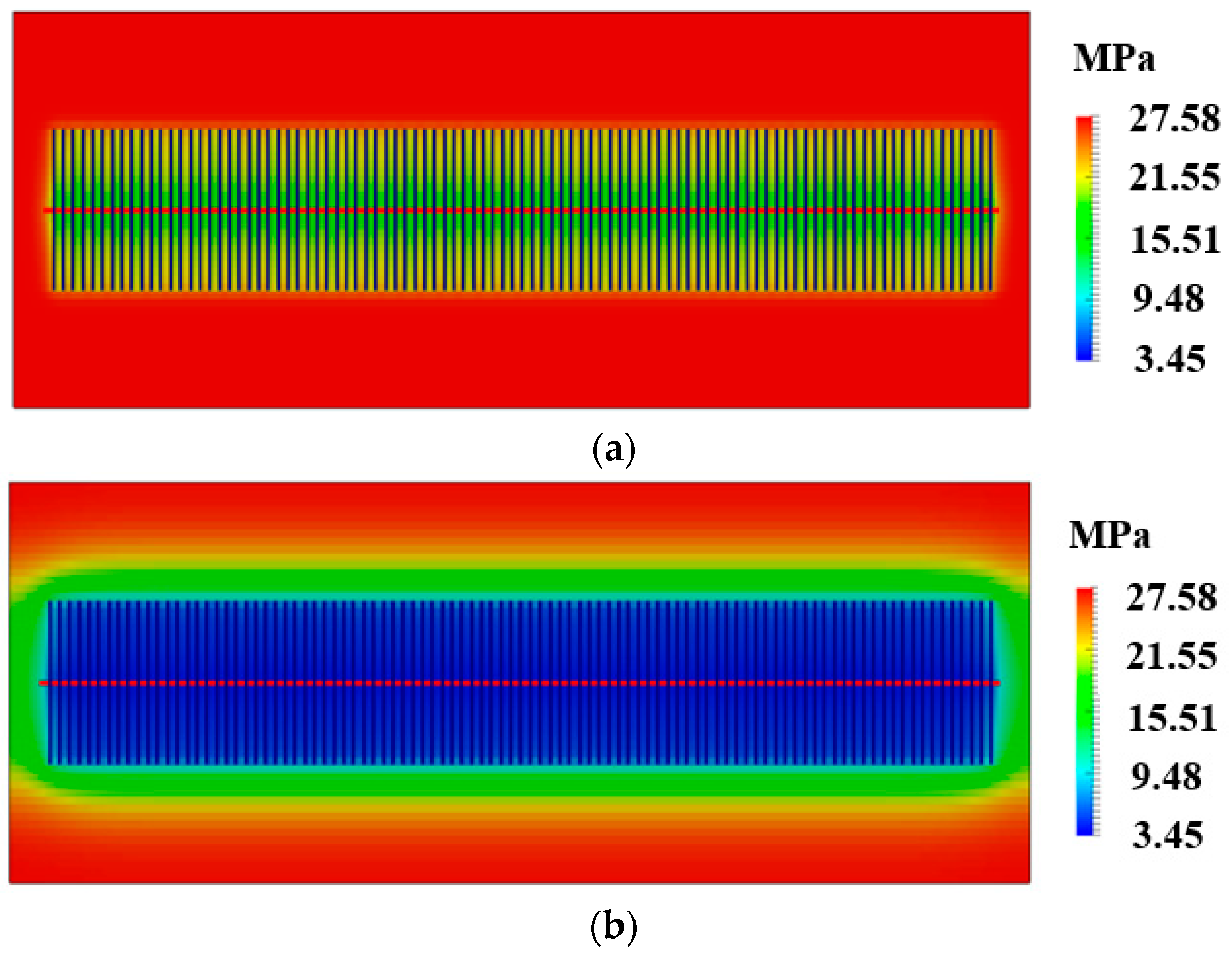
After the history-matching process, we performed long-term production forecasting for 30 years. Since there are no available actual well control information for prediction, a constant flowing BHP of 3.45 MPa after the history-matching period was assumed for the simulation constraint, as illustrated in Figure 4a. Figure 4b,c show the prediction of gas flow rate and cumulative gas production incorporating a short-term field data, respectively. As shown, the estimated ultimate recovery (EUR) after 30 years for this shale-gas well is about 413 × 106 m3. Figure 4d,e show the prediction of water flow rate and cumulative water production incorporating the short-term field data, respectively. It can be seen that the water flow rate becomes negligible after around three years. The cumulative water production after 30 years for this shale-gas well is about 747 m3. Figure 5 compares the pressure distribution after the history-matching period and 30 years of production, clearly illustrating different drainage area and production interference intensity between hydraulic fractures. It can be observed that a stronger production interference between hydraulic fractures occures after 30 years of production when compared to that after the history-matching period. In addition, a larger effective drainage area can be generated after 30 years of production.
4. Basic Reservoir Model of Two Shale-Gas Wells
4.1. Varying Well Spacing without Natural Fractures
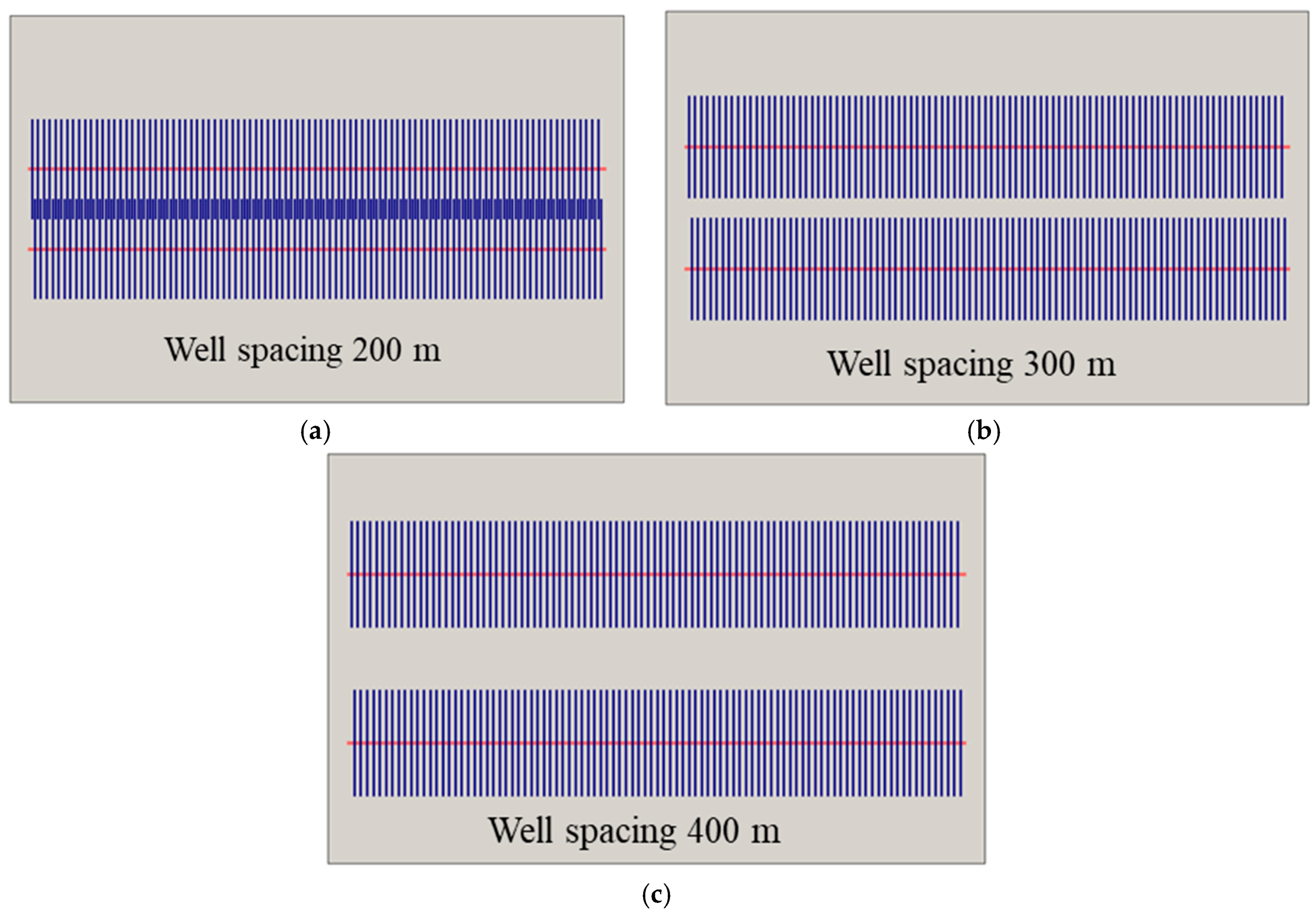
Based on the history-matching results from the field-scale shale-gas model, we extended the reservoir model to include two horizontal shale-gas wells with varying well spacing and each well has 97 hydraulic fractures. The effect of natural fractures was not considered in this basic model. The model dimension without embedding hydraulic fractures is 1585 m × 975 m × 27.6 m and fractures fully penetrate the reservoir thickness. The matrix grid size is 6 m × 12 m × 27.6 m in x, y, and z directions. The number of matrix grids is 20,800. Three different well spacing values such as 200 m, 300 m, and 400 m were investigated, as depicted in Figure 6. The placement of hydraulic fractures from two horizontal wells has a staggered pattern. As shown in Figure 6a, there is about 21% overlap of fracture half-length. The distance between neighboring fracture tips of two wells is 47.5 m and 148 m for well spacing of 300 m and 400 m, respectively, as shown in Figure 6b,c. After embedding 194 hydraulic fractures into matrix grids, an extra number of fracture grids of 4320 were generated along the x direction. The grid size of fracture grids is the same as the matrix grid size. The final model dimension becomes 1914 m × 975 m × 27.6 m. All fracture and reservoir properties remain the same as those of field case study with good history matching results. A constant flowing BHP of 3.45 MPa was applied in the 30-year simulation constraint.
4.2. Varying Well Spacing with Natural Fractures
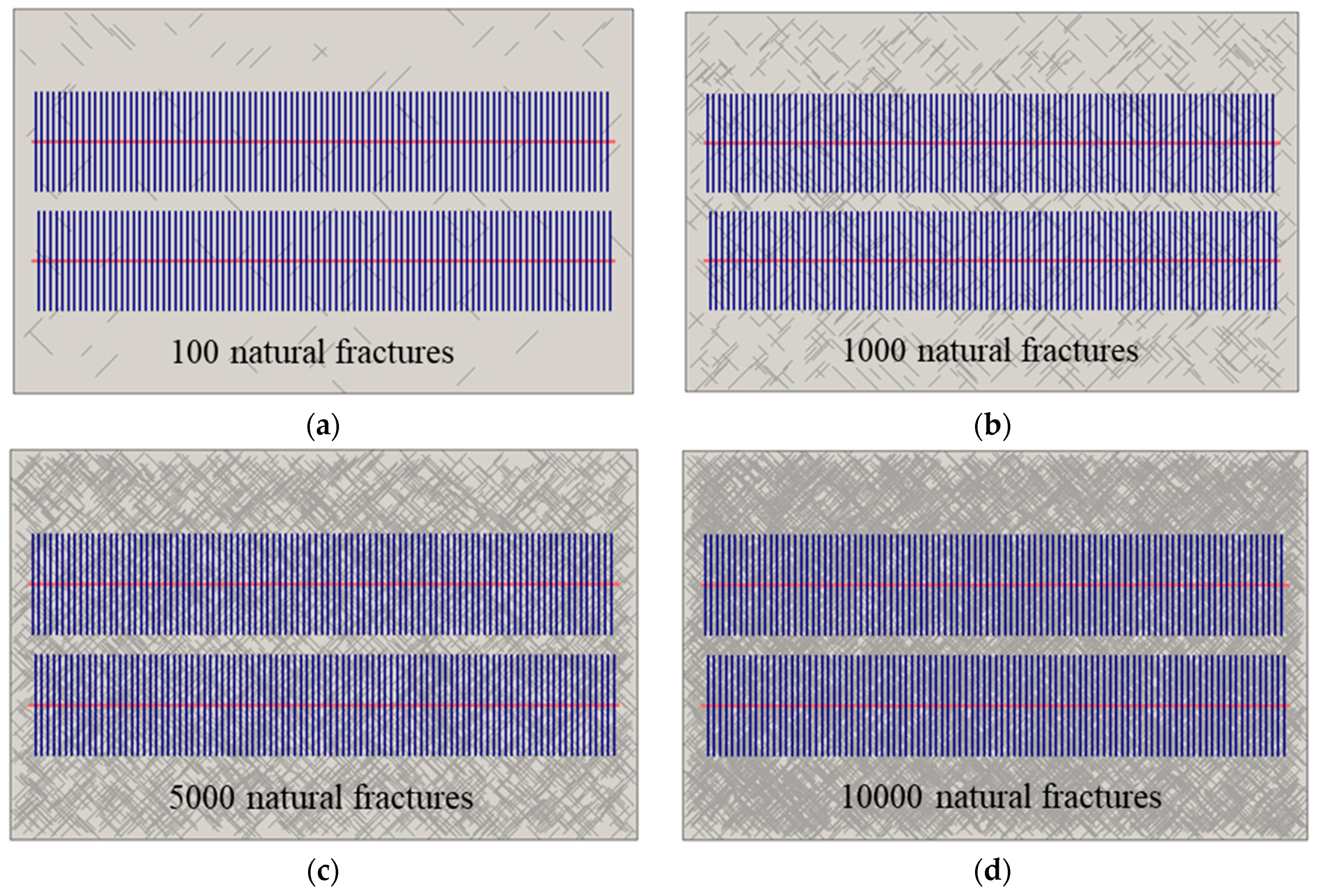
Next, the effect of natural fractures with different numbers was considered in the basic reservoir model with varying well spacing. Four different numbers of natural fractures such as 100, 1000, 5000, and 10,000 were investigated in this study. It should be mentioned that hydraulic fractures are non-planar if considering the interaction between pre-existing natural fracture with hydraulic fracture using fracture propagation models [6,7,8]. However, hydraulic fractures are assumed to be planar in this study. We did not apply the fracture propagation model to predict complex fracture network. Figure 7 displays the natural fracture distribution of four different cases using an example of the well spacing of 300 m. We applied a statistical method to generate the locations of natural fractures, which are normally distributed in the reservoir model. For each case, there are two sets of natural fractures and each set has the same number of natural fractures. One set of natural fractures has an orientation of 45 degrees with respect to the x axis. Another set has an orientation of 135 degrees along the x axis. The natural fractures have a range of length from 30 m to 91 m. The natural fracture conductivity for each case is assumed to be 0.03 mD-m with natural fracture aperture of 0.003 m. The natural fractures fully penetrate the reservoir thickness. It should be mentioned that the impacts of natural fracture conductivity, length, and orientation are not examined in this study. After embedding natural and hydraulic fractures together into matrix grids with well spacing of 300 m, an extra number of fracture grids of 5520, 15,840, 62,000, and 119,440 were generated for the number of natural fractures of 100, 1000, 5000, 10,000, respectively, along the x direction. As can be seen that, the extra number of fractures grids is larger than the number of matrix grids of 20,800 for the 5000 and 10,000 natural fractures. With the increasing number of natural fractures, there are more interactions between natural and hydraulic fractures, resulting in more well interference due to complex fracture connections.
5. Results and Discussion
5.1. Effect of Natural Fractures on Well Performance
The effects of different numbers of natural fractures on cumulative gas production are compared in Figure 8, Figure 9 and Figure 10 for well spacings of 200, 300 and 400 m, respectively. It can be clearly observed that a larger number of natural fractures contributes to more production. The incremental EUR after 30 years compared to the case with well spacing of 200 m without natural fractures is about 1.5%, 13.8%, 69%, and 130.7% for the fracture number of 100, 1000, 5000, and 10,000, respectively. When compared to the case with well spacing of 300 m, the incremental EUR after 30 years of production is about 1.4%, 13.9%, 66.7%, and 124.3% for the fracture number of 100, 1000, 5000, and 10,000, respectively. When compared to the case with well spacing of 400 m, the incremental EUR after 30 years of production is about 1.6%, 15.3%, 72.6%, and 131% for the fracture number of 100, 1000, 5000, and 10,000, respectively. For 100 natural fractures, there is only a smaller number of natural fractures connecting with hydraulic fractures, leading to a slight increase of cumulative gas production. However, for 10,000 natural fractures, there is a much more complex connected fracture network between natural and hydraulic fractures, resulting in a big increase of contact area between fracture and matrix and a large increase of cumulative gas production. The CPU time for the model with well spacing of 300 m is about 5, 7 min 17 and 30 min, corresponding to the number of natural fractures of 100, 1000, 5000, and 10,000, respectively. Hence, the natural fractures play an important role in long-term multiple shale-gas well performance, which can be easily and efficiently handled by the non-intrusive EDFM technology.
5.2. Effect of Natural Fractures on Well Spacing Optimization
The effect of natural fracture density on the incremental gas production after 30 years under different well spacing is presented in Figure 11. Here, the natural fracture density refers to the number of natural fractures per 929 m2, which is about 0.06, 0.6, 3, and 6 for the total number of natural fractures of 100, 1000, 5000, and 10,000, respectively. The incremental gas production after 30 years means that the difference of cumulative gas production with and without natural fractures under a given well spacing. It can be clearly seen that the incremental gas production of different well spacing with and without natural fractures almost linearly increases with the increasing natural fracture density. In addition, the difference of incremental gas production between different well spacing increases with an increase in natural fracture density. The difference of incremental gas production between well spacing of 200 m and 400 m under the natural fracture density of 0.06, 0.6, 3 and 6 per 929 m2 is about 3.2 × 10⁶ m3, 31.2 × 10⁶ m3, 125.6 × 10⁶ m3, and 184.7 × 10⁶ m3, respectively. Consequently, it can be implied that a larger well spacing is preferred for the shale-gas reservoir with a larger natural fracture density.
5.3. Effect of Natural Fractures on Pressure Distribution
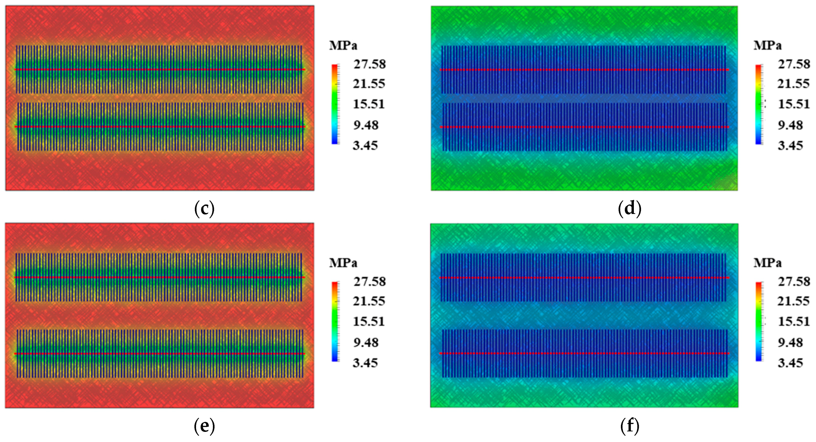
Figure 12 and Figure 13 compare pressure distribution after one and 30 years of production under different well spacing with and without natural fractures. The extreme case with 10,000 natural fractures was plotted for comparison. As shown, different drainage area at early and later time of production can be clearly observed. In addition, a stronger well interference between two wells after 30 years under a smaller well spacing occurs. Especially, the drainage area expands more when considering a bigger number of natural fractures.
6. Conclusions
We applied the non-intrusive EDFM technology as well as a compositional reservoir simulator to perform shale-gas two-phase flow simulations. The impact of natural fractures on multiple shale-gas well performance with varying well spacing was investigated based on history matching results of an actual shale-gas well from Marcellus shale formation. The following conclusions can be drawn from this study:
- (1)
- The effective matrix and fracture properties were obtained based on good history matching results such as matrix permeability of 0.000525 mD, fracture half-length of 127 m, fracture conductivity of 0.73 mD-m, and fracture water saturation of 37.4%.
- (2)
- The EUR and cumulative water production after 30 years of the actual shale-gas well were determined as 413 × 106 m3 and 747 m3, respectively.
- (3)
- The effect of natural fractures on two shale-gas well performance almost linearly increases with the increasing number of natural fractures. For example, the natural fractures contribute to the incremental EUR after 30 years of 1.4%, 13.9%, 66.7%, and 124.3% for the well spacing of 300 m with fracture number of 100, 1000, 5000, and 10,000, respectively.
- (4)
- The CPU time for the model with well spacing of 300 m is about 30 min when dealing with 10,000 natural fractures based on the non-intrusive EDFM technology.
- (5)
- A larger number of natural fractures is easier to form a more complex connected fracture network with hydraulic fractures, resulting in a higher well productivity.
- (6)
- The difference of well performance between different well spacing increases with the increasing natural fracture density. For example, the difference of well performance between well spacing of 200 m and 400 m is about 3.2 × 10⁶ m3, 31.2 × 10⁶ m3, 125.6 × 10⁶ m3, and 184.7 × 10⁶ m3 corresponding to the natural fracture density of 0.06, 0.6, 3 and 6 per 929 m2, respectively.
- (7)
- This study provides a better understanding of the impact of complex natural fractures on multiple shale-gas well performance with varying well spacing. A larger well spacing is suggested when the shale-gas reservoir has a larger natural fracture density.
Author Contributions
Conceptualization, W.Y. and M.L.; methodology and investigation W.Y. and M.L.; writing—original draft preparation, W.Y.; writing—review and editing, X.H.; project administration, W.W.; funding acquisition, W.Y., M.L. and W.W.
Funding
This research was funded by “National Science and Technology Major Project of China, grant number 2016ZX05061003-003”, “National Natural Science Foundation of China, grant number 51728401”.
Acknowledgments
We would like to acknowledge Computer Modelling Group Ltd. and SimTech LLC for providing the CMG-GEM and EDFM software for this investigation.
Conflicts of Interest
The authors declare no conflict of interest.
References
- U.S. Energy Information Administration. Available online: https://www.eia.gov/tools/faqs/faq.php?id=907&t=8 (accessed on 3 October 2018).
- Gale, J.F.W.; Laubach, S.E.; Olson, J.E.; Eichhubl, P.; Fall, A. Natural fractures in shale: A review and new observations. AAPG Bull. 2014, 98, 2165–2216. [Google Scholar] [CrossRef]
- Engelder, T.; Lash, G.G.; Uzcategui, R.S. Joint sets that enhance production from Middle and Upper Devonian gas shales of the Appalachian Basin. AAPG Bull. 2009, 93, 857–889. [Google Scholar] [CrossRef]
- Fisher, M.K.; Wright, C.A.; Davidson, B.M.; Steinsberger, N.P.; Buckler, W.S.; Goodwin, A.; Fielder, E.O. Integrating fracture mapping technologies to improve stimulations in the Barnett shale. SPE Prod. Facil. 2005, 20, 85–93. [Google Scholar] [CrossRef]
- Fisher, M.K.; Warpinski, N.R. Hydraulic-fracture-height growth: Real data. SPE Prod. Oper. 2012, 27, 8–19. [Google Scholar] [CrossRef]
- Wu, R.; Kresse, O.; Weng, X.; Cohen, C.; Gu, H. Modeling of interaction of hydraulic fractures in complex fracture networks. In Proceedings of the SPE Hydraulic Fracturing Technology Conference, The Woodlands, TX, USA, 6–8 February 2012. [Google Scholar]
- Wu, K.; Olson, J.E. Investigation of the impact of fracture spacing and fluid properties for interfering simultaneously or sequentially generated hydraulic fractures. SPE Prod. Oper. 2013, 28, 427–436. [Google Scholar] [CrossRef]
- Wu, K.; Olson, J.E. Simultaneous multifracture treatments: Fully coupled fluid flow and fracture mechanics for horizontal wells. SPE J. 2015, 20, 337–346. [Google Scholar] [CrossRef]
- Yue, K.; Olson, J.E.; Schultz, R.A. Layered modulus effect on fracture modeling and height containment. In Proceedings of the SPE/AAPG/SEG Unconventional Resources Technology Conference, Houston, TX, USA, 23–25 July 2018. [Google Scholar]
- Tang, J.; Wu, K.; Zeng, B.; Huang, H.; Hu, X.; Guo, X.; Zuo, L. Investigate effects of weak bedding interfaces on fracture geometry in unconventional reservoirs. J. Pet. Sci. Eng. 2018, 165, 992–1009. [Google Scholar] [CrossRef]
- Xie, J.; Huang, H.; Ma, H.; Zeng, B.; Tang, J.; Yu, W.; Wu, K. Numerical investigation of effect of natural fractures on hydraulic-fracture propagation in unconventional reservoirs. J. Nat. Gas Sci. Eng. 2018, 54, 143–153. [Google Scholar] [CrossRef]
- Yu, W.; Wu, K.; Liu, M.; Sepehrnoori, K.; Miao, J. Production forecasting for shale gas reservoirs with nanopores and complex fracture geometries using an innovative non-intrusive EDFM method. In Proceedings of the SPE Annual Technical Conference and Exhibition, Dallas, TX, USA, 24–26 September 2018. [Google Scholar]
- Yu, W.; Xu, Y.; Liu, M.; Wu, K.; Sepehrnoori, K. Simulation of shale gas transport and production with complex fractures using embedded discrete fracture model. AIChE J. 2018, 64, 2251–2264. [Google Scholar] [CrossRef]
- Díaz de Souza, O.C.; Sharp, A.J.; Martinez, R.C.; Foster, R.A.; Simpson, M.R.; Piekenbrock, E.J.; Abou-Sayed, I. Integrated unconventional shale gas reservoir modeling: A worked example from the Haynesville Shale, De Soto Parish, North Lousiana. In Proceedings of the SPE Americas Unconventional Resources Conference, Pittsburgh, PA, USA, 5–7 June 2012. [Google Scholar]
- Yu, W.; Sepehrnoori, K. Optimization of multiple hydraulically fractured horizontal wells in unconventional gas reservoirs. J. Pet. Eng. 2013, 2013. [Google Scholar] [CrossRef]
- Tung, Y.; Virues, C.; Cumming, J.; Gringarten, A. Multiwell deconvolution for shale gas. In Proceedings of the SPE Europec Featured at 78th EAGE Conference and Exhibition, Vienna, Austria, 30 May–2 June 2016. [Google Scholar]
- Manestar, G.J.; Thompson, A. Dual porosity modeling for shale gas wells in the Vaca Muerta formation. In Proceedings of the SPE Latin America and Caribbean Petroleum Engineering Conference, Buenos Aires, Argentina, 17–19 May 2017. [Google Scholar]
- Mehranfar, R.; Marquez, L.; Altman, R.; Kolivand, H.; Orantes, R.; Espinola, O. Optimization under uncertainty for reliable unconventional play evaluation. A case study in Vaca Muerta shale gas blocks, Argentina. In Proceedings of the SPE Trinidad and Tobago Section Energy Resources Conference, Port of Spain, Trinidad and Tobago, 25–26 June 2018. [Google Scholar]
- Shahkarami, A.; Wang, G.; Rohland, Z. Impacts of field depletion on future infill drilling plans in the Marcellus shale. In Proceedings of the SPE/AAPG Eastern Regional Meeting, Pittsburgh, CA, USA, 7–11 October 2018. [Google Scholar]
- Zhou, W.; Banerjee, R.; Poe, B.D.; Spath, J.; Thambynayagam, M. Semi-analytical production simulation of complex hydraulic-fracture networks. SPE J. 2014, 19, 6–18. [Google Scholar] [CrossRef]
- Yu, W.; Huang, S.; Wu, K.; Sepehrnoori, K.; Zhou, W. Development of a semi-analytical model for simulation of gas production in shale gas reservoirs. In Proceedings of the SPE/AAPG/SEG Unconventional Resources Technology Conference, Denver, FL, USA, 25–27 August 2014. [Google Scholar]
- Yang, R.; Huang, Z.; Yu, W.; Li, G.; Ren, W.; Zuo, L.; Tan, X.; Sepehrnoori, K.; Tian, S.; Sheng, M. A comprehensive model for real gas transport in shale formations with complex non-planar fracture networks. Sci. Rep. 2016, 6, 36673. [Google Scholar] [CrossRef] [PubMed]
- Chen, Z.; Liao, X.; Zhao, X.; Lyu, S.; Zhu, L. A comprehensive productivity equation for multiple fractured vertical wells with non-linear effects under steady-state flow. J. Pet. Sci. Eng. 2017, 149, 9–24. [Google Scholar] [CrossRef]
- Yu, W.; Sepehrnoori, K. Simulation of gas desorption and geomechanics effects for unconventional gas reservoirs. Fuel 2014, 116, 455–464. [Google Scholar] [CrossRef]
- Liang, Y.; Sheng, J.; Hildebrand, J. Dynamic permeability models in dual-porosity system for unconventional reservoirs: Case studies and sensitivity analysis. In Proceedings of the SPE Reservoir Characterization and Simulation Conference and Exhibition, Abu Dhabi, UAE, 8–10 May 2017. [Google Scholar]
- Tang, H.; Hasan, R.; Killough, J. Development and application of a fully implicitly coupled wellbore/reservoir simulator to characterize the transient liquid loading in horizontal gas wells. SPE J. 2018, 23, 1615–1629. [Google Scholar] [CrossRef]
- Yu, W.; Sepehrnoori, K. Shale Gas and Tight Oil Reservoir Simulation, 1st ed.; Elsevier: Cambridge, MA, USA, 2018; ISBN 978-0-12-813868-7. [Google Scholar]
- AITwaijri, M.; Xia, Z.; Yu, W.; Qu, L.; Hu, Y.; Xu, Y.; Sepehrnoori, K. Numerical study of complex fracture geometry effect on two-phase performance of shale-gas wells using the fast EDFM method. J. Pet. Sci. Eng. 2018, 164, 603–622. [Google Scholar] [CrossRef]
- Miao, J.; Yu, W.; Xia, Z.; Zhao, W.; Xu, Y.; Sepehrnoori, K. A simple and fast EDFM method for production simulation in shale reservoirs with complex fracture geometry. In Proceedings of the 2nd International Discrete Fracture Network Engineering Conference, Seattle, WA, USA, 20–22 June 2018. [Google Scholar]
- Xu, Y.; Cavalcante Filho, J.S.A.; Yu, W.; Sepehrnoori, K. Discrete-fracture modeling of complex hydraulic-fracture geometries in reservoir simulators. SPE Reserv. Eval. Eng. 2017, 20, 403–422. [Google Scholar] [CrossRef]
- Xu, Y.; Yu, W.; Sepehrnoori, K. Modeling dynamic behaviors of complex fractures in conventional reservoir simulators. In Proceedings of the SPE/AAPG/SEG Unconventional Resources Technology Conference, Austin, TX, USA, 24–26 July 2017. [Google Scholar]
- Computer Modeling Group (CMG). GEM-GEM User’s Guide; Computer Modeling Group Ltd.: Calgary, AB, Canada, 2017. [Google Scholar]
- Xu, Y.; Yu, W.; Li, N.; Lolon, E.; Sepehrnoori, K. Modeling well performance in Piceance Basin Niobrara formation using embedded discrete fracture model. In Proceedings of the SPE/AAPG/SEG Unconventional Resources Technology Conference, Houston, TX, USA, 23–25 July 2018. [Google Scholar]
- Yu, W.; Miao, J.; Sepehrnoori, K. Well interference in shale reservoirs with complex fracture geometry. In Proceedings of the 2nd International Discrete Fracture Network Engineering Conference, Seattle, WA, USA, 20–22 June 2018. [Google Scholar]
- Yu, W.; Xu, Y.; Weijermars, R.; Wu, K.; Sepehrnoori, K. A numerical model for simulating pressure response of well interference and well performance in tight oil reservoirs with complex-fracture geometries using the fast embedded-discrete-fracture-model method. SPE Reserv. Eval. Eng. 2018, 21, 489–502. [Google Scholar] [CrossRef]
- Dachanuwattana, S.; Jin, J.; Zuloaga-Molero, P.; Li, X.; Xu, Y.; Sepehrnoori, K.; Yu, W.; Miao, J. Application of proxy-based MCMC and EDFM to history match a Vaca Muerta shale oil well. Fuel 2018, 220, 490–502. [Google Scholar] [CrossRef]
- Dachanuwattana, S.; Xia, Z.; Yu, W.; Qu, L.; Wang, P.; Liu, W.; Miao, J.; Sepehrnoori, K. Application of proxy-based MCMC and EDFM to history match a shale gas condensate well. J. Pet. Sci. Eng. 2018, 167, 486–497. [Google Scholar] [CrossRef]
- Yu, W.; Tripoppoom, S.; Sepehrnoori, K.; Miao, J. An automatic history-matching workflow for unconventional reservoirs coupling MCMC and non-intrusive EDFM methods. In Proceedings of the SPE Annual Technical Conference and Exhibition, Dallas, TX, USA, 24–26 September 2018. [Google Scholar]
- Zhang, Y.; Di, Y.; Yu, W.; Sepehrnoori, K. A comprehensive model for investigation of CO2-EOR with nanopore confinement in the Bakken tight oil reservoir. In Proceedings of the SPE Annual Technical Conference and Exhibition, San Antonio, TX, USA, 9–11 October 2017. [Google Scholar]
- Yu, W.; Zhang, Y.; Varavei, A.; Sepehrnoori, K.; Zhang, T.; Wu, K.; Miao, J. Compositional simulation of CO2 huff-n-puff in Eagle Ford tight oil reservoirs with CO2 molecular diffusion, nanopore confinement and complex natural fractures. In Proceedings of the SPE Improved Oil Recovery Conference, Tulsa, OK, USA, 14–18 April 2018. [Google Scholar]
- Sun, R.; Yu, W.; Xu, F.; Pu, H.; Miao, J. Compositional simulation of CO2 huff-n-puff process in Middle Bakken tight oil reservoirs with hydraulic fractures. Fuel 2019, 236, 1446–1457. [Google Scholar] [CrossRef]
- Xu, F.; Yu, W.; Li, X.; Miao, J.; Zhao, G.; Sepehrnoori, K.; Li, X.; Jin, J.; Wen, G. A fast EDFM method for production simulation of complex fractures in naturally fractured reservoirs. In Proceedings of the SPE/AAPG Eastern Regional Meeting, Pittsburgh, PA, USA, 7–11 October 2018. [Google Scholar]
Figure 1.
The non-intrusive EDFM technology in conjunction with commercial reservoir simulator to efficiently model 3D complex fractures: (a) Physical domain; (b) Computational domain [30].
Figure 1.
The non-intrusive EDFM technology in conjunction with commercial reservoir simulator to efficiently model 3D complex fractures: (a) Physical domain; (b) Computational domain [30].

Figure 2.
The field-scale shale-gas reservoir model with two-phase flow including one horizontal well and 97 hydraulic fractures.
Figure 2.
The field-scale shale-gas reservoir model with two-phase flow including one horizontal well and 97 hydraulic fractures.

Figure 3.
Comparison of flowing BHP and gas and water flow rates between filed data and simulation results: (a) Flowing BHP; (b) Gas flow rate; (c) Water flow rate.
Figure 3.
Comparison of flowing BHP and gas and water flow rates between filed data and simulation results: (a) Flowing BHP; (b) Gas flow rate; (c) Water flow rate.

Figure 4.
Production forecasting for 30 years incorporating the short-term filed production data: (a) Flowing BHP; (b) Gas flow rate; (c) Cumulative gas production; (d) Water flow rate; (e) Cumulative water production.
Figure 4.
Production forecasting for 30 years incorporating the short-term filed production data: (a) Flowing BHP; (b) Gas flow rate; (c) Cumulative gas production; (d) Water flow rate; (e) Cumulative water production.


Figure 5.
Comparison of pressure distribution at different times: (a) After the history-matching period; (b) After 30 years of production.
Figure 5.
Comparison of pressure distribution at different times: (a) After the history-matching period; (b) After 30 years of production.

Figure 6.
The basic reservoir simulation model including two horizontal wells and 97 hydraulic fractures for each well: (a) Well spacing of 200 m; (b) Well spacing of 300 m; (c) Well spacing of 400 m.
Figure 6.
The basic reservoir simulation model including two horizontal wells and 97 hydraulic fractures for each well: (a) Well spacing of 200 m; (b) Well spacing of 300 m; (c) Well spacing of 400 m.

Figure 7.
The basic reservoir simulation model including two horizontal wells with well spacing of 300 m and four different numbers of natural fractures: (a) 100 natural fractures; (b) 1000 natural fractures; (c) 5000 natural fractures; (d) 10,000 natural fractures.
Figure 7.
The basic reservoir simulation model including two horizontal wells with well spacing of 300 m and four different numbers of natural fractures: (a) 100 natural fractures; (b) 1000 natural fractures; (c) 5000 natural fractures; (d) 10,000 natural fractures.

Figure 8.
Effect of different numbers of natural fractures on cumulative gas production for the reservoir model with well spacing of 200 m (NF in the legend represents natural fractures).
Figure 8.
Effect of different numbers of natural fractures on cumulative gas production for the reservoir model with well spacing of 200 m (NF in the legend represents natural fractures).

Figure 9.
Effect of different numbers of natural fractures on cumulative gas production for the reservoir model with well spacing of 300 m (NF in the legend represents natural fractures).
Figure 9.
Effect of different numbers of natural fractures on cumulative gas production for the reservoir model with well spacing of 300 m (NF in the legend represents natural fractures).

Figure 10.
Effect of different numbers of natural fractures on cumulative gas production for the reservoir model with well spacing of 400 m (NF in the legend represents natural fractures).
Figure 10.
Effect of different numbers of natural fractures on cumulative gas production for the reservoir model with well spacing of 400 m (NF in the legend represents natural fractures).

Figure 11.
Effect of natural fracture density on the incremental gas production after 30 years under different well spacing.
Figure 11.
Effect of natural fracture density on the incremental gas production after 30 years under different well spacing.

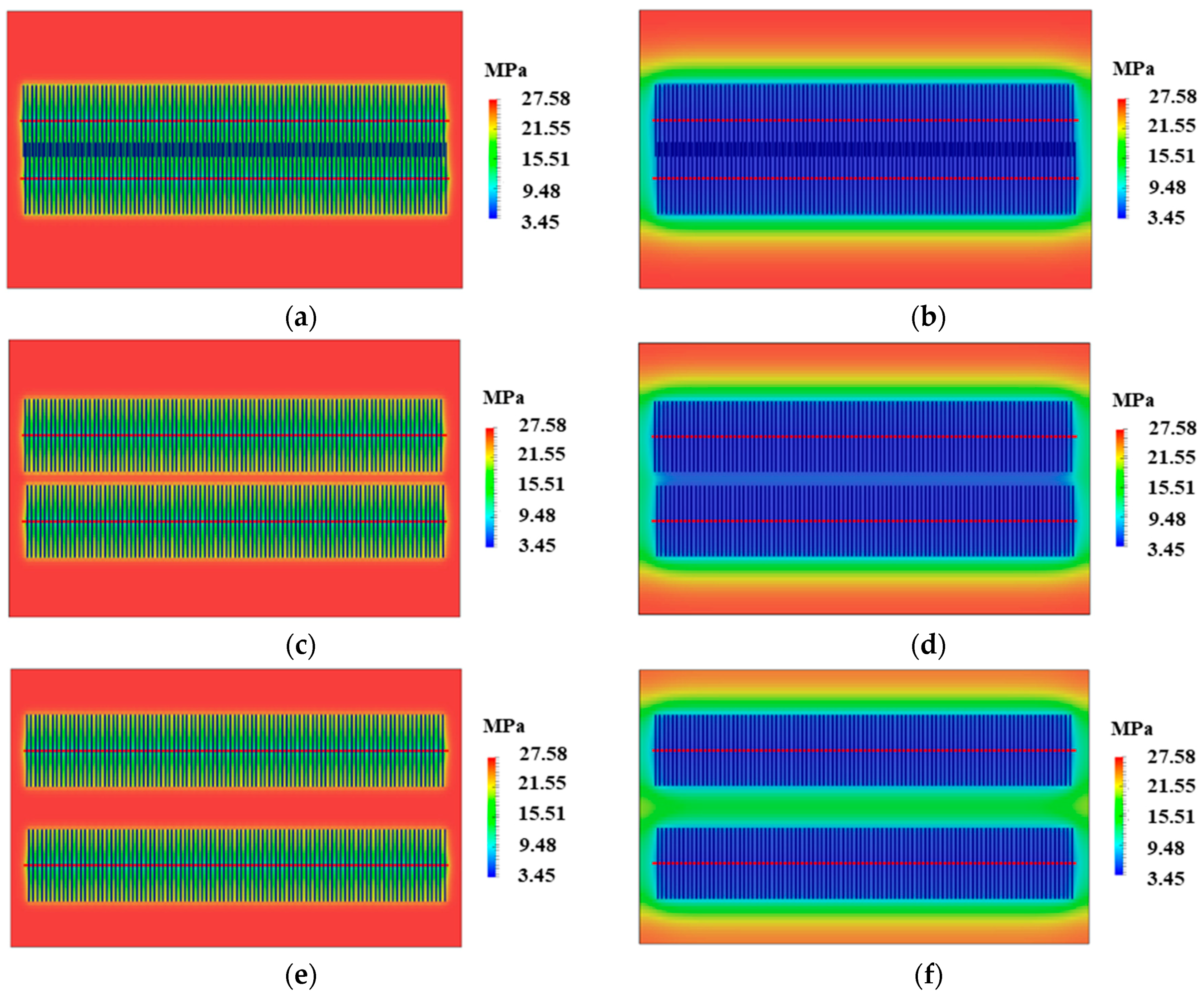
Figure 12.
Comparison of pressure distribution after 1 and 30 years of production under different well spacing without natural fractures: (a) After 1 year of production with well spacing 200 m; (b) After 30 years of production with well spacing 200 m; (c) After 1 year of production with well spacing 300 m; (d) After 30 years of production with well spacing 300 m; (e) After 1 year of production with well spacing 400 m; (f) After 30 years of production with well spacing 400 m.

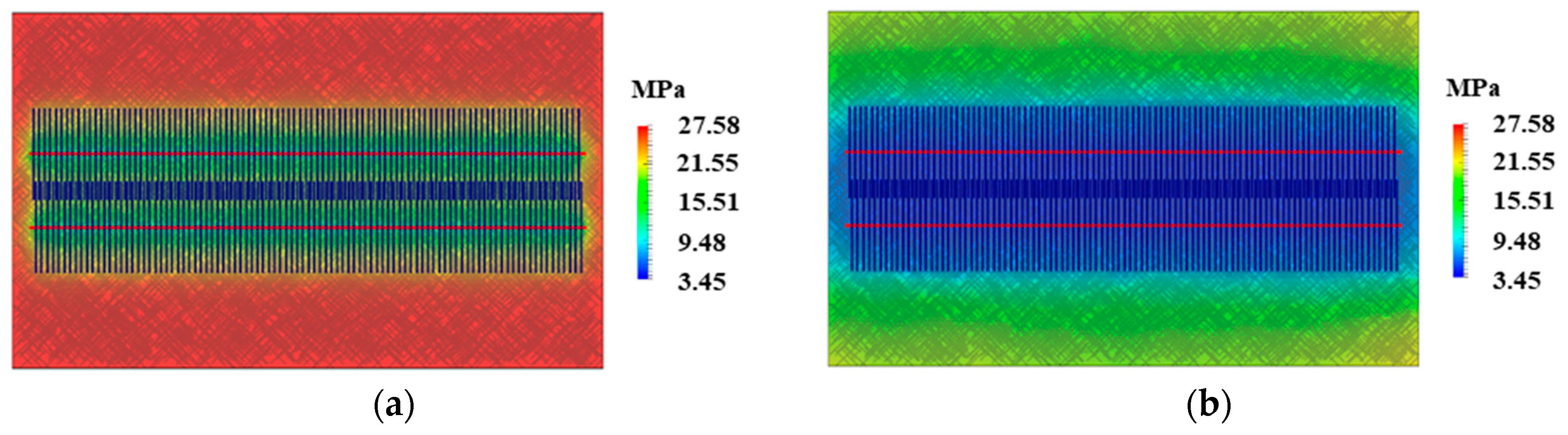
Figure 13.
Comparison of pressure distribution after one and 30 years of production under different well spacing with 10,000 natural fractures: (a) After one year of production with well spacing 200 m; (b) After 30 years of production with well spacing 200 m; (c) After one year of production with well spacing 300 m; (d) After 30 years of production with well spacing 300 m; (e) After one year of production with well spacing 400 m; (f) After 30 years of production with well spacing 400 m.


Table 1.
Reservoir and fracture properties used in the field-scale shale-gas model.
| Properties | Value | Unit |
|---|---|---|
| Initial reservoir pressure | 27.44 | MPa |
| Reservoir temperature | 54.5 | °C |
| Reservoir depth | 1889 | m |
| Residual water saturation | 20% | - |
| Porosity | 12.44% | - |
| Total compressibility | 3 × 10⁻⁷ | kPa−1 |
| Reference pressure for compressibility | 27.44 | MPa |
| Fracture aperture | 0.003 | m |
© 2019 by the authors. Licensee MDPI, Basel, Switzerland. This article is an open access article distributed under the terms and conditions of the Creative Commons Attribution (CC BY) license (http://creativecommons.org/licenses/by/4.0/).
Share and Cite
MDPI and ACS Style
Yu, W.; Hu, X.; Liu, M.; Wang, W. Investigation of the Effect of Natural Fractures on Multiple Shale-Gas Well Performance Using Non-Intrusive EDFM Technology. Energies 2019, 12, 932. https://doi.org/10.3390/en12050932
AMA Style
Yu W, Hu X, Liu M, Wang W. Investigation of the Effect of Natural Fractures on Multiple Shale-Gas Well Performance Using Non-Intrusive EDFM Technology. Energies. 2019; 12(5):932. https://doi.org/10.3390/en12050932
Chicago/Turabian StyleYu, Wei, Xiaohu Hu, Malin Liu, and Weihong Wang. 2019. "Investigation of the Effect of Natural Fractures on Multiple Shale-Gas Well Performance Using Non-Intrusive EDFM Technology" Energies 12, no. 5: 932. https://doi.org/10.3390/en12050932
Note that from the first issue of 2016, this journal uses article numbers instead of page numbers. See further details here.