Analysis of Different POD Processing Methods for SPIV-Measurements in Compressor Cascade Tip Leakage Flow


1
School of Energy and Power Engineering, Beihang University, Beijing 100191, China
2
Midea Corporate Research Center, Foshan 528300, China
*
Author to whom correspondence should be addressed.
Energies 2019, 12(6), 1021; https://doi.org/10.3390/en12061021
Submission received: 15 January 2019
/
Revised: 23 February 2019
/
Accepted: 11 March 2019
/
Published: 15 March 2019
(This article belongs to the Special Issue Fluid Flow and Heat Transfer)
Abstract
:Though the proper orthogonal decomposition (POD) method has been widely adopted in flow analysis, few publications have systematically studied the influence of different POD processing methods on the POD results. This paper investigates the effects of different decomposition regions and decomposition dimensionalities on POD decomposition and reconstruction concerning the tip flow in the compressor cascade. Stereoscopic particle image velocimetry (SPIV) measurements in the blade channel are addressed to obtain the original flow field. Through vortex core identification, development of the tip leakage vortex along the chord is described. Afterwards, each plane is energetically decomposed by POD. Using the identified vortex core center as the geometric center, the effects of different decomposition regions with respect to the vortex core are analyzed. Furthermore, the effects of different single velocity-components as well as their combination are compared. The effect of different decomposition regions on the mode 1 energy fraction mainly impacts the streamwise velocity component. Though the addition of W velocity component in the decomposition does change the spatial structures of high-order modes, it does not change the dynamic results of reconstruction using a finite number of POD modes. UV global analysis is better for capturing the kinetic physics of the tip leakage vortex (TLV) wandering.
1. Introduction
The efficiency, the pressure rise and the stable operating range are three prominent parameters for energy and power machinery, such as axial fans and compressors. The tip leakage flow (TLF), driven by the pressure difference between the pressure side and suction side of the blade in the tip region, plays a significant role in all three parameters mentioned above [1,2,3]. In recent years, the TLF, especially the tip leakage vortex (TLV), has been found to be an inherently unsteady flow phenomenon, with several distinct unsteady behaviors, including vortex wandering [4], vortex splitting [5,6] and vortex breakdown [7,8]. Previous studies showed that these unsteady behaviors not only have profound effects on the TLF mean characteristics, but also a close connection with some important flow phenomena such as rotating stall [9,10], rotating instability [11], oscillations of the TLV [12] and vortex shedding. Therefore, it is necessary to study the unsteady behaviors of the TLV to obtain a thorough knowledge of it.
Stereoscopic particle image velocimetry (SPIV) has been extensively employed to investigate the characteristics of the TLV for its ability to capture an instantaneous snapshot of tip flow structures at various scales [5,8,13,14]. Additionally, multiple averaging methods are also applied, among which the time-averaged method is frequently used. Several stochastic and deterministic characteristics of the TLV have been obtained through this method and statistics analysis [8,13,15]. Besides the simple averaging (ensemble averaging), some researchers employed a triple decomposition to extract the coherent wandering motion from the SPIV data [16]. Through this method, the TLV cores are collocated by linearly shifting the instantaneous core positions to the mean vortex core. This method was concluded to be superior to the simple averaging and recommended to analyze the characteristics of a concentrated vortex [17]. Oweis and Ceccio [14] used a vortex reconstruction method in which ideal Gaussian vortices were fitted to multiple vortices. As a result, they could reduce the effect of primary vortex wandering and reveal changes in flow variability that are masked by the vortex wandering process. However, the TLF is characterized by large-scale vortex and small-scale turbulence motion together. Many important information of unsteady flow behaviors associated with scale may be ignored using these averaging methods as a result.
The proper orthogonal decomposition (POD) method can decompose the examined flow field into orthogonal modes in space and identify the dominant mode based on energy rank [18,19]. It has been widely applied to both experimental and numerical data to identify some coherent structures, such as impeller flow [20], cylinder engine flow [21], wind turbine wake [22] and Jet and vortex actuator-induced flow [23]. Based on optimizing the mean square of the field variable, the POD method can extract flow structures of different scales. It is a promising key technique to analyze the flow structure, the kinematic and dynamic characteristics of the TLV in different length scales and energy levels. Unfortunately, there is a lack of use of the POD method to analyze the unsteady tip leakage flow. Recently, Li [24] introduced the POD method in turbine tip leakage flow analysis. Using the POD method, dominant flow modes governing the unsteady evolution in the tip region are successfully obtained. It is concluded that the POD method with advanced simulation approach can bring an interesting view of what can be done to better understand the leakage flow. Since the rapid development of numerical simulation and experimental techniques, the POD method is providing a new perspective about the tip flow physics.
However, spatial modes and energy distribution can in practice be obtained by different POD processing methods, such as using different decomposition dimensionalities [25,26] or different decomposition regions [27]. In the tip region, the streamwise velocity component is much stronger than the velocity components in the secondary flow direction. The TLV and wall boundary layer would introduce velocity deficits as well. Thus, the velocity and kinetic energy deviation would be quite diverse in different regions and different directions. This inevitably leads to different POD decomposition and reconstruction results using different decomposition regions and decomposition dimensionalities. Though the effects of many factors (POD algorithms [19], number of snapshots [25], analyzed flow variable [28]) have been assessed extensively, few publications have systematically studied the effects of decomposition regions and decomposition dimensionalities on the POD results. A clarification of the impacts of these two factors on POD decomposition and reconstruction results will help with a better and more efficient application of POD method in the TLF analysis.
In this paper, the effects of different decomposition regions and decomposition dimensionalities on POD decomposition and reconstruction of the tip flow are clarified. First, in the blade channel along a full chord length of a single compressor cascade, a SPIV measurement is addressed to obtain the original flow field for the POD decomposition and reconstruction. Combined with vortex core identification, development of the TLV along the chord is described. Then each plane is energetically decomposed and reconstructed using POD. In order to avoid the influence of main flow disturbance and extract more flow field structures associated with the TLV unsteady characteristics, POD decomposition regions are selected with caution. Using the identified vortex core as geometric center, the effects of different decomposition region with respect to the vortex core on POD decomposition are analyzed. Furthermore, the influences of different single velocity-components as well as their combination in POD decomposition are compared, so that to carry out a systematical studying on the effect of these two factors on the POD decomposition. Finally, combined with vortex statistical analysis, the impacts of decomposition dimensionalities in the reconstructed flow field are discussed. It is expected that findings presented in this paper will inspire other researchers who use POD to analyze the TLF.
This paper is organized as follows: firstly, the experimental apparatus and layout are introduced as follows; secondly, an overview of POD method and vortex core identification is given; in the following parts, the detailed comparison results are analyzed; the last section concludes this work.
2. Apparatus and Techniques
2.1. Experimental Facility and Test Conditions
The experiment is carried out in a low speed wind tunnel. The wind tunnel, as schematically shown in Figure 1, has a rectangular exit section of 250 mm by 120 mm (width × height). The test section of wind tunnel consists of a compressor cascade with seven blades, tip wall, hub wall and profile side walls as indicated in Figure 2. The parameters of the cascade and test conditions are listed in Table 1. During the experiment, the inlet velocity of the compressor cascade is kept at 30 m/s. At this velocity, the turbulence intensity in the mainstream is about 2.6%. We also measured the inlet boundary layer since it has a significant impact on the TLF roll-up procedure by interacting with the incoming main flow (Figure 3). The thickness of the boundary layer on the tip wall is about 3 mm.
2.2. SPIV Technique
An advanced commercial SPIV system is employed to measure the TLF field in the blade passage. As shown in Figure 2, the SPIV system is mainly composed of two 2048 × 2048 pixels, 12 bit frame-straddling based CCD cameras, a dual cavity Nd: YAG laser (200 mJ/pulse at a 15 Hz repetition rate) and a laser arm. The system is 2D-3C (two dimensional, three components) with two cameras located at different sides of the light sheet, which enables users to conduct the measurement of all three velocity components of a 3D flow.
The measurement cross sections are set to be perpendicular to the chordwise direction in the passage. 12 measurement locations along the chordwise direction (z-direction) are set, from L/c = 0 to L/c = 1.1 with an interval of 10% chord length, as shown in Figure 4. At each measurement location, at least 800 effective instantaneous images are recorded. The valid size of the cross section is about of 30 × 60 mm2, which covers nearly half spanwise range of the whole passage. The spatial resolution of the calibrated image is about 0.039 mm/pixel.
For the data processing, the inter-frame time is set to 10 μs based on the velocity of inlet flow and yields a maximum particle-image displacement of less than 8 pixels. A median-subtraction filter algorithm is applied to all the images to remove non-uniformities in the background light intensity. Subsequently, the particle-image is calculated by the software MicroVec V3 with the two-passes PIV interrogation algorithm. The dimensions of the interrogation region are 64 × 64 pixels in the first pass, and 32 × 32 pixels in the second pass. As a result, the spatial resolution of a single velocity vector is 1.26 mm × 1.26 mm. Once a vector field is calculated, vector validation algorithms must be used to eliminate spurious vectors. In the present work, the relative bias from the average vector is used as a post-processing criterion for eliminating questionable vectors, and the relative bias is set to be 50%.
2.3. Discussion of Uncertainties
The measurement error of the SPIV technique, including both random errors and bias errors, have been thoroughly discussed by many researchers [29,30,31,32,33,34,35,36]. Treated with caution during both the experiment and the data processing, random errors can be effectively eliminated. Bias errors depend crucially on the accuracy of particles displacement concerning the SPIV measurement in the compressor cascade. Among bias errors, the one caused by peak locking [30,32] should be dominated. In order to reduce this error, the least squares Gaussian sub-pixel fit for peak detection [5] is employed. Figure 5 illustrates the histogram of the displacement of the particles at the L/c = 1.0 measurement plane, which shows a well control of the peak locking effect during the SPIV experiments.
According to the analyses of Westerweel [34,36] and Raffle [30], the displacement errors of the in-plane component in the SPIV measurement is about 0.05 pixel. Taking other uncertainties (background noise, acceleration, velocity gradient) into consideration, the displacement errors of the in-plane component are estimated as 0.1 pixels.
Based on the theoretical analysis by Zang and Prasad [37], as shown in Equation (1) the error ratio between the out-of-plane and in-plane components depends on the camera included half angle:
where α is the camera included half angle; Ux, Uy and Uz are the uncertainties of the x, y and z velocity components. In this paper, this angle is set to 45°. Therefore, the displacement error of the out-of-plane component is 0.1 pixels as well.
The relative uncertainty of instantaneous velocity in the u-component can be estimated from the equation:
where K is converge factor related to measured velocity distribution characteristics. It is set to 2.576 for a 99% confidence interval. is the corresponding instantaneous velocity at the i, j grid node in the kth snapshot. Δ is error bound calculated by Equation (3). Likewise, the relative uncertainties of instantaneous velocity field in the v- and w-components can also be deduced:
where d is estimated displacement error, m is image magnification and dt is the inter-frame time.
The measurement uncertainties of the time-averaged velocity, contain both the statistical factor (type A uncertainty) and the factors unrelated with the statistical analysis (type B uncertainty).
Type A relative uncertainty of the time-averaged velocity can be estimated as [38]:
where uij is the time-averaged velocity in the u-component at the i, j grid node, N is the number of snapshots acquired, is the corresponding instantaneous velocity in the kth snapshot. Similarly, type A relative uncertainty of the time-averaged mean velocity in the other two components can also be deduced.
In the compressor cascade, the main factor contributing to the type B uncertainty of the time-averaged velocity() is the time-averaged of the instantaneous velocity deviation shown in Equation (2).
Thus, the combined standard relative uncertainty of the time-averaged velocity in the u-component can be given as:
The uncertainties of the time-averaged velocity can be calculated by the propagation of error formula:
where are the uncertainties of the time-averaged velocity in u-, v- and w-component.
The uncertainties of instantaneous velocity and time-averaged velocity are shown in Figure 6. Since the introduction of type A uncertainty, the uncertainty in the time-averaged velocity field is elevated. It can be seen that the uncertainty of time-averaged velocity is about 0.5–2% in the mainstream region, and it can achieve 6% near the tip wall. Moreover, it should be pointed out that in the tip region the accuracy of the in-plane components is about 0.5–3% and for the out-of-plane component is about 5–10%, and these results are not shown here for simplicity. Though the uncertainty of the out-of-plane component is higher, the statistical results are worthful for qualitative analyses of the unsteady characteristics in the compressor cascade, and constructive conclusions can be drawn from these results.
2.4. PODMethod
In this paper, a set of instantaneous SPIV measured velocity field V(k) (snapshots) with total number of K is decomposed into a linear combination of K spatial orthonormal basis function (POD modes, ) and the corresponding coefficients :
with the constraints that the following function is minimized [39]:
Considering the instantaneous snapshots V(k) made available from the SPIV measurement:
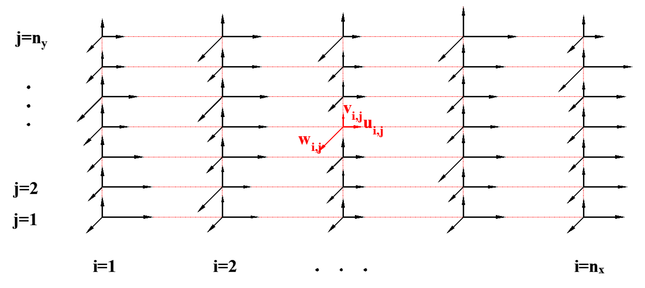
where k is the snapshot index, u, v, w are the velocity components in x, y and z direction respectively, i, j are the index of spatial position coordinates in the velocity distributions for a collocated setup, as illustrated in Figure 7.
Then the velocity component of every single snapshot V(k) is collated as following:
where nx × ny is the total number of the spatial positions.
The other two component-wise velocities are processed the same way and matrix V and matrix W are obtained, respectively. Then, simultaneously using both u and v velocity components and neglecting w, most researchers tend to define the spatial correlation matrix as follows [21,40]:
However, according to the works of Arányi [25] and Lengani [26], the results would be noticeably different if a multi-dimensional field is analyzed component-wise instead of globally. In this paper, we make a deeper quantitatively comparison of the decomposition results using different analysis dimensionalities to clarify whether decomposition dimensionalities impact the whole modes or just specific modes. Moreover, as the aim of most POD analyses is to reconstruct approximately the vector field, we also compare the reconstruction results based on two reconstruction criteria. Therefore, the spatial correlation matrices (C) are defined according to different analysis dimensionalities (AD) as shown in Table 2.
The minimization problem described in Equation (8) is realized by solving the eigenvalue problem of correlation matrix C:
where Eigenvalues are arranged in descending order according to the magnitude of eigenvalues, the basis function are obtained by projecting the snapshots onto the eigenvector .
The POD coefficients are obtained by projecting the snapshots onto the basis function and represents the energy contribution by the mth mode to the kth snapshot.
The K × K coefficient matrix :
The whole kinetic energy from all the snapshots captured by the mth mode is:
The fraction of the energy captured by the mth mode is:
By setting the amplitude of higher-order modes to zero, a low order flow field contains the most energetic modes is reconstructed:
where M is the reconstruction order less than K.
2.5. TLV Vortex Core Identification
The TLV is a concentrated vortex before splitting into several small vortices or breakdown. In order to identify the TLV core correctly, some criteria, such as Q criterion, λ2 criterion and Δ criterion, have been developed. The ability of the three criteria is similar to each other and none of them can be applied without error to all situations. Since the reduced −λ2 criterion has been employed in compressor TLV many times and can separates the TLV from the background high shear layer, here the reduced −λ2 criterion is employed [41]. This reduced criterion is effective to identify the TLV core and is given by Equation (17):
where x and y are coordinate axes in the measured cross section as demonstrated in Figure 4, and Vx and Vy are the velocity components in the corresponding directions. In this paper, zero threshold of λ2 is selected to identify the border of the TLV core.
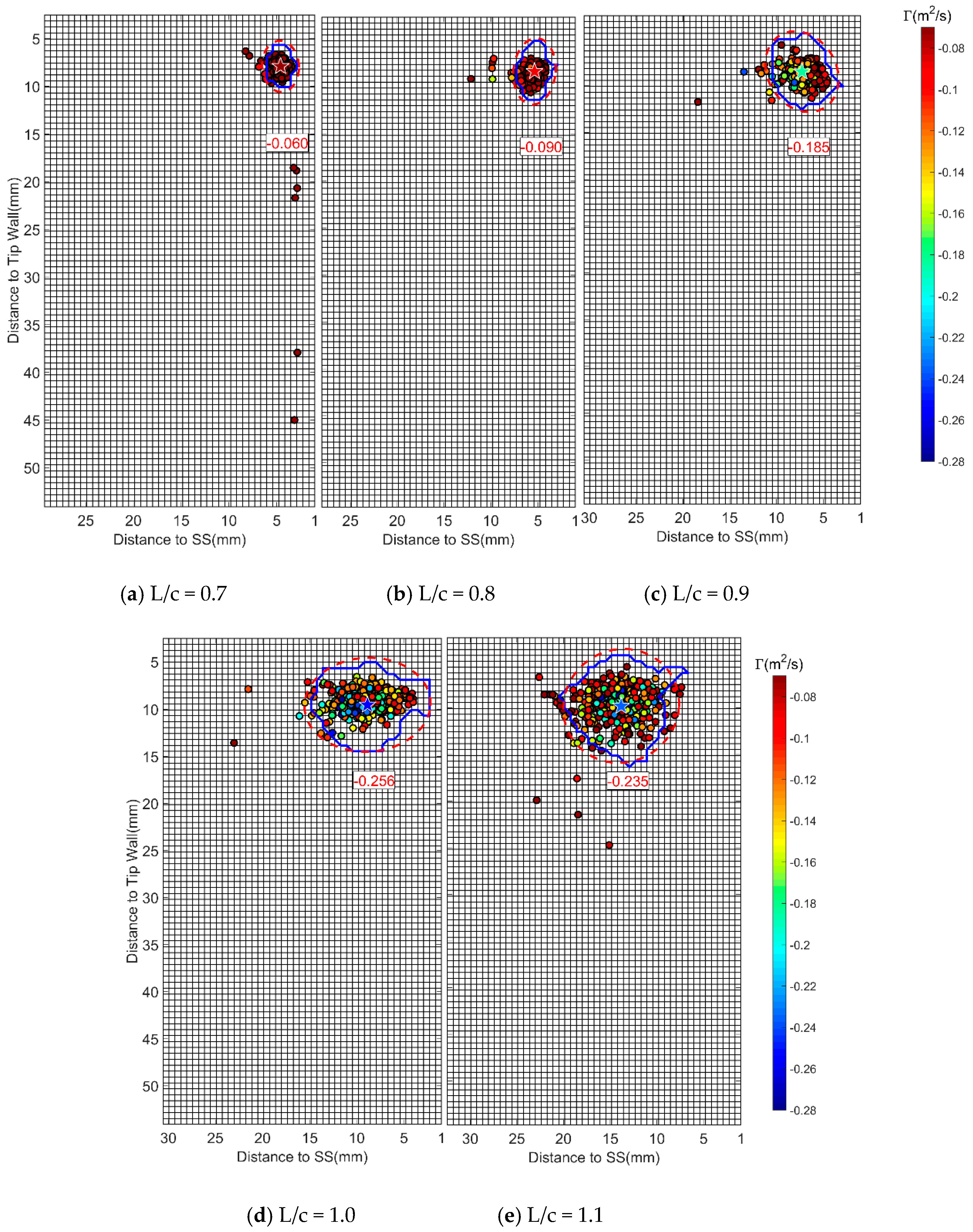
After the identification, the circulation and radius of the TLV core are quantitatively analyzed. The circulation, which represents the strength of the vortex, is obtained by calculating the line integral of velocity along the border. As shown in Figure 10, a red ellipse is used to fit the TLV core and the center and the radius of the TLV core are calculated from this fitting ellipse. The five-pointed star represents the center of the TLV core identified. The x-axis in the figure is the distance of the TLV core center to the blade suction surface. The y-axis is the distance of the center to the cascade tip wall. Detailed information about the identification program may be found in our previous study [42].
3. Results
3.1. Tip Flow Characteristics
Figure 8 lays out the time-averaged SPIV measurement results of the normalized streamwise velocity and λ2. The trajectory of the TLV cores can be seen clearly from the λ2 distribution. The concentrated TLV can be found after L/c = 0.5, which is an ambiguous result for the deficiency of SPIV spatial resolution in the z-direction.
As the TLV propagates downstream, the TLV core radius and the absolute value of vortex circulation expands rapidly (Quantitatively shown in Figure 9a). Figure 9a also quantitatively illustrates that the TLV moves slowly away from the blade tip suction surface in the x-direction (Schematically shown in Figure 9b from a bird’s eye view). In the y-direction, the TLV moves slowly away from the tip wall. The variance tendencies of the positions of the TLV in the time-averaged flow fields conform well with the SPIV results obtained in a laboratory-scale compressor at the design condition [5,6,42].
In Figure 10 the instantaneous vortex cores from L/c = 0.7 to L/c = 1.1 in all the SPIV snapshots are illustrated by single points. The vortex core center, border and border fitting ellipse of the time-averaged vortex are also shown in Figure 10 for comparison. At L/c = 0.7 most instantaneous TLV are near the core center of the time-averaged TLV. The position and circulation distribution of the TLV is in a relatively concentrated form. With the development of the TLV core to the trailing edge, the pitchwise and spanwise distribution range of the vortex expands. From L/c = 0.9 to L/c = 1.1, when the TLV is shedding form the blade suction side, wandering of the TLV cores becomes significantly stronger and the TLV motions cover a much wider area.
Figure 11 shows the standard deviation of normalized SPIV measured velocity. The flow velocity in every single snapshot is normalized by the inlet average velocity. The standard deviation is calculated as Equation (18) to show the unsteadiness of the TLV:
where Vsi is the instantaneous velocity in every single snapshot, is the time-averaged velocity.
As the vortex propagates downstream, the standard deviation of the normalized SPIV measured velocity near the TLV core increases. In this paper, the unsteadiness of the TLV is mainly originated from the TLV wandering as the vortex maintains a concentrate vortex and does not show any evidence of vortex splitting or breakdown.
The aforementioned experimental results demonstrated the main characteristics of the TLV. In the tip region, streamwise velocity component is much higher than velocity components in secondary flow directions. The TLV and wall boundary layers would introduce velocity deficits as well. Thus, in the compressor cascade, we should keep in mind that the decomposition regions and decomposition dimensionalities would have significant impacts while use the POD method to further analyze the TLV wandering characteristics. Therefore, the two factors should be investigated with caution to get reasonable POD results.
3.2. Effect of Decomposition Region on the Energy Fraction of Mode 1
Since the TLV is a concentrated vortex, to focus on the unsteady characteristics caused by the TLV wandering, circular decomposition regions are deliberately chosen. The decomposition regions are concentric circles with the time-averaged TLV core center as their common center. The radius Rdr of the decomposition regions are multiples of the time-averaged TLV core radius Rv. The borders of decomposition regions are shown as dotted line in Figure 12.
Figure 12 b shows the instantaneous TLV cores center, the time-averaged TLV core center and the time-averaged TLV core border. Figure 12c,d shows two instantaneous velocity snapshots chosen randomly. The minimum decomposition region (Rdr/Rv = 2) covers most instantaneous vortex cores centers. This selection of decomposition regions would keep most information of the TLV wandering and turbulence fluctuation around the TLV while removes the interference of the main flow. While the decomposition region converge to the TLV core center with Rdr/Rv reducing from 7 to 2, the effect of main flow on the POD results would be eliminated. Therefore, it is beneficial to extract more flow field structure associated with the unsteady wandering of the TLV and turbulence fluctuation around it.
Before the POD decomposition is performed, many researchers have addressed the difference in POD results between subtracting the time-averaged flow field and not subtracting [25,43,44]. As will be confirmed in the following, while the average is not removed, mode 1 is representative of the time-averaged velocity field. Since the POD modes are all orthogonal, the higher-order modes would be well estimates of the fluctuation. In this paper, the POD analysis is conducted without subtracting the average in the snapshots.
The energy rank is the first information provided by the POD eigenvalues λm [45]. Among the energy rank, the energy fraction of mode 1 is the most important. The total energy fraction of all other higher-order modes can be obtained by Equation (19):
Therefore, the energy fraction of mode 1 reflects the relative contribution of fluctuation to the whole energy of the flow field. The energy fraction of mode 1 can represent the level to which extent the instantaneous fields approach the time-averaged result.
From L/c = 0.6 to L/c = 1.1, as the fluid propagates downstream, the energy fraction of mode 1 decreases as shown in Figure 13. It should be noted that the results are from POD decompostion using three velocity vector components U, V and W simultaneously. The POD highlights that the flow posses a higher energy in fluctuation as the vortex propagates downstream, consistent with the results of the standard deviation previously observed in Figure 11. Figure 13 also shows that the deviation of mode 1 energy fraction between L/c = 0.6 and L/c = 1.1 becomes evident as the decomposition region converge to the TLV core. Indeed, the TLV experiences the process of vortex shedding from the blade suction side and wanders much stronger at the downstream near the trailing edge.
At the same chordwise position, as the decomposition region size decreases, the energy fraction of mode 1 decreases as well. The energy fraction of fine scale fluid structure, normally contained in the higher-order modes, is weakened by the introduction of main flow. It proves that the decomposition region chosen is beneficial to focus on the unsteady characteristics analysis of the TLV and turbulence fluctuation around it.
To further investigate the effect of decomposition regions on energy distribution, four more different analysis dimensionalities, such as UV global analysis, U component-wise analysis, V component-wise analysis and W component-wise analysis, are used.
3.3. Effect of Decompostion Dimensionalities on the Energy Fraction of Mode 1
Figure 14 demonstrates the energy fraction of mode 1 at different decomposition region sizes and different chord positions using four different analysis dimensionalities.
Note that the decomposition region sizes have marginal impact on the results associated with U component-wise analysis, V component-wise analysis and UV global analysis. However, the impact become considerable on the results associated with W component-wise and UVW global analysis while both of the results have the same variability tendency. This corresponding to the fact that the dominant flow direction is z-direction (streamwise) in this cascade while x-direction and y-direction are the secondary flow directions where velocity amplitude is relatively low.
As the flow travels downstream, the energy fraction of mode 1 decreases dramatically. From L/c = 0.6 to L/c = 1.1, the deviation of the energy fraction of mode 1 is nearly 10% in the U component-wise analysis, and higher than 20% in V component-wise analysis and UV global analysis as shown in Figure 14. While the W component is included, the deviation reduced to less than 5%. Therefore, the POD without the W component highlights the development of unsteady characteristics along the streamwise direction. The figure also shows that, using POD without the W component, mode 1 energy fraction at L/c = 0.9 deviate from that at L/c = 1.1 by twice as much as the deviation from L/c = 0.6 to L/c = 0.9. Near the trailing edge, the TLV is shedding from the blade suction surface, the instantaneous fields diverge considerably from the time-averaged result. UV global analysis captures this physics as the energy transferred from mode 1 expands significantly from L/c = 0.9 to L/c = 1.1.
Therefore, the effect of decomposition region on the mode 1 energy fraction mainly impacts the streamwise velocity component. When the decomposition region converges to the TLV core, the fraction of streamwise velocity deficit region increases, the impact of main flow with uniform streamwise velocity reduces, the unsteadiness caused by vortex wandering and turbulence fluctuation becomes evident.
Thus, the decomposition region size in the following work is all Rdr/Rv = 3, in order to extract more flow field structure associated with vortex wandering and turbulence fluctuation and to avoid the effect of main flow disturbance on POD. The results of five decomposition dimensionalities in the selected decomposition region are shown in Figure 15. It is interesting to note that the introduction of W velocity component also changes the absolute amplitude of mode 1 energy fraction. The amplitudes of mode 1 energy fraction are nearly equal in the results of UVW global analysis and W component-wise analysis and they are much higher than the result in the other three analyses.
Based on the aforementioned discussions, we can draw a conclusion that there is a marked difference among mode 1 energy fractions using different decomposition dimensionalities. If the aim of the analysis is to approximately reconstruct the flow field, the effects of decomposition dimensionalities on the spatial structures of POD modes and energy distribution should be urgent to clarify.
3.4. Effect of Decomposition Dimensionalities on POD Modes
3.4.1. Mode 1 and Its Relationship with the Time-Averaged Flow Field
To quantify the degree of similarity about two velocity vector fields, the relevance index Rp is used. Rp is obtained by projecting one velocity vector field onto another velocity vector field [43]:
where the denominator denotes the product of the L2 norm and the numerator is the inner product of two velocity fields. Rp = 0 means the two velocity field are orthogonal, Rp = 1 if the direction of two velocity vector field are identical, and Rp = −1 if the direction of two velocity vector field are exactly opposite.
The flow patterns of mode 1 from all three decomposition dimensionalities are excellent estimates of the time-averaged velocity field (shown in Figure 16). Moreover, the relevance indices Rp of all three mode 1 and the time-averaged velocity field are nearly 1, which also conforms this conclusion quantitatively. The results from other chordwise positions show the same correlation (not shown).
3.4.2. Higher-order Modes
Figure 17 reflects the relative contribution of the modes to the fluctuation energy of the flow field. The modes from W component-wise analysis show a distribution that the energy of the 3rd mode is similar to the 2nd mode. A completely different scenario characterized the POD energy distribution of other four decomposition dimensionalities, especially UVW global analysis. The energy content of the 2nd POD mode appears sensibly higher than that characterizing the 3rd mode.
Though the impact of W velocity component in mode 1 energy fraction is dominant as mentioned above, the addition of W velocity component in POD decomposition does not change the relative energy distribution of high-order modes. The 2nd and 3rd POD spatial modes from different decomposition dimensionalities have been checked. No matter which decomposition dimensionality used, two large well-defined vortex-like structures can be observed in the 2nd POD spatial modes (shown in Figure 16). However, the 3rd POD spatial modes are totally different from each other.
To further study the impact of decomposition dimensionalities in the high-order modes, the velocity correlation coefficients account for correlation of each mode from different decomposition dimensionalities are shown in Figure 18. The correlation coefficients of the 2nd POD mode are nearly 1, which verified that the 2nd POD mode is unaffected. The correlation coefficients of modes order higher than 3 are weak. In all, the three different decomposition dimensionalities lead to almost the same 2nd mode while significant difference can be observed in modes which order are higher than 2.
3.5. Effect of Decomposition Dimensionalities on POD Reconstruction
In the tip region, the flow is inherently unsteady. A single POD mode usually cannot bear a significant amount of energy and is not able to completely describe the original flow structures. An ensemble of POD modes is demanded to describe a particular dynamics. To study the dynamics of the TLV wandering, it is of great interest to analyze the vortex distribution characteristics with random noise being removed. In this section, to study the effect of different decomposition dimensionalities on the reconstructed flow field, the modes required to represent 95% energy of the original flow field and vortex distribution characteristics in the reconstructed flow field are compared.
3.5.1. Modes Required to Represent 95% Energy of the Original Flow Field
At the same chordwise position, modes required to represent 95% energy of the original flow field from UVW global analysis and W component-wise analysis are much less than that from other three processing methods. It also proves that the addition of W velocity component in the decomposition changes the energy fraction of every single mode and results in more energy gathering in the low-order modes.
From L/c = 0.6 to L/c = 1.1, an interesting feature in the POD reconstruction is that the modes required are dramatically increased using the U and V velocity components while maintain almost the same using the W velocity component (Figure 19). As the vortex propagates downstream, more and more modes are required to adequately represent the flow field in the x-direction and y-direction. Combining with the discussion in Section 3.3, UV global analysis is better for capturing the kinetic physics of the TLV because it is expected that more high-order modes will be present as the flow travels downstream due to vortex wandering and vortex shedding.
3.5.2. Effect of Decomposition Dimensionalities on the Vortex Distribution Characteristics
Two criteria of reconstructing flow field using POD modes is studied in this paper. Reconstruction using a finite number of modes [28,46,47] and reconstruction using modes that represent specific energy portion of the original flow field [45,48,49]. To compare the effect of decomposition dimensionalities on the vortex distribution characteristics in the reconstructed flow field, every single snapshot is reconstructed according to above two criteria.
Results from the reconstruction relying on the same retained energy in the reconstructed flow field are shown in Figure 20. Figure 21 quantitatively shows the proportion of the TLV core parameters. They together demonstrate the geometric and kinematic characteristics of the TLV in the reconstructed flow field. Since the modes required to reconstruct 95% energy of the original flow field is much less in UVW global analysis, the TLV shows more concentrated distribution characteristics in Figure 20. In the reconstructed flow field from UV global analysis and UV component analysis, the TLV cores are decentralized and have the similar distribution characteristics with the original flow field. The histogram of vortex distribution from UVW global analysis is symmetric that the mean value provides a good estimate for the center of the data. The histograms from UV global analysis and UV component analysis have the same shape, and are for a distribution that are skewed left. The reconstruction relying on the retained energy in the reconstructed flow field is sensitive to different decomposition dimensionalities.
Figure 22 and Figure 23 show the corresponding reconstruction results using the first ten modes. The vortex distributions in the reconstructed flow field using different decomposition dimensionalities show the same concentrated characteristics. The histograms of these three analyses have the same shape as well. Though the addition of W velocity component does change the spatial structures of high-order modes, it does not change the dynamic results of reconstruction using the same number of POD modes.
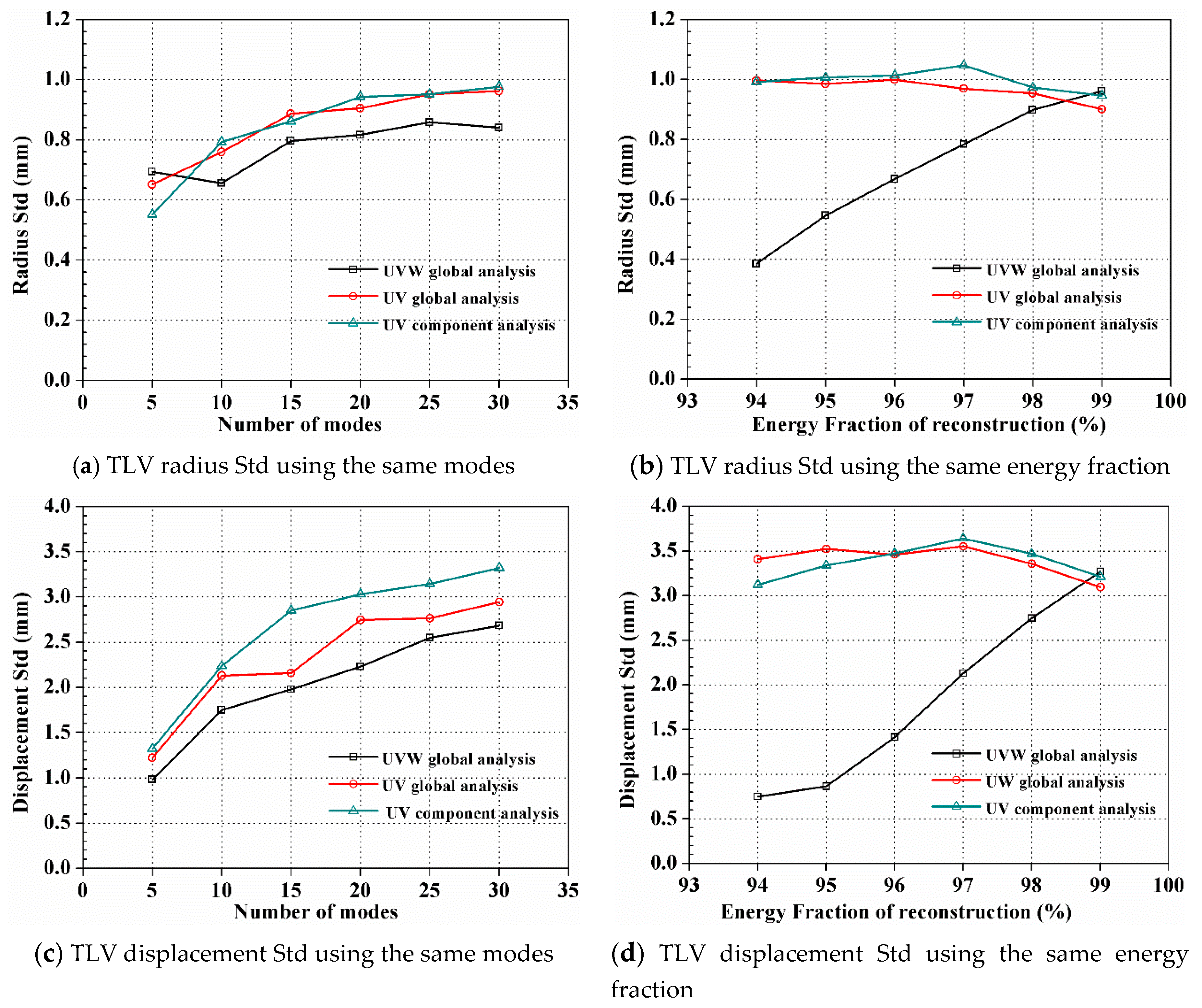
To further validate the conclusions drawn above, we checked the reconstruction results using different number of modes and different retained energy portions of the original flow field. The standard deviation of the TLV radius and displacement are chosen to quantitatively analysis the difference between the two reconstruction criteria. The results in Figure 24 confirm that reconstructions using the same modes number can obtain nearly the same vortex distribution characteristics while reconstructions relying on the same energy fraction would lead to totally different vortex distribution characteristics.
4. Conclusions
In this paper, based on the original tip flow field in the compressor cascade obtained by a SPIV measurement, the effects of different decomposition regions and decomposition dimensionalities on POD decomposition and reconstruction have been clarified. Several conclusions can be made as listed below:
- (1)
- From L/c = 0.9 to L/c = 1.1, when the TLV is shedding from the blade suction side, wandering of the TLV core becomes significantly stronger and the TLV motions cover a much wider area. As the TLV propagates downstream, the energy fraction of mode 1 decreases.
- (2)
- The decomposition region sizes have marginal impact on POD decomposition of secondary flow velocity. The impact become considerable on the results associated with W component-wise velocity.
- (3)
- For POD decomposition, using different dimensionalities, energy distributions and modes higher than 2 would be totally different. The dominant POD modes, such as the 1st and 2nd POD modes, stay unaffected. Using POD without the W component, mode 1 energy fraction at L/c = 0.9 deviate from that at L/c = 1.1 by twice as much as the deviation from L/c = 0.6 to L/c = 0.9.
- (4)
- The reconstruction relying on the retained energy in the reconstructed flow field is sensitive to different decomposition dimensionalities. The reconstruction using a finite number of POD modes is unaffected.
- (5)
- UV global analysis is better for capturing the kinetic physics of the TLV. As the flow travels downstream, more high-order modes with higher energy fraction will be present in UV global analysis, which is corresponding to the kinetic physics of the TLV that the unsteadiness of vortex wandering and vortex shedding becomes stronger.
Author Contributions
Conceptualization, L.S. methodology, L.S.; software, L.S.; validation, L.S.; formal analysis, L.S.; investigation, L.S.; resources, L.S.; data curation, L.S.; writing—original draft preparation, L.S.; writing—review and editing, H.M., L.W.; supervision, H.M.; funding acquisition, H.M.
Funding
This research was funded by the National Natural Science Foundation of China (Grant No. 51776011).
Conflicts of Interest
The authors declare no conflict of interest.
Nomenclature
| i,j | The index of the grid points in the velocity distributions |
| k | Snapshot index |
| L | SPIV measurement cross section chordwise position |
| c | Chord length |
| H | Span |
| p | Pitch length |
| Re | Reynolds number of the inlet flow |
| s | The vertical distance of test points to the wall. |
| Г | Circulation |
| ave | Time-averaged value |
| Std | Standard deviation |
| KE | Whole kinetic energy |
| ke | Energy of specific mode |
| Rp | Relevance index |
| M1 | Velocity vector fields |
| Rdr | Radius of the decomposition region |
| Rv | Radius of the TLV core |
| POD eigenvalues | |
| Ux, Uy, Uz | The uncertainties of the x, y and z velocity components |
| Δ | Error bound |
| K | Converge factor |
| The uncertainties of the time-averaged velocity in u-, v- and w-component | |
| POD mode | |
| AD | Analysis dimensionalities |
| C | Correlation matrices |
References
- Denton, J.D. Loss Mechanisms in Turbomachines; ASME 1993 International Gas Turbine and Aeroengine Congress and Exposition, 1993; American Society of Mechanical Engineers: New York, NY, USA, 1993. [Google Scholar]
- Storer, J.; Cumpsty, N. An approximate analysis and prediction method for tip clearance loss in axial compressors. J. Turbomach. 1994, 116, 648–656. [Google Scholar] [CrossRef]
- Adamczyk, J.; Celestina, M.; Greitzer, E. The Role of Tip Clearance in High-Speed Fan Stall; ASME 1991 International Gas Turbine and Aeroengine Congress and Exposition, 1991; American Society of Mechanical Engineers: New York, NY, USA, 1991. [Google Scholar]
- Straka, W.A.; Farrell, K.J. The effect of spatial wandering on experimental laser velocimeter measurements of the end-wall vortices in an axial-flow pump. Exp. Fluids 1992, 13, 163–170. [Google Scholar] [CrossRef]
- Liu, B.; Yu, X.; Liu, H.; Jiang, H.; Yuan, H.; Xu, Y. Application of SPIV in turbomachinery. Exp. Fluids 2006, 40, 621–642. [Google Scholar] [CrossRef]
- Xianjun, Y.; Baojie, L.; Haokang, J. Characteristics of the tip leakage vortex in a low-speed axial compressor. AIAA J. 2007, 45, 870–878. [Google Scholar] [CrossRef]
- Furukawa, M.; Inoue, M.; Saiki, K.; Yamada, K. The Role of Tip Leakage Vortex Breakdown in Compressor Rotor Aerodynamics. J. Turbomach. 1999, 121, 469–480. [Google Scholar] [CrossRef]
- Brandstetter, C.; Jüngst, M.; Schiffer, H.-P. Measurements of Radial Vortices, Spill Forward, and Vortex Breakdown in a Transonic Compressor. J. Turbomach. 2018, 140, 061004. [Google Scholar] [CrossRef]
- Day, I. The Fundamentals of Stall and Surge; Lecture series-van Kareman Institute for fluid dynamics; Von Kareman Institute for fluid dynamics: Rhode-Saint-Genèse, Belgium, 1996; pp. B1–B27. [Google Scholar]
- Inoue, M.; Kuroumaru, M.; Tanino, T.; Yoshida, S.; Furukawa, M. Comparative studies on short and long length-scale stall cell propagating in an axial compressor rotor. J. Turbomach. 2001, 123, 24–30. [Google Scholar] [CrossRef]
- Mailach, R.; Lehmann, I.; Vogeler, K. Rotating instabilities in an axial compressor originating from the fluctuating blade tip vortex. J. Turbomach. 2001, 123, 453–460. [Google Scholar] [CrossRef]
- Zierke, W.; Farrell, K.; Straka, W. Measurements of the tip clearance flow for a high-reynolds-number axial-flow rotor. J. Turbomach. 1995, 117, 522–532. [Google Scholar] [CrossRef]
- Liu, B.; An, G.; Yu, X.; Zhang, Z. Quantitative Evaluation of the Unsteady Behaviors of the Tip Leakage Vortex in a Subsonic Axial Compressor Rotor. Exp. Therm. Fluid Sci. 2016, 79, 154–167. [Google Scholar] [CrossRef]
- Oweis, G.F.; Ceccio, S.L. Instantaneous and time-averaged flow fields of multiple vortices in the tip region of a ducted propulsor. Exp. Fluids 2005, 38, 615–636. [Google Scholar] [CrossRef]
- Wu, H.; Tan, D.; Miorini, R.L.; Katz, J. Three-dimensional flow structures and associated turbulence in the tip region of a waterjet pump rotor blade. Exp. Fluids 2011, 51, 1721–1737. [Google Scholar] [CrossRef]
- Reynolds, W.; Hussain, A. The mechanics of an organized wave in turbulent shear flow. Part 3. Theoretical models and comparisons with experiments. J. Fluid Mech. 1972, 54, 263–288. [Google Scholar] [CrossRef]
- Van der Wall, B.G.; Richard, H. Analysis methodology for 3C-PIV data of rotary wing vortices. Exp. Fluids 2006, 40, 798–812. [Google Scholar] [CrossRef]
- Cordier, L. Proper Orthogonal Decomposition: An Overview; Lecture series 2002-04, 2003-03 and 2008-01 on post-processing of experimental and numerical data; Von Karman Institute for Fluid Dynamics: Rhode-Saint-Genèse, Belgium, 2008. [Google Scholar]
- Taira, K.; Brunton, S.L.; Dawson, S.T.M.; Rowley, C.W.; Colonius, T.; McKeon, B.J.; Schmidt, O.T.; Gordeyev, S.; Theofilis, V.; Ukeiley, L.S. Modal Analysis of Fluid Flows: An Overview. AIAA J. 2017, 55, 4013–4041. [Google Scholar] [CrossRef] [Green Version]
- Guo, R.; Li, R.; Zhang, R. Reconstruction and Prediction of Flow Field Fluctuation Intensity and Flow-Induced Noise in Impeller Domain of Jet Centrifugal Pump Using Gappy POD Method. Energies 2018, 12, 111. [Google Scholar] [CrossRef]
- El-Adawy, M.; Heikal, M.; A Aziz, A.; Adam, I.; Ismael, M.; Babiker, M.; Baharom, M.; Firmansyah; Abidin, E. On the Application of Proper Orthogonal Decomposition (POD) for In-Cylinder Flow Analysis. Energies 2018, 11, 2261. [Google Scholar] [CrossRef]
- Bastine, D.; Witha, B.; Wächter, M.; Peinke, J. Towards a Simplified DynamicWake Model Using POD Analysis. Energies 2015, 8, 895. [Google Scholar] [CrossRef]
- Cadirci, S.; Gunes, H. Proper Orthogonal Decomposition Analysis of JaVA Flows for Cross-Flow Conditions; ASME 2011 International Mechanical Engineering Congress and Exposition, 2011; American Society of Mechanical Engineers: New York, NY, USA, 2011; pp. 871–878. [Google Scholar]
- Li, H.; Su, X.; Yuan, X. Entropy Analysis of the Flat Tip Leakage Flow with Delayed Detached Eddy Simulation. Entropy 2018, 21, 21. [Google Scholar] [CrossRef]
- Arányi, P.; Janiga, G.; Zähringer, K.; Thévenin, D. Analysis of different POD methods for PIV-measurements in complex unsteady flows. Int. J. Heat Fluid Flow 2013, 43, 204–211. [Google Scholar] [CrossRef]
- Lengani, D.; Simoni, D.; Ubaldi, M.; Zunino, P. POD analysis of the unsteady behavior of a laminar separation bubble. Exp. Therm. Fluid Sci. 2014, 58, 70–79. [Google Scholar] [CrossRef]
- Maurel1, S.; Borée, J.; Lumley, J.L. Extended Proper Orthogonal Decomposition: Application to Jet/Vortex Interaction. Flow Turbul. Combust. 2001, 67, 125–136. [Google Scholar] [CrossRef]
- Kostas, J.; Soria, J.; Chong, M.S. A comparison between snapshot POD analysis of PIV velocity and vorticity data. Exp. Fluids 2005, 38, 146–160. [Google Scholar] [CrossRef]
- Perret, L.; Braud, P.; Fourment, C.; David, L.; Delville, J. 3-Component acceleration field measurement by dual-time stereoscopic particle image velocimetry. Exp. Fluids 2006, 40, 813–824. [Google Scholar] [CrossRef]
- Raffel, M.; Willert, C.E.; Scarano, F.; Kähler, C.J.; Wereley, S.T.; Kompenhans, J. Particle Image Velocimetry: A Practical Guide; Springer: Berlin, Germnay, 2018. [Google Scholar]
- Keane, R.D.; Adrian, R.J. Optimization of particle image velocimeters. I. Double pulsed systems. Meas. Sci. Technol. 1990, 1, 1202. [Google Scholar] [CrossRef]
- Huang, H.; Dabiri, D.; Gharib, M. On errors of digital particle image velocimetry. Meas. Sci. Technol. 1997, 8, 1427. [Google Scholar] [CrossRef]
- Hain, R.; Kähler, C. Fundamentals of multiframe particle image velocimetry (PIV). Exp. Fluids 2007, 42, 575–587. [Google Scholar] [CrossRef]
- Westerweel, J. Theoretical analysis of the measurement precision in particle image velocimetry. Exp. Fluids 2000, 29, S003–S012. [Google Scholar] [CrossRef]
- Boillot, A.; Prasad, A. Optimization procedure for pulse separation in cross-correlation PIV. Exp. Fluids 1996, 21, 87–93. [Google Scholar] [CrossRef]
- Westerweel, J. Fundamentals of digital particle image velocimetry. Meas. Sci. Technol. 1997, 8, 1379. [Google Scholar] [CrossRef]
- Zang, W.; Prasad, A.K. Performance evaluation of a Scheimpflug stereocamera for particle image velocimetry. Appl. Opt. 1997, 36, 8738–8744. [Google Scholar] [CrossRef] [PubMed]
- Cantrell, C.D. Modern Mathematical Methods for Physicists and Engineers; Cambridge University Press: Cambridge, UK, 2000. [Google Scholar]
- Lumley, J. The Structure of Inhomogeneous Turbulence; Atmospheric Turbulence and Wave Propagation, Nauka: Moscow, Russia, 1967; pp. 166–178. [Google Scholar]
- El-Adawy, M.; Heikal, M.R.; A Aziz, A.R.; Siddiqui, M.I.; Munir, S. Characterization of the Inlet Port Flow under Steady-State Conditions Using PIV and POD. Energies 2017, 10, 1950. [Google Scholar] [CrossRef]
- Jeong, J.; Hussain, F. On the identification of a vortex. J. Fluid Mech. 2006, 285, 69–94. [Google Scholar] [CrossRef]
- Ma, H.; Wei, W.; Ottavy, X. Experimental investigation of flow field in a laboratory-scale compressor. Chin. J. Aeronaut. 2017, 30, 31–46. [Google Scholar] [CrossRef]
- Hao, C.; David, L.R.; Volker, S. On the use and interpretation of proper orthogonal decomposition of in-cylinder engine flows. Meas. Sci. Technol. 2012, 23, 085302. [Google Scholar]
- Liu, K.; Haworth, D.C. Development and Assessment of POD for Analysis of Turbulent Flow in Piston Engines; SAE International: Warrendale, PA, USA, 2011. [Google Scholar]
- Lengani, D.; Simoni, D.; Pichler, R.; Sandberg, R.; Michelassi, V.; Bertini, F. On the Identification and Decomposition of the Unsteady Losses in a Turbine Cascade; ASME Turbo Expo 2018: Turbomachinery Technical Conference and Exposition, 2018; American Society of Mechanical Engineers: New York, NY, USA, 2018; p. V02AT45A013. [Google Scholar]
- Hossain, M.S.; Bergstrom, D.J.; Chen, X.B. Visualisation and analysis of large-scale vortex structures in three-dimensional turbulent lid-driven cavity flow. J. Turbul. 2015, 16, 901–924. [Google Scholar] [CrossRef]
- Hellström, L.H.O.; Ganapathisubramani, B.; Smits, A.J. The evolution of large-scale motions in turbulent pipe flow. J. Fluid Mech. 2015, 779, 701–715. [Google Scholar] [CrossRef] [Green Version]
- Raiola, M.; Discetti, S.; Ianiro, A. On PIV random error minimization with optimal POD-based low-order reconstruction. Exp. Fluids 2015, 56, 75. [Google Scholar] [CrossRef]
- Chen, H.; Reuss, D.L.; Hung, D.L.S.; Sick, V. A practical guide for using proper orthogonal decomposition in engine research. Int. J. Engine Res. 2012, 14, 307–319. [Google Scholar] [CrossRef]
Figure 1.
Schematic of the low-speed cascade wind tunnel.

Figure 2.
Schematic of compressor cascade and the SPIV measurement configuration.

Figure 3.
Velocity profiles at the hub and tip walls. Note that the y-axis is the vertical distance of test points to the wall.
Figure 3.
Velocity profiles at the hub and tip walls. Note that the y-axis is the vertical distance of test points to the wall.
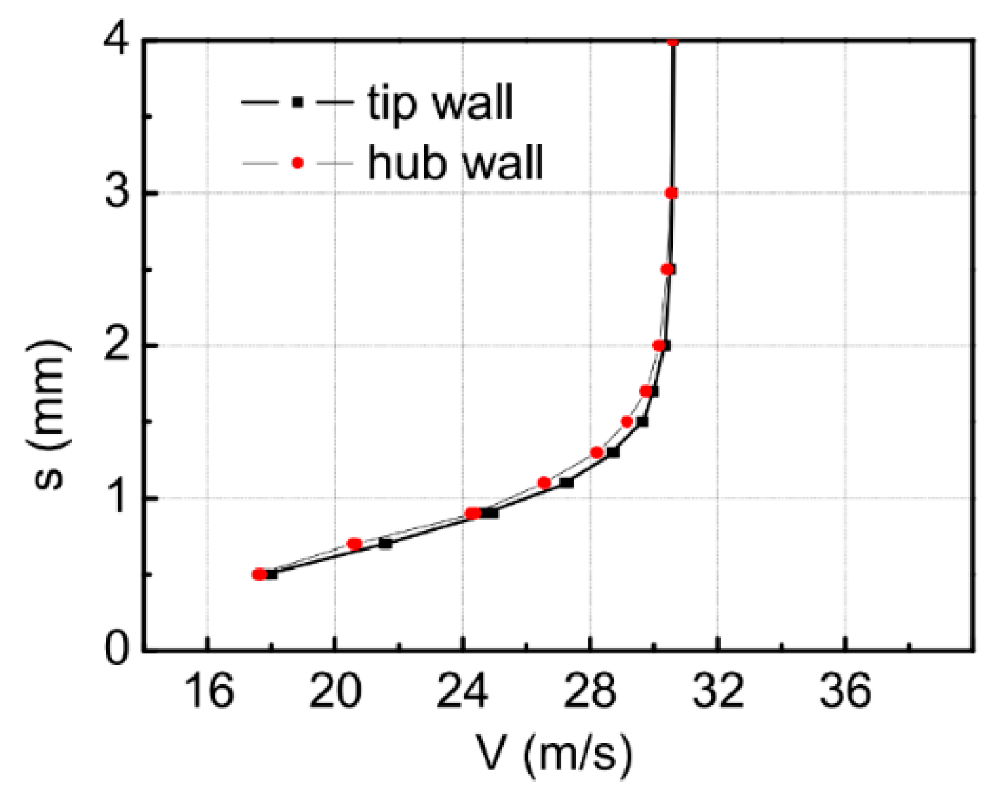
Figure 4.
Layout of SPIV measurement cross-sections.

Figure 5.
Histograms of the measured particle-image displacement at L/c = 1.0. (79,680 vectors in total, dx and dy are the particle-image displacements in the x and y directions).
Figure 5.
Histograms of the measured particle-image displacement at L/c = 1.0. (79,680 vectors in total, dx and dy are the particle-image displacements in the x and y directions).

Figure 6.
Distribution of measurement relative uncertainties in percentage terms at L/c = 1.0, (a) the instantaneous velocity, (b) the time-averaged velocity. The velocity is the resultant velocity of components in the x-, y- and z- direction.
Figure 6.
Distribution of measurement relative uncertainties in percentage terms at L/c = 1.0, (a) the instantaneous velocity, (b) the time-averaged velocity. The velocity is the resultant velocity of components in the x-, y- and z- direction.

Figure 7.
Example of discrete SPIV data on a uniform collocated grid.

Figure 8.
Combined maps of time-averaged SPIV measurement results in the blade passage. (a) Normalized Streamwise Velocity; (b) λ2. The red dash lines on both maps sketch the trajectory of the TLV cores.
Figure 8.
Combined maps of time-averaged SPIV measurement results in the blade passage. (a) Normalized Streamwise Velocity; (b) λ2. The red dash lines on both maps sketch the trajectory of the TLV cores.


Figure 9.
(a) Statistics of identified TLV time-averaged parameters; (b) Schematic of TLV core trajectory. Normalized pitch distance is the distance of the TLV core center to the blade suction surface in the x-direction normalized by the span, normalized span distance is the distance of the TLV core center to the tip wall in the y-direction normalized by the span.
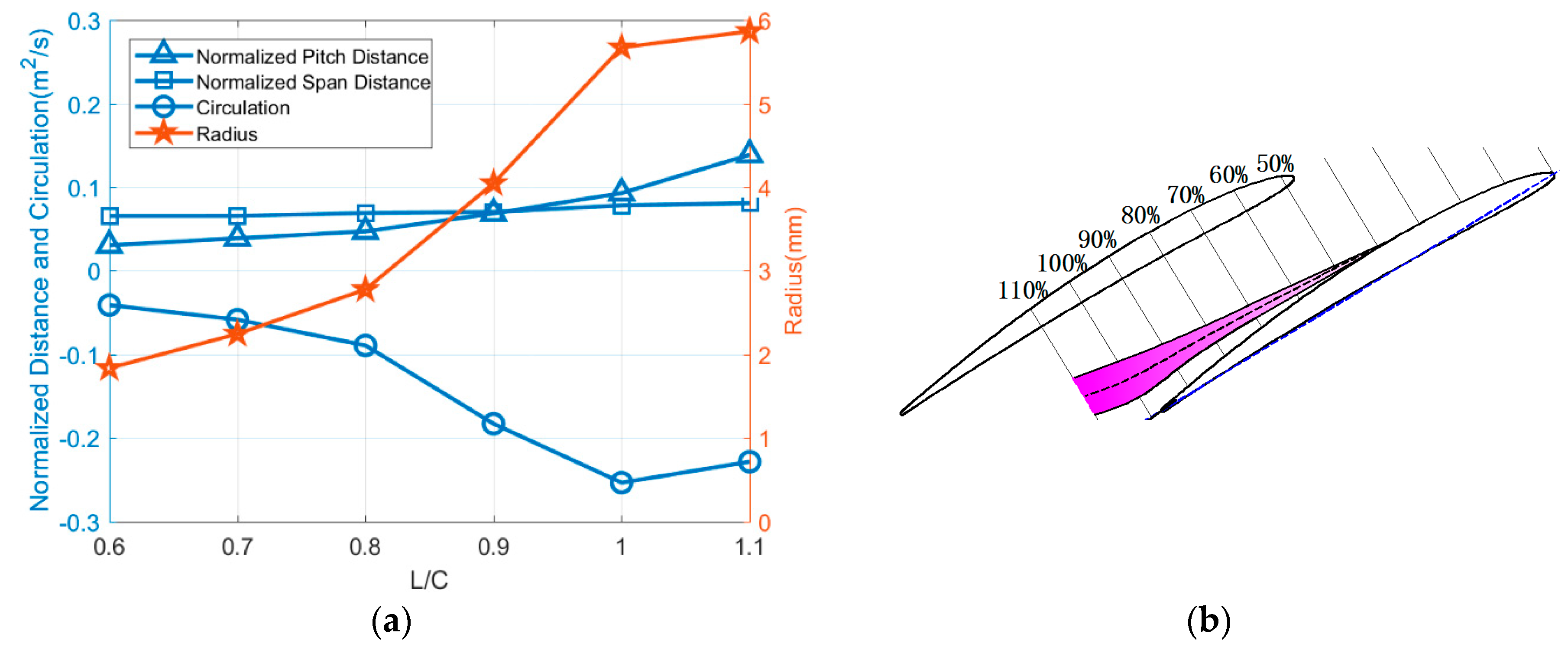
Figure 10.
Statistical distribution of the locations, area and circulation of identified TLV cores. The color of the points shows the vortex circulation.
Figure 10.
Statistical distribution of the locations, area and circulation of identified TLV cores. The color of the points shows the vortex circulation.

Figure 11.
Standard deviation of normalized SPIV measured velocity in the blade passage. The velocity is the resultant velocity of components in the x-, y- and z- direction.
Figure 11.
Standard deviation of normalized SPIV measured velocity in the blade passage. The velocity is the resultant velocity of components in the x-, y- and z- direction.

Figure 12.
Decomposition regions at L/c = 1.1.
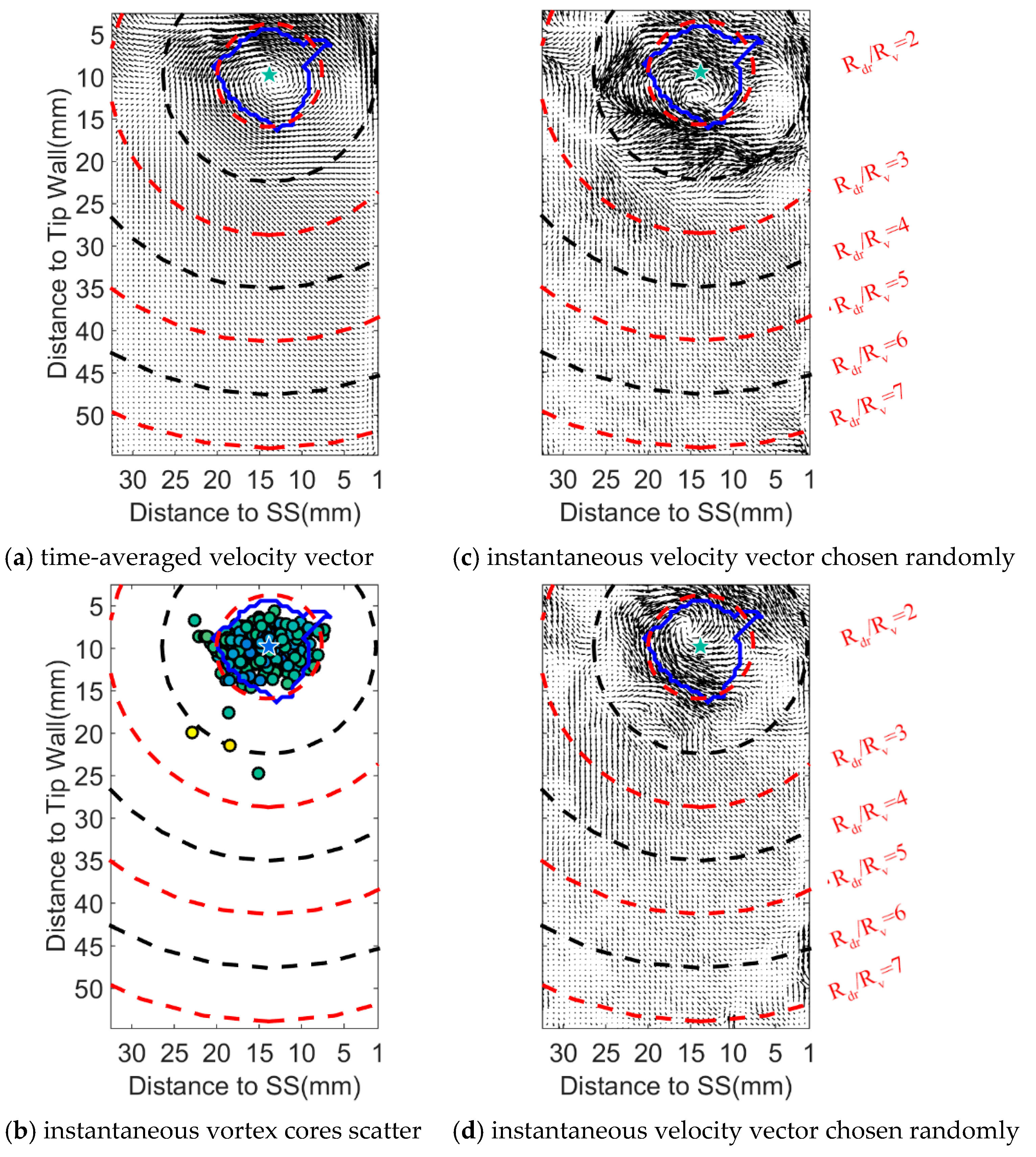
Figure 13.
Mode 1 energy fraction at different decomposition region sizes and different chord position.
Figure 13.
Mode 1 energy fraction at different decomposition region sizes and different chord position.

Figure 14.
Mode 1 energy fraction at different decomposition region sizes and different chord position.
Figure 14.
Mode 1 energy fraction at different decomposition region sizes and different chord position.

Figure 15.
Mode 1 energy fraction at different retained dimensionalities and different chord position when the decomposition region size is Rdr/Rv = 3.
Figure 15.
Mode 1 energy fraction at different retained dimensionalities and different chord position when the decomposition region size is Rdr/Rv = 3.

Figure 16.
Time-averaged velocity vector field and spatial structures of mode 1, 2 and 3 in UV global analysis at L/c = 1.1.For simplicity, the spatial structures of UVW global analysis and UV component analysis have not shown.
Figure 16.
Time-averaged velocity vector field and spatial structures of mode 1, 2 and 3 in UV global analysis at L/c = 1.1.For simplicity, the spatial structures of UVW global analysis and UV component analysis have not shown.

Figure 17.
Relative energy of modes higher than 2 from all five different decomposition dimensionalities.
Figure 17.
Relative energy of modes higher than 2 from all five different decomposition dimensionalities.

Figure 18.
The velocity correlation of high-order modes from different decomposition dimensionalities at L/c = 1.1.
Figure 18.
The velocity correlation of high-order modes from different decomposition dimensionalities at L/c = 1.1.

Figure 19.
The modes required to represent 95% energy of the original flow field using five different POD processing methods.
Figure 19.
The modes required to represent 95% energy of the original flow field using five different POD processing methods.

Figure 20.
Vortex distribution in the reconstructed flow field that represents 95% energy of the original flow field at L/c = 1.1. The color of the points shows the vortex circulation.
Figure 20.
Vortex distribution in the reconstructed flow field that represents 95% energy of the original flow field at L/c = 1.1. The color of the points shows the vortex circulation.
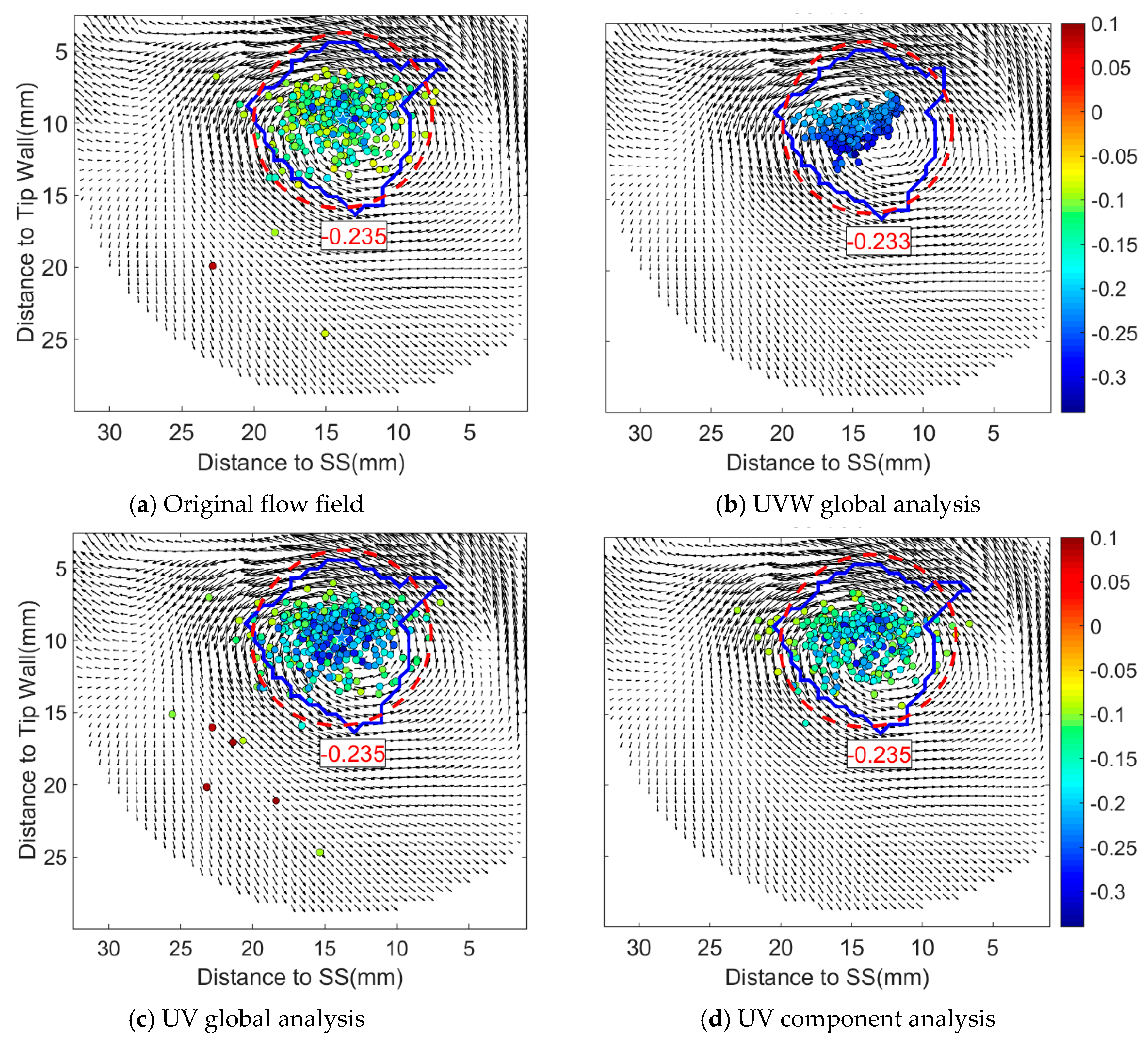
Figure 21.
Statistics of instantaneous reconstructed flow field that represents 95% energy fraction of the original flow field at L/c = 1.1. Note that the parameters from left side to the right are the distance of the TLV core center to the suction side, the distance of the TLV core center to the cascade tip wall, the TLV vortex circulation, the TLV vortex core radius and the distance of instantaneous TLV core center to the time-averaged TLV core center respectively. ‘std’ and ‘ave’ in the figure show the standard deviation and time-averaged value respectively.

Figure 22.
Vortex distribution from reconstructed flow field using first 10 modes at L/c = 1.1.


Figure 23.
Statistics of instantaneous reconstructed flow field using first 10 modes at L/c = 1.1.

Figure 24.
Comparison of reconstruction results based on the two reconstruction criteria at L/c = 1.1. The displacement is the distance of instantaneous TLV core center to the time-averaged TLV core center.
Figure 24.
Comparison of reconstruction results based on the two reconstruction criteria at L/c = 1.1. The displacement is the distance of instantaneous TLV core center to the time-averaged TLV core center.


Table 1.
Cascade parameters and test condition.
| Items | Details |
|---|---|
| Number of blades, N | 7 |
| Chord length, c | 126.8 mm |
| Span, H | 120 mm |
| Pitch, p | 72 mm |
| Reynolds No., Re | 2.81 × 10⁵ |
| Incidence angle | 0 degree |
| Tip clearance/c | 5% |
Table 2.
Five spatial correlation matrices for different decomposition dimensionalities.
| Processing Methods | Global Analysis | Component-Wise Analysis | |||
|---|---|---|---|---|---|
| AD | UVW-simultaneously | UV-simultaneously | U | V | W |
| C | |||||
© 2019 by the authors. Licensee MDPI, Basel, Switzerland. This article is an open access article distributed under the terms and conditions of the Creative Commons Attribution (CC BY) license (http://creativecommons.org/licenses/by/4.0/).
Share and Cite
MDPI and ACS Style
Shi, L.; Ma, H.; Wang, L. Analysis of Different POD Processing Methods for SPIV-Measurements in Compressor Cascade Tip Leakage Flow. Energies 2019, 12, 1021. https://doi.org/10.3390/en12061021
AMA Style
Shi L, Ma H, Wang L. Analysis of Different POD Processing Methods for SPIV-Measurements in Compressor Cascade Tip Leakage Flow. Energies. 2019; 12(6):1021. https://doi.org/10.3390/en12061021
Chicago/Turabian StyleShi, Lei, Hongwei Ma, and Lixiang Wang. 2019. "Analysis of Different POD Processing Methods for SPIV-Measurements in Compressor Cascade Tip Leakage Flow" Energies 12, no. 6: 1021. https://doi.org/10.3390/en12061021
Note that from the first issue of 2016, this journal uses article numbers instead of page numbers. See further details here.