Rotor Loading Characteristics of a Full-Scale Tidal Turbine

Abstract

Tidal turbines are subject to highly dynamic mechanical loading through operation in some of the most energetic waters. If these loads cannot be accurately quantified at the design stage, turbine developers run the risk of a major failure, or must choose to conservatively over-engineer the device at additional cost. Both of these scenarios have consequences on the expected return from the project. Despite an extensive amount of research on the mechanical loading of model scale tidal turbines, very little is known from full-scale devices operating in real sea conditions. This paper addresses this by reporting on the rotor loads measured on a 400 kW tidal turbine. The results obtained during ebb tidal conditions were found to agree well with theoretical predictions of rotor loading, but the measurements during flood were lower than expected. This is believed to be due to a disturbance in the approaching flood flow created by the turbine frame geometry, and, to a lesser extent, the non-typical vertical flow profile during this tidal phase. These findings outline the necessity to quantify the characteristics of the turbulent flows at sea sites during the entire tidal cycle to ensure the long-term integrity of the deployed tidal turbines.

1. Introduction

Survivability of tidal stream turbines is dependent on their ability to withstand recurrent unsteady loadings due to the turbulent approach flow. At energetic tidal stream sites, there are various sources that contribute to the harsh marine flow conditions that turbines encounter, including turbulence in the fast-flowing tidal flow, waves and bathymetry-induced effects. Complexity in parameterising marine environments in which turbines operate arises from the fact that the flow conditions developed at any potential deployment site are completely unique as, even within a narrow region, the flow properties can vary dramatically both spatially [1] and temporally [2]. This uncertainty constitutes a huge challenge for tidal turbine developers as the mechanical loading that their devices will be subject to is dependent on the local conditions at the deployment site, demanding bespoke design modifications to ensure long-term integrity.

Turbulence in a tidal flow can be mainly characterised by two parameters, namely turbulence intensity, $I_x$, that relates the root-mean-square of velocity fluctuations to the mean velocity; and turbulence length scale, $L_u$, that accounts for the spatial dimensions of the largest scales in the flow. Turbulence intensity is often considered as the key parameter related to the variation of performance and structural loading of tidal turbines [3,4]. However, during an extensive experimental campaign, Blackmore et al. [5] evidenced that the turbulence length scale has the greatest impact on the turbine loading. At most tidal sites suitable for the deployment of bottom-fixed tidal turbines, the flow conditions can be deemed relatively shallow and hence the length scale of the largest flow structures are constrained by the water depth H. Milne et al. [6] observed at the Sound of Islay (United Kingdom) the measured turbulent length scales across the water column can be well approximated as $L_u\approx \sqrt{zH}$, where z is the relative elevation from the sea bottom [7]. Therefore, the impact of the dominant flow scales responsible for loadings oscillations on a turbine may be expected to vary depending on the ratio of the water depth, specifically with $L_u$, to the turbine diameter.

In the assessment of the tidal energy resource at a given site, it is fundamental to measure the temporal variation of the velocity profile across the water depth during ebb and flood tides. A common assumption of the vertical velocity distribution is that due to bottom shear, a logarithmic profile is developed. As this sheared profile depends on the bed roughness and bulk flow velocity, it can change considerably during tidal cycles. Lewis et al. [2] found that a 1/7th power law can be assumed as the most likely velocity distribution based on measurements taken at two different sites in the UK, but also showed that the profile can follow power-law distributions with exponents 1/5 or 1/9 during other periods of time. Togneri and Masters [8] observed at Ramsey Sound (Wales, UK) the velocity profile during ebb tides again followed a power-law distribution over the entire water column, while during flood tides the logarithmic distribution of velocities was observed over the bottom half of the water column only, with the remainder being almost uniform up to the free-surface. Evans et al. [1] further characterised Ramsey Sound evidencing a large variability of the tidal energy resource that can be extracted within relatively short distances as a result of the local flow characteristic variations. Parkinson and Collier [9] reported on field measurements at the European Marine Energy Centre (EMEC) in Scotland (UK), finding similar observations of drastic temporal changes in the approach flow distribution during ebb and flood tides. Garcia-Novo and Yukasu [10] observed that the flow at Naru Strait (Japan) features a remarkable variation between ebb and flood tidal conditions, with those during the former more energetic and uniformly distributed, while during flood the velocities were more scattered with reduced mean velocity value compared to ebb.

To date, most of the reported research on the mechanical loading on tidal turbines consider prototype-scale devices tested in laboratory facilities. Mycek et al. [3] studied the impact of different turbulent flow conditions in the loadings and wake of a single turbine. Blackmore et al. [5] quantified the effect of various turbulence intensities and length scales on the thrust and bending moment on a single turbine and revealed that larger turbulence length scales increase load oscillations. Milne et al. [6] studied the variation of bending moment oscillations inducing single periodic loadings on a single turbine with various amplitudes and found that dynamic stall triggered load unsteadiness. Payne et al. [11] investigated the spectral distribution of blade loadings on a single turbine operating under low and high turbulent conditions, finding that ambient turbulence largely affects the loads spectra as blade passing frequency-related phenomena smoothed.

Prototype-scale devices in open sea conditions have been tested to a lesser extent due to the inherent up-scaling challenges, e.g., Jeffcoate et al. [12] tested a 4 m diameter, 50 kW turbine and Frost et al. [13] compared the performance of a 1.5 m diameter turbine in both towing tank tests and at a tidal site. It should be noted that there are a significant number of engineering challenges when moving from small-scale prototype tests in controlled conditions to full-scale turbine deployments in open sea sites, particularly in terms of obtaining reliable device and environmental measurements. Thus, a degree of increased uncertainty should be expected for full-scale testing [14]. The up-scaling process has only been achieved by a handful of turbine developers, and consequently very few publications have reported on the testing of full-scale devices, e.g., Parkinson and Collier [9] reported data on the performance, bending moments and fatigue loadings on a 1 MW tidal turbine deployment.

In this work, the mechanical loading on the rotor of a full-scale, grid-connected tidal turbine deployed at Ramsey Sound (Wales, UK) is reported, obtained from operational periods in both ebb and flood tidal conditions. This was a first-of-kind deployment in Wales, and a step towards meeting the target set by the Welsh Government of capturing at least 10% of the potential tidal stream and wave energy off the Welsh coastline by 2025 [15]. The paper is structured as follows: Section 2 introduces the Ramsey Sound deployment site and its tidal resource characteristics; Section 3 describes the turbine and its operational principles, as well as the instrumentation relevant to this work; while Section 4 reports on the measured flow conditions (Section 4.1) and the rotor loading on the turbine during periods of operation in Section 4.2. The analysis considers both the mean (Section 4.3) and dynamic (Section 4.4) rotor loading with respect to the unsteady approach flow. The main conclusions from this analysis are summarised in Section 5.

2. Location

2.1. Ramsey Sound

Ramsey Sound is a sea channel located off the south west coast of Wales, UK, separating Ramsey island from the Welsh mainland. The narrowing of the channel leads to energetic tidal currents flowing through the site, northwards on flood tides and southwards on ebb tides. This, combined with a wave climate that is sheltered by Ramsey island, has resulted in considerable interest in the site for the development of tidal stream energy.

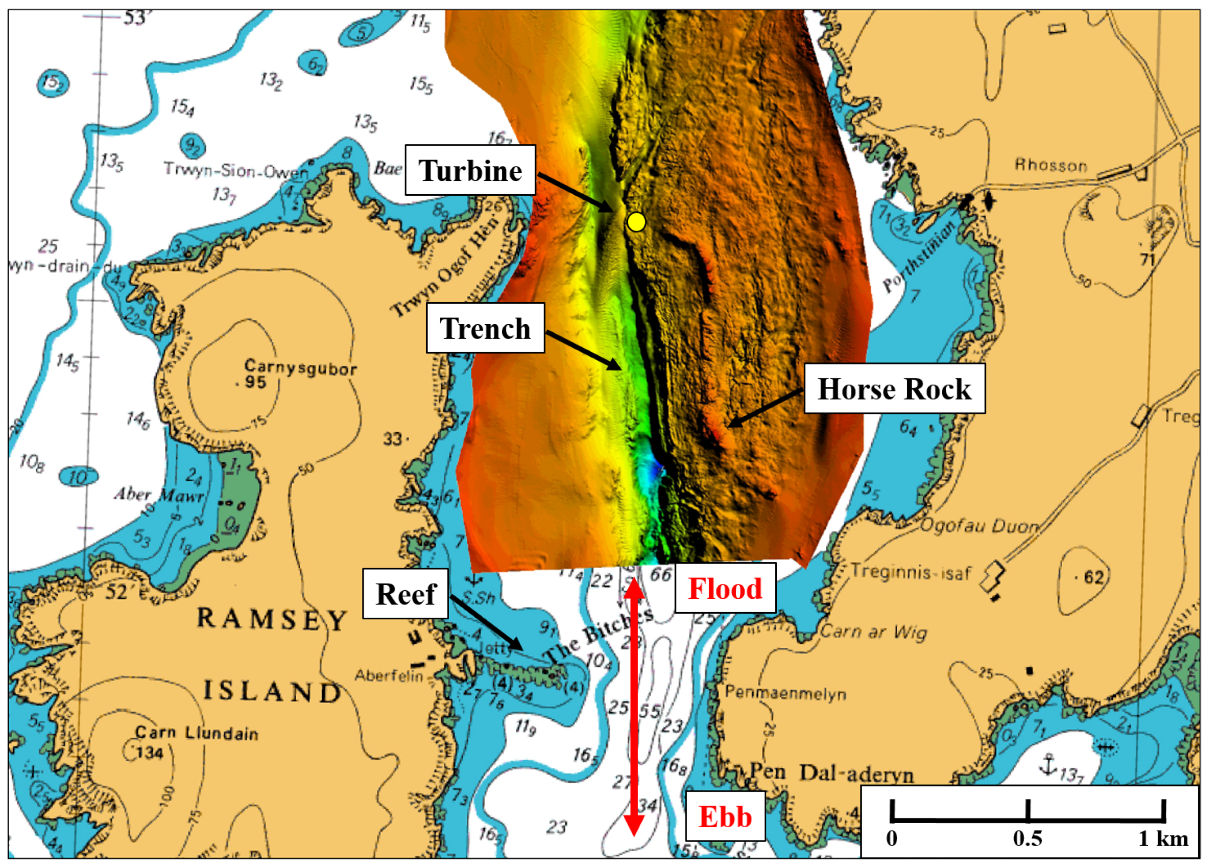
In 2015, a tidal energy company installed and grid-connected a full-scale tidal turbine in Ramsey Sound, after obtaining the required consents to develop the project. The turbine was deployed to the north of the site in a mean depth of 35 m (Figure 1), with its subsea cable travelling approximately 1.2 km eastwards to the shore at St. Justinians.

There are several notable bathymetric features that influence the hydrodynamics at the site. To the south of the turbine a trench runs through the site, with its depth reaching in excess of 75 m. East of this channel there is a long ridge that runs up towards the turbine. The ridge peaks some 700 m to the south of the turbine at Horse Rock, a large pinnacle that pierces the surface during low spring tides. Further south and outside of the extent of the bathymetric survey shown in Figure 1, a reef of rocks, known as the Bitches, protrude out into the site from Ramsey Island. In comparison, there are no significant bathymetric features to the north of the turbine and the seabed shows much less variation in depth.

2.2. Tidal Resource

As a consequence of the complex site bathymetry to the south of the turbine, the flood tides are disturbed by these seabed features and are inherently more turbulent. The flood flow is also considerably stronger at the turbine due to it being sited north of the channel narrowing that occurs at the Bitches, as well as being positioned above and north of the trench where the channel is contracted vertically. Thus, the characteristics of the ebb and flood tides at the site are not equivalent [1,8].

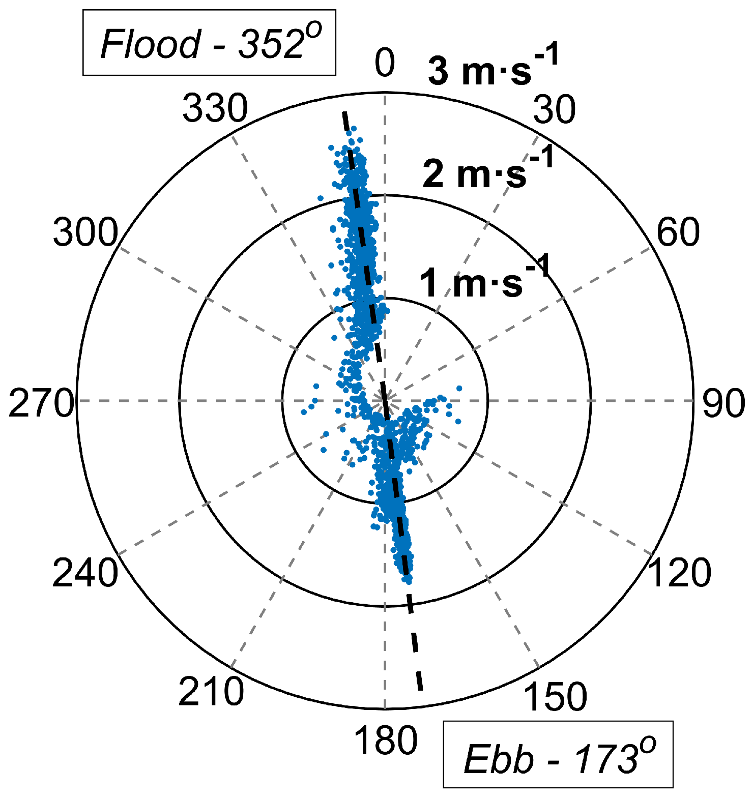
A tidal rose flow data is shown in Figure 2, obtained from a seabed mounted Acoustic Doppler Profiler (ADP) survey near the turbine location prior to its installation. The scatter, which represents 10 min average values at the turbine hub height, shows that during this survey the mean flood flow reached 2.7 m·s${}^{-1}$, whereas the maximum ebb was just 1.8 m·s${}^{-1}$. The flow is approximately bidirectional at the site, but the broader scatter seen during flood conditions highlights that the directionality is less consistent on this tide, which is a result of the bathymetry disturbing the flood flow.

3. Turbine Description

3.1. Overview

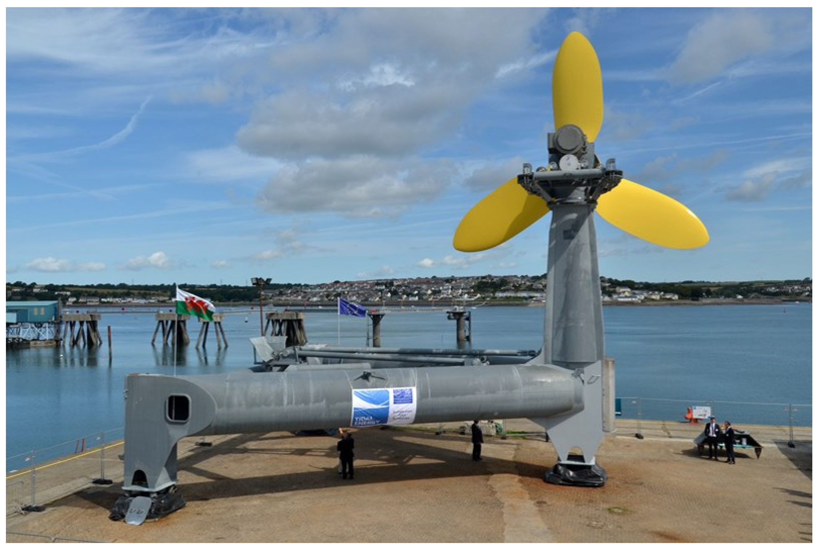
The tidal turbine installed at Ramsey Sound is shown in Figure 3. The key features of this device include: a 3-bladed, fixed-pitch rotor with a 12 m diameter; a drivetrain with a gearbox and a 400 kW induction generator; a hydraulic-based yaw system to allow the turbine to face the changing tidal current direction, or park out of the flow in non-operational conditions; and a triangular gravity-based foundation. The turbine is 18.1 m tall, meaning that its hub centre sits 12.1 m above the seabed. Power from the device was exported via a 6.6 kV subsea cable to the shore. All of the systems for power conversion and turbine control were housed onshore in a compound.

3.2. Designed Rotor Characteristics

The performance characteristics of a tidal turbine rotor are typically described using several dimensionless parameters. Firstly, the tip speed ratio, $\lambda$, is the rotor tip speed relative to the undisturbed upstream flow velocity, $U_0$:

$$\begin{array}{c}\lambda =\frac{\mathsf{\Omega }·r}{U_0}\hfill \end{array}$$

(1)

where $\mathsf{\Omega }$ and r are the rotational speed and radius of the rotor, respectively. Secondly, the rotor power coefficient, $c_p$, is the ratio of the mechanical power developed by the rotor, $P_{rotor}$, to the power available in a body of water flowing through a disk of equivalent swept area:

$$\begin{array}{c}{c}_p=\frac{P_{rotor}}{\frac{1}{2}·\rho ·\pi ·r^2·U_0^3}\hfill \end{array}$$

(2)

where $\rho$ is the water density and is typically assumed to be 1025 kg·m${}^{-3}$. Similarly, the rotor thrust coefficient, $c_t$, normalises the axial loading on the rotor, $F_{x_{\mathrm{hub}}}$, according to:

$$\begin{array}{c}{c}_t=\frac{F_{x_{\mathrm{hub}}}}{\frac{1}{2}·\rho ·\pi ·r^2·U_0^2}\hfill \end{array}$$

(3)

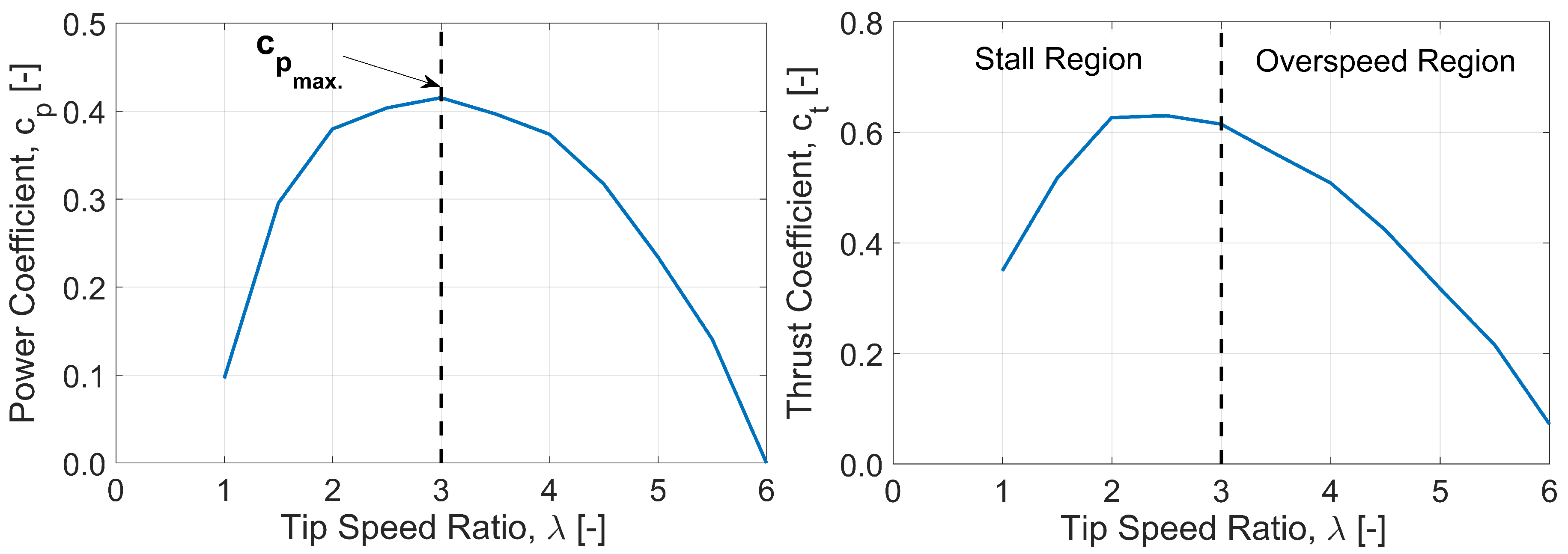
A critical design consideration for all tidal turbines is the regulation of both the developed power and mechanical loading in high flow conditions, preventing the turbine from becoming overloaded (both electrically and mechanically). Wind turbines typically achieve this through active pitch control. In this case, however, the rotor was designed such that it achieves the same objective through an overspeed control strategy, whereby the turbine is allowed to accelerate to high $\lambda$ to reduce power and axial loading. This can be seen in Figure 4, where the dimensionless characteristics of the turbine rotor are outlined from numerical model predictions, as described by Harrold et al. [16]. Prior to reaching its rated power output (400 kW), the turbine is controlled to operate at the maximum power coefficient, $c_{p_{\max .}}$, ensuring that the device maximises efficiency which is attained at $\lambda \approx 3$. Once the rated power output is achieved, the turbine caps power in higher flows by increasing $\lambda$ to a lower $c_p$, i.e., by overspeeding. This is also a region in which the $c_t$ is lower, meaning that the overspeed acts to limit both the rotor power and thrust.

The adoption of this overspeed control strategy removed the requirement for an active pitch system, ensuring that the number of sub-systems and failure modes were minimised for this first-of-kind device. Validation of the design was achieved through detailed numerical modelling [4,16] and subsequent verification from scale-model testing [17], while the overspeed philosophy has also received recent interest elsewhere [18,19]. It is worth noting that power regulation on fixed-pitch rotors is generally achieved through stall control, whereby the rotor is slowed to a lower $\lambda$. This region is also highlighted in Figure 4. However, stall control requires an increase in generator torque to slow the rotor, moving to a region of lower electrical efficiency due to increased Joule losses. The opposite is true for overspeed. Furthermore, the performance of rotors in stall is not as well understood due to several dynamic effects [20], and engineering tools are insufficient to model devices operating in this region.

3.3. Instrumentation

The turbine was equipped with a large number of sensors to monitor the condition and performance of the device, as well as its sub-systems. This work focuses on the forces acting on the turbine rotor, which were measured using fibre optic strain gauges placed on the blades. Each blade was equipped with 10 strain gauges, five on both the compression and tension surfaces and positioned at mid-chord length at rotor radial positions between 1.2–4.0 m, i.e., at distances d ranging between 0.20 $<d/R<$ 0.67. An onshore calibration was performed with the sensor manufacturer prior to the turbine installation, allowing the measured wavelengths to be converted to bending moments. The calibration also established the relevant corrections to account for thermal effects that affect the sensor readings. The sampling rate of the system was approximately 16 Hz.

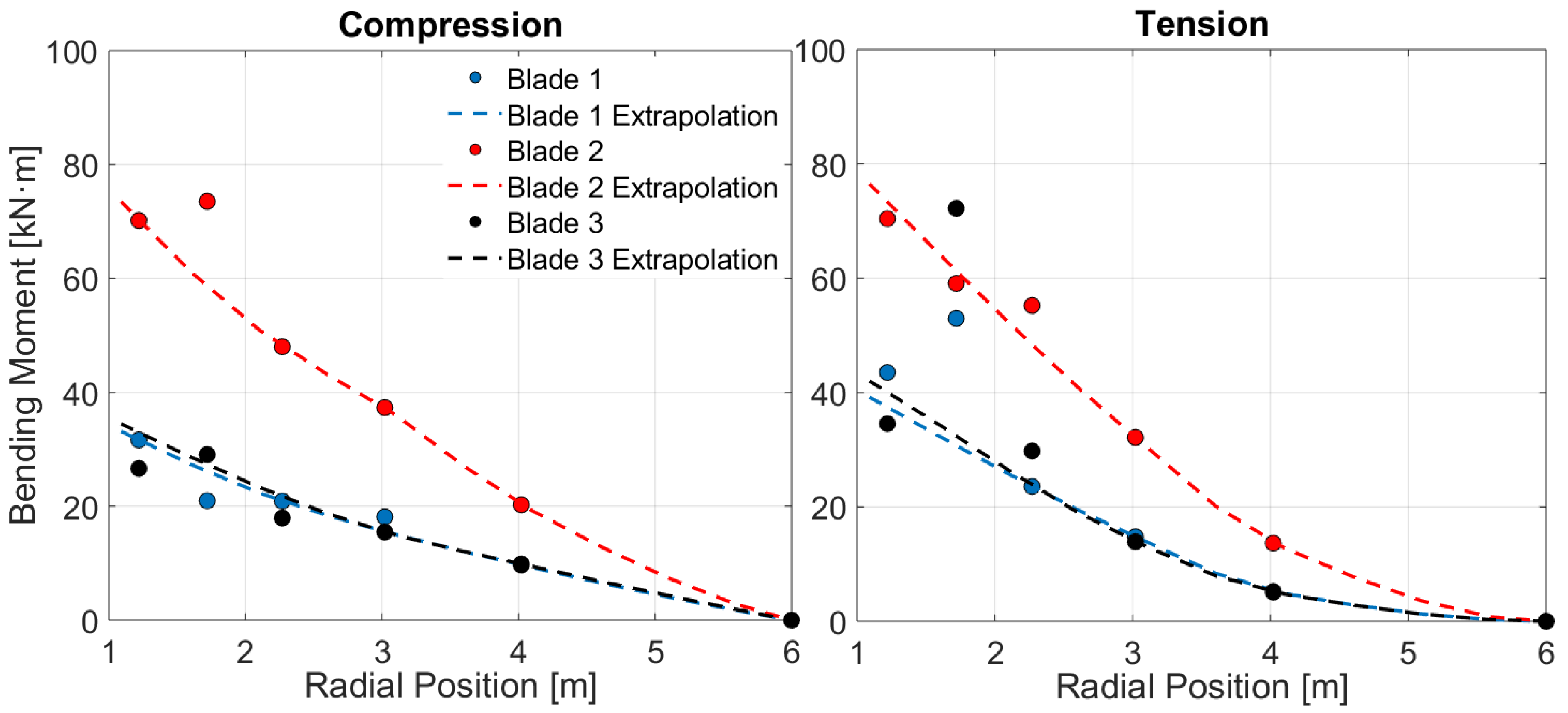
A methodology was developed to infer the blade root bending moments, $M_{y_{\mathrm{root}}}$, from the radial measurements, since the roots are subject to the highest loads and are of greater interest. The procedure involves fitting a curve to the measurements and extrapolating back to blade root radial position, which is at 1.1 m from the hub’s centre. A Matlab script was developed to perform this curve fitting procedure, using the Piecewise Cubic Hermite Interpolating Polynomial ($pchip$) extrapolation method. The methodology, however, required improvement due to some of the measurements appearing to be consistently spurious. This is thought to be a consequence of calibration difficulties at a transitional region in the blades, where the composite material changes in thickness. As a result of this, some of the radial measurements were discarded in the curve fitting process, while others had their weights modified. This increased the robustness of determining the root values, evident from improvements in the agreement of the measurements on the compression and tension surfaces of each blade, as well as the blade-to-blade measurements.

Figure 5 shows the application of this extrapolation procedure at one instance in time to the measured bending moments, both on the compression and tension surfaces of the blades. The measurements that are considerably far away from the fitted curves were discarded, e.g., at radial position 1.7 m, while those that are close to the curves have had their weights modified. A pseudo measurement was added at the blade tips, i.e., at 6 m, corresponding to the bending moment of zero experienced at these locations. This improved the curve fitting and extrapolation process. In this particular example, blade 2 was subject to the greatest amount of loading, possibly as a consequence of being orientated higher up in the water column where the tidal currents are stronger. The loading on blades 1 and 3 were comparable, suggesting they were sitting at a similar elevation. The differences of instantaneous loads between blades are constantly observed during the turbine rotation, as it is shown later in Figure 13.

Taking the derivative of the fitted bending moment profile about the root allowed the root axial forces on the blade to be determined, the summation of which yields the net rotor thrust force. The expressions for the root axial force, $F_{x_{\mathrm{root}}}$, and rotor thrust, $F_{x_{\mathrm{hub}}}$, are as follows:

$$\begin{array}{c}{F}_{x_{\mathrm{root}}}=\frac{d{M}_{y_{\mathrm{root}}}}{dr}\hfill \end{array}$$

(4)

$$\begin{array}{c}{F}_{x_{\mathrm{hub}}}=\sum F_{x_{\mathrm{root}}}\hfill \end{array}$$

(5)

The root loads and rotor thrust were calculated independently using the compression and tension strain gauges, providing two measurements of each. For the analysis that follows, the reported loads are the mean of these two measurements.

This procedure for calculating thrust differs from that typically used in scale-model studies [17] or field testing of smaller rotors [12], where load cells are placed on the turbine support structure and a correction is applied to remove the drag forces acting on the structural elements, leaving only the axial force on the rotor. This involves measuring the drag on the support structure without the rotor, something that was not practical for the turbine in this study and would not provide any information on the individual blade loading and bending moments.

In addition to the turbine sensors, several environmental sensors were used to determine the effects of the environment on the turbine and vice versa. This included two ADPs to measure the local flow velocities, hereafter referred to as the seabed and turbine ADPs. The seabed ADP is a 600 kHz Teledyne RDI Workhorse Sentinel 4-beam instrument, which was placed in a small gravity frame 35 m eastwards of the turbine. This instrument was configured to sample at 1 Hz with a 0.75 m bin resolution, providing information on the vertical tidal current profile and directionality. However, the instrument does not necessarily provide a good reference of the tidal currents experienced by the turbine due to the significant lateral distance between the two, which might be subject to horizontal shear. The IEC 62600-200 guidelines on tidal turbine power performance assessment recommend that ADPs are placed between 1–2 equivalent rotor diameters away from the rotor plane extent in this configuration (orientation B) [21], which in this case would be between 18–30 m away from the rotor centre. Furthermore, these guidelines recommend that two ADPs are placed either side of the turbine in this configuration, with the velocities averaged between the ADPs to evaluate the flow experienced by the turbine. Since these conditions could not be met, the seabed ADP was not considered a suitable reference for the turbine characteristics herein presented. Instead, it is a useful additional measure of the ambient flow conditions at the site.

The turbine ADP is a 1 MHz Nortek Aquadopp instrument, fitted with a bespoke single-beam head piece. The instrument was placed inside the turbine nosecone to profile the line-of-sight currents approaching the rotor, sampling at 1 Hz with a 1 m bin resolution to a range of 20.4 m upstream, i.e., 1.7 rotor diameters. The IEC 62600-200 currently does not recognise this instrument configuration for assessing the power performance of tidal turbines, despite several device developers adopting it. The benefits include: just one ADP is required provided that the turbine has yaw capability; there is no requirement for additional marine installations of seabed structures to house ADPs; the instrument can be powered from shore along with the other turbine systems, preventing any limitations on battery life and data storage; and the instrument always measures the incident rotor flow, reducing uncertainty related to misalignment. Since the seabed mounted ADP cannot be considered an appropriate upstream reference of the velocity experienced by the rotor, the turbine ADP is used for this purpose in the following sections.

4. Results and Discussion

4.1. Site Layout and Characterisation

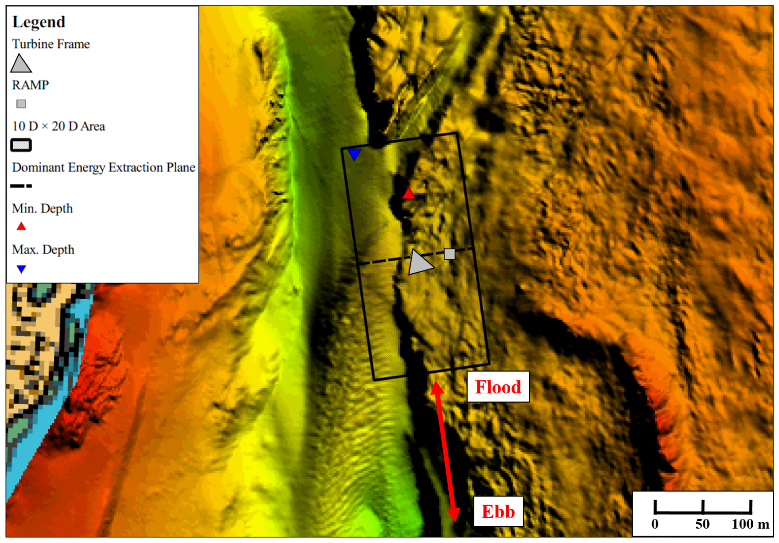
To assess whether there are any features of the seabed that could affect device performance, industry guidelines [21] recommend surveying the bathymetry at the deployment site out to 5 equivalent rotor diameters (D) either side of the turbine, and 10 D upstream and downstream, covering an area of 10 D × 20 D. This region is shown in Figure 6, with the area offset by 8${}^{\circ }$ to align with the dominant flow directions (see Figure 2). The turbine sits on the northernmost apex of its triangular frame with the rotor facing west when parked and non-operational. The yaw system range (±100${}^{\circ }$) was sufficient to allow the rotor to face the dominant directions of both tides, and accounted for the small offset frame installation angle from true north. The seabed ADP was housed in a small structure referred to as the Remote Acoustic Monitoring Platform (RAMP), and was cabled to the turbine in order to receive power from the shore and to enable live data transfer.

The turbine sits on a relatively flat ridge to the east of the northern portion of the trench that runs through Ramsey Sound. The depth extremities within the 10 D × 20 D area range from 31 m at just over 5 D to the north of the turbine, to 44 m near the north-west apex of this considered area. Compared with the seabed features found elsewhere in Ramsey Sound (see Figure 1), this local depth variation is not considered significant. Both the RAMP and turbine sit at a mean depth of 35 m.

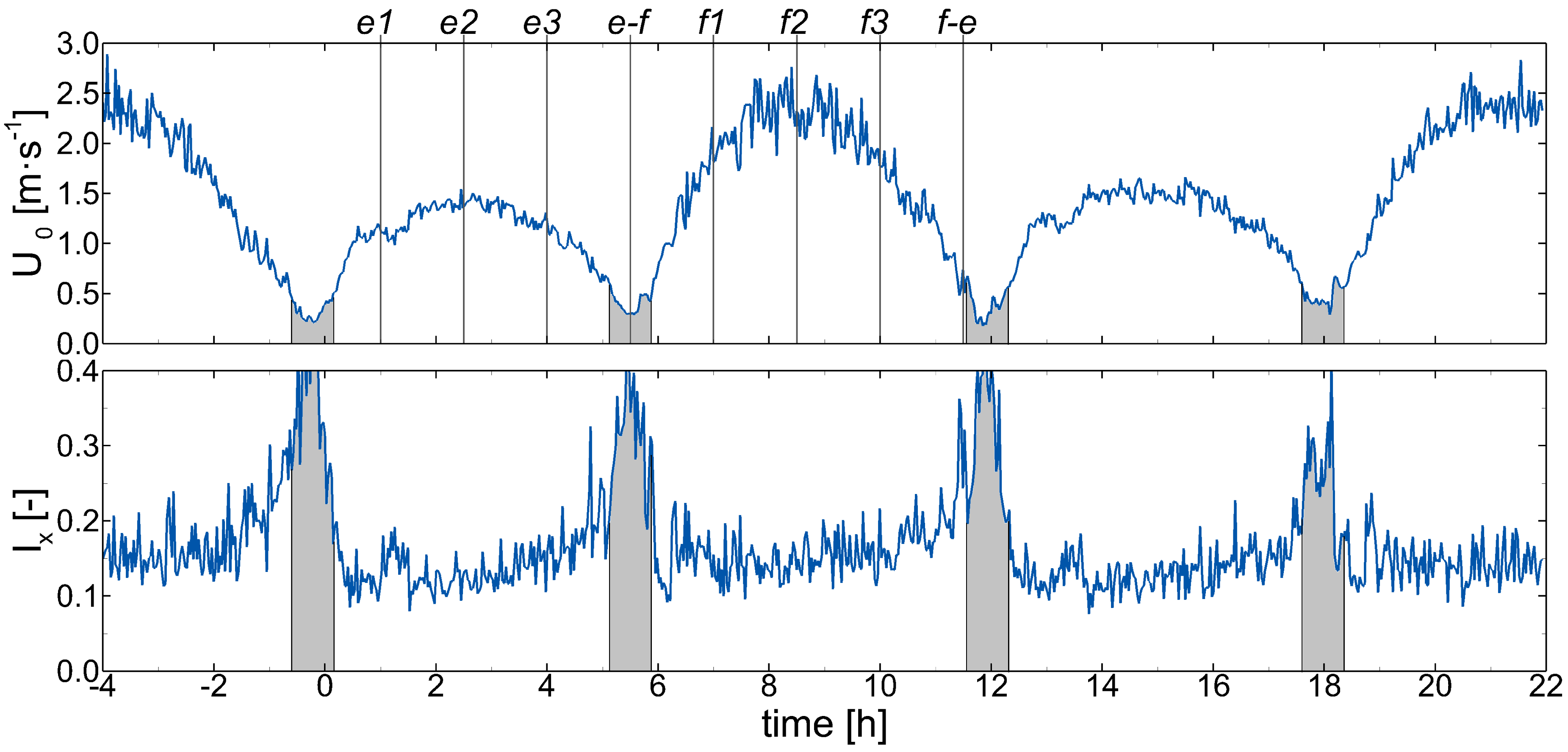
The flow characteristics of two full tidal cycles at the site are presented in Figure 7, measured with the seabed mounted ADP using the hub height bin only (z = 12.1 m), i.e., at a relative submergence of $z/H$ = 0.35. The measurements are of 10 min time-averaged velocity ($U_0$) and turbulence intensity ($I_x={\sigma }_{u_i}/U_{0_i}$, with $U_{0_i}$ denoting mean velocity and ${\sigma }_{u_i}$ is the root-mean-square of the velocity fluctuations during the i-th bin). Shaded grey areas in Figure 7 outline periods of slack water with flow velocities below a velocity threshold of 0.5 m·s${}^{-1}$. There was an important variation of velocities between tidal phases evidencing the asymmetric flow pattern at the site. During flood tides, the flow was characterised by large velocities reaching values over 2.5 m·s${}^{-1}$, while ebb tides attained peak velocities up to 1.45 m·s${}^{-1}$. During slack water periods, turbulence levels greatly increased with values over $I_u=$ 0.4, but these did not challenge the structural integrity of the turbine as the flow velocities were low and the device did not operate under such conditions.

Approach flow velocities across the measured water column during both ebb and flood tidal phases exhibited a time-dependent pattern, both in its vertical distribution and magnitude. This behaviour is observed in Figure 8 which presents the values of $U_0$ and $I_x$ measured with the seabed ADP at depths between 3.1 m $<z<$ 30.1 m at eight different time intervals, covering both ebb and flood tides depicted in Figure 7. At the onset of the turbine operation during ebb tide, i.e., at $\mathit{e}1$, the flow overcame 1 m·s${}^{-1}$ velocity, and ebb tide peak velocities of approximately 1.5 m·s${}^{-1}$ were reached at $\mathit{e}2$. The velocity distribution at the falling ebb tide, specifically at $\mathit{e}3$, attained a very similar distribution to that at $\mathit{e}1$, although with a slight difference found below hub height.

Figure 8b shows that during the flood phase, velocities in the rising flood profile ($\mathit{f}1$) seem to follow a logarithmic distribution until hub height, but higher up in the water column the velocities do not increase much and are nearly constant at a value of 2 m·s${}^{-1}$. At peak flood tide, i.e., $\mathit{f}2$, the maximum velocities were observed at elevations higher than the hub height with a larger region of the water column following a logarithmic distribution than at $\mathit{f}1$. In the transition from flood flow to slack water, at $\mathit{f}3$, the vertical distribution of velocities was very similar to $\mathit{f}1$, although with a lower maximum value of 1.7 m·s${}^{-1}$. From Figure 8a,b it can be observed that the velocity distributions during ebb flow can be approximated to a logarithmic profile, whereas in the flood tide the velocities do not always follow such behaviour over the entire water depth, as found by others [2,8].

Turbulence intensity profiles, shown in Figure 8c,d, depict again the notably asymmetric flow conditions during ebb and flood tides and variability within each tidal phase. At peak ebb flow, maximum values of $I_x$ were found near the seabed and free-surface, attributed to bathymetry-induced and wave effects respectively, and minimum values were attained just above the turbine top tip, i.e., $z\approx$ 20–22 m. Conversely, during flood tide the lowest turbulence intensity levels were found close to the hub height whereas maximum values were again observed near the lowest and highest locations in the water column.

The variation in the spatial characteristics of turbulence suggests that the turbine’s blades face anisotropic turbulent flow conditions during its operation. The time-dependent heterogeneous distribution of $I_x$ between ebb and flood tides was also found at other sites such as the Sound of Islay (UK) where the turbulence intensities can vary between 0.11 and 0.13 during flood and ebb tides respectively, or at the East river (US), which is slightly more turbulent attaining values of $I_x$ equal to 0.13 (flood) and 0.18 (ebb) [22].

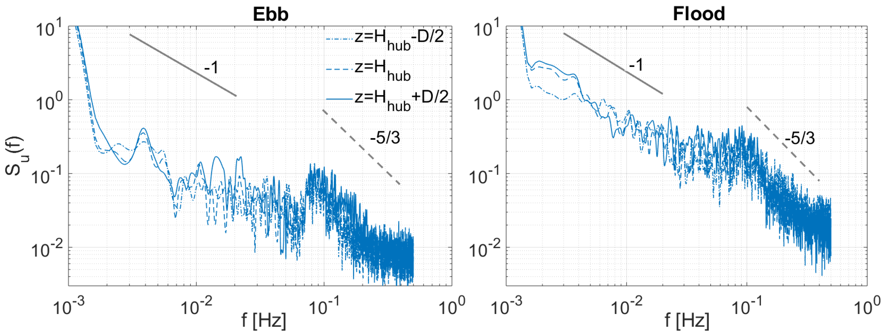
Further analysis of the spatial variability of the velocities across the water column is performed in Figure 9 with the Power Spectral Density (PSD) distribution of 10 min bin velocities during peak flood and ebb tides at hub height ($H_{hub}$) and at bottom and top tips, i.e., $z=H_{hub}\pm D/2$. The $pwelch$ function was used to compute the spectra, dividing the signal into 20 ensembles. The spectra suggest that energy decay during the production range followed a −1 slope commonly found in boundary-layer flows [23,24], and the spectral energy ($S_u$) associated with the lowest frequencies was greater during flood tide, indicating that the largest flow scales approaching the turbine during this phase were more energetic than during ebb. This is expected as the flow velocities during flood were greater than in ebb (see Figure 8).

The spectrum at z = $H_{hub}-D/2$ during flood tide presents a lower spectral energy than those computed at higher elevations, identifying the spatial variation of the flow dynamics within the turbine’s swept area. Such flow variability at the deployment site, due to the irregular bottom bed shape (Figure 6) among other local features, are well-identified from both the vertical profiles of time-averaged velocity statistics and power spectral energy distribution, shown in Figure 8 and Figure 9 respectively. Previous studies acknowledging the tidal flow asymmetry of Ramsey Sound were reported in [1,8,25].

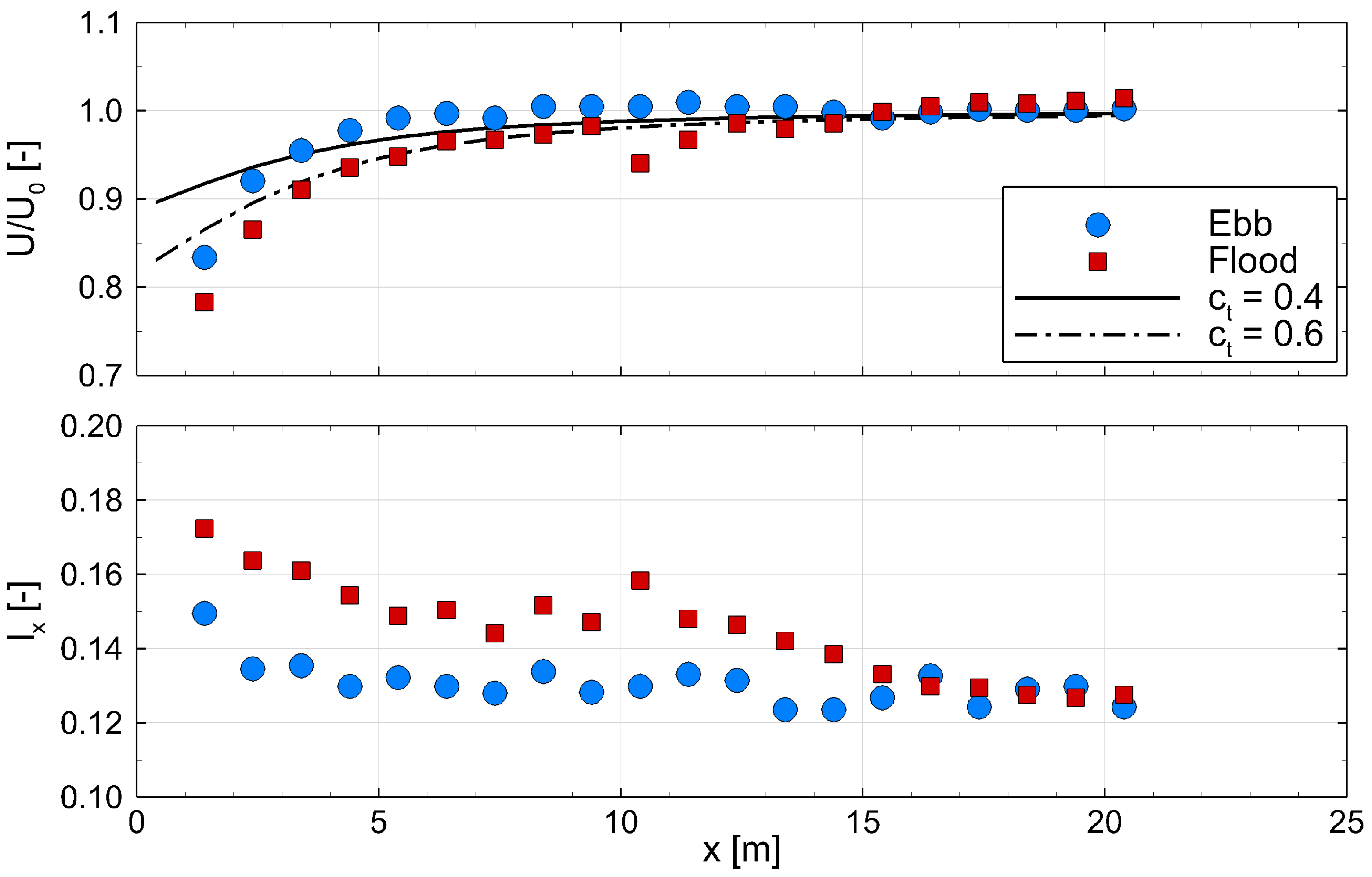
Distribution of flow velocities upstream of the turbine in the range between 1.4 m to 20.4 m measured with the turbine ADP are shown in Figure 10, with the mean velocities and turbulence intensities calculated over 10 min bins during peak ebb and flood, i.e., e2 and f2. The inflow velocities are normalised by the mean of the values obtained at an upstream range, x, greater than one rotor diameter (12 m), which are the outermost eight ADP bins. This definition is considered the undisturbed free-stream velocity, $U_0$, since the measurements from this range are generally within 2% of each other. The velocities were subject to a considerable reduction near the rotor due to the flow moving around the turbine. This behaviour has been observed by others using a similar turbine mounted ADP arrangement [26].

Furthermore, velocity measurements in Figure 10 are compared with vortex sheet theory [27] based on different thrust coefficients of the turbine, represented in terms of the induction factor (a), which determines the upstream velocity as:

$$\begin{array}{cc}\hfill a& =\frac{1}{2}\left(1-\sqrt{1-c_t}\right)\hfill \end{array}$$

(6)

$$\begin{array}{cc}\hfill \frac{U}{U_0}& =1-a\left(1+\frac{2x}{D}{\left(1+{\left(\frac{2x}{D}\right)}^2\right)}^{-1/2}\right)\hfill \end{array}$$

(7)

A reasonable agreement is found between field velocities and vortex sheet theory during both tidal phases at upstream distances of $x>$ 6 m irrespective of the thrust coefficient attained by the turbine, which signifies Equation (7) can be used to approximate the tidal flow velocities that approach the turbine, analogous to those obtained in wind turbine research [27,28]. The reduction on the approach velocity was consistently found to be greater during flood tides, believed to be a consequence of the flow being disturbed by the triangular frame supporting the turbine (Figure 3), which contributes to a larger flow deceleration at $x<$ 5 m than that predicted by the vortex sheet theory. The frame only sits upstream of the rotor during flood tides (Figure 6), with its front edge approximately 10 m upstream of the rotor. This was consistent with the location of a small trough in the approaching flood velocity and a peak in turbulence intensity.

The turbulence intensity near the rotor was also found to be consistently higher during flood, whereas further upstream (x > 15 m) the levels are not dissimilar to ebb (12–14%). These features were observed throughout the flood measurements, and provide further evidence of the turbine frame disturbing the approaching flow. Since these observations have been made on the turbine ADP which sat at an elevation of almost 8 m above the frame height, it should be expected that the flow disturbances were greater at lower elevations, i.e., in the lowermost regions of the blade rotations.

4.2. Turbine Operation

To measure the non-dimensional rotor characteristics, the turbine was operated in a speed controlled mode such that its objective was to hold a fixed rotational speed, Ω. The turbine controller would in response vary the generator torque in order to maintain the commanded rotor speed, regardless of the flow conditions. This mode was used to step the rotor through various rotational speeds during both ebb and flood tides. Provided that each step change was not accompanied by a proportional change in mean flow speed, the turbine would operate at a different tip speed ratio. This procedure is akin to methodologies adopted in scale-model test studies of tidal turbines [17,29].

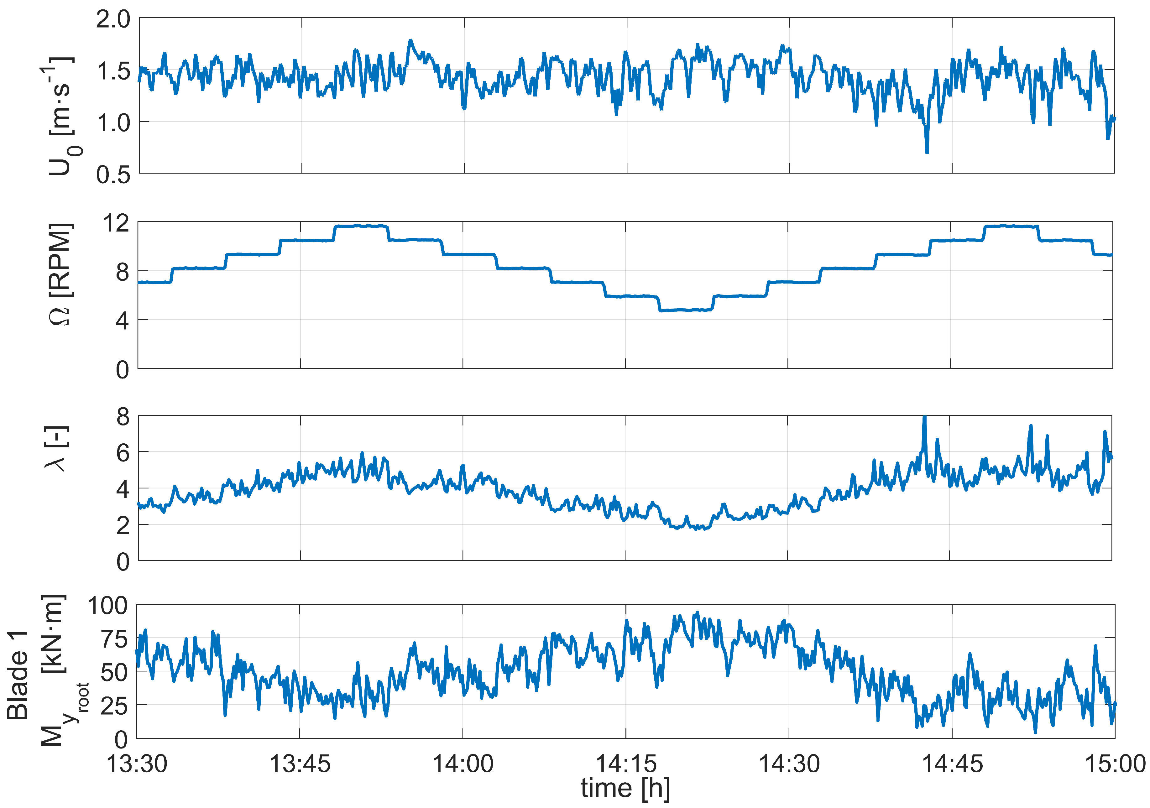
Figure 11 shows the time-series of approach flow velocity ($U_0$), turbine rotational speed ($\mathsf{\Omega }$), tip speed ratio ($\lambda$), and blade root bending moment ($M_{y_{\mathrm{root}}}$) from a test that took place during an ebb tide, with all values representing 10 s averages. The upstream flow velocity here were measured from the turbine ADP and as defined in Section 4.1. The rotor speed was stepped within the range 5–12. Revolutions Per Minute (RPM), leading to a tip speed ratio generally between 2–5. There was a clear trend of decreasing blade root bending moment with increasing tip speed ratio, i.e., maximum bending moments in the range of 80 kN·m were attained at $\lambda \approx 3.0$, while these reduced to 35 kN·m when $\lambda \approx 5.0$, demonstrating the overspeed load reduction characteristics of the rotor, as shown in Figure 4. During the 1.5 h time period presented in Figure 11, the approach flow appeared to be turbulent with high-frequency velocity changes causing the turbine loadings to vary remarkably even within the same step period, which provides evidence of the complexity of testing full-scale devices in real-sea conditions.

One potential drawback of this test procedure is that the tip speed ratio was not fixed during the stepping periods, only the rotor speed was. It is possible that this could lead to a bias in the calculation of rotor coefficients. Better control of the tip speed ratio could have been achieved by changing the gain applied to the generator torque in a variable speed turbine control scheme, but this functionality was not possible at the time of testing. However, the results from previous testing of this rotor at model scale using the same RPM stepping method proved to very repeatable [17].

4.3. Hydrodynamic Loading Coefficients

In addition to the rotor thrust coefficient (Equation (3)), the following dimensionless parameters are used to describe the blade root bending moments, $c_{M_{y_{\mathrm{root}}}}$, and axial forces, $c_{F_{x_{\mathrm{root}}}}:$

$$\begin{array}{c}{c}_{M_{y_{\mathrm{root}}}}=\frac{M_{y_{\mathrm{root}}}}{\frac{1}{2}·\rho ·\pi ·r^3·U_0^2}\hfill \end{array}$$

(8)

$$\begin{array}{c}\hfill \\ c_{F_{x_{\mathrm{root}}}}=\frac{F_{x_{\mathrm{root}}}}{\frac{1}{2}·\rho ·\pi ·r^2·U_0^2}\hfill \end{array}$$

(9)

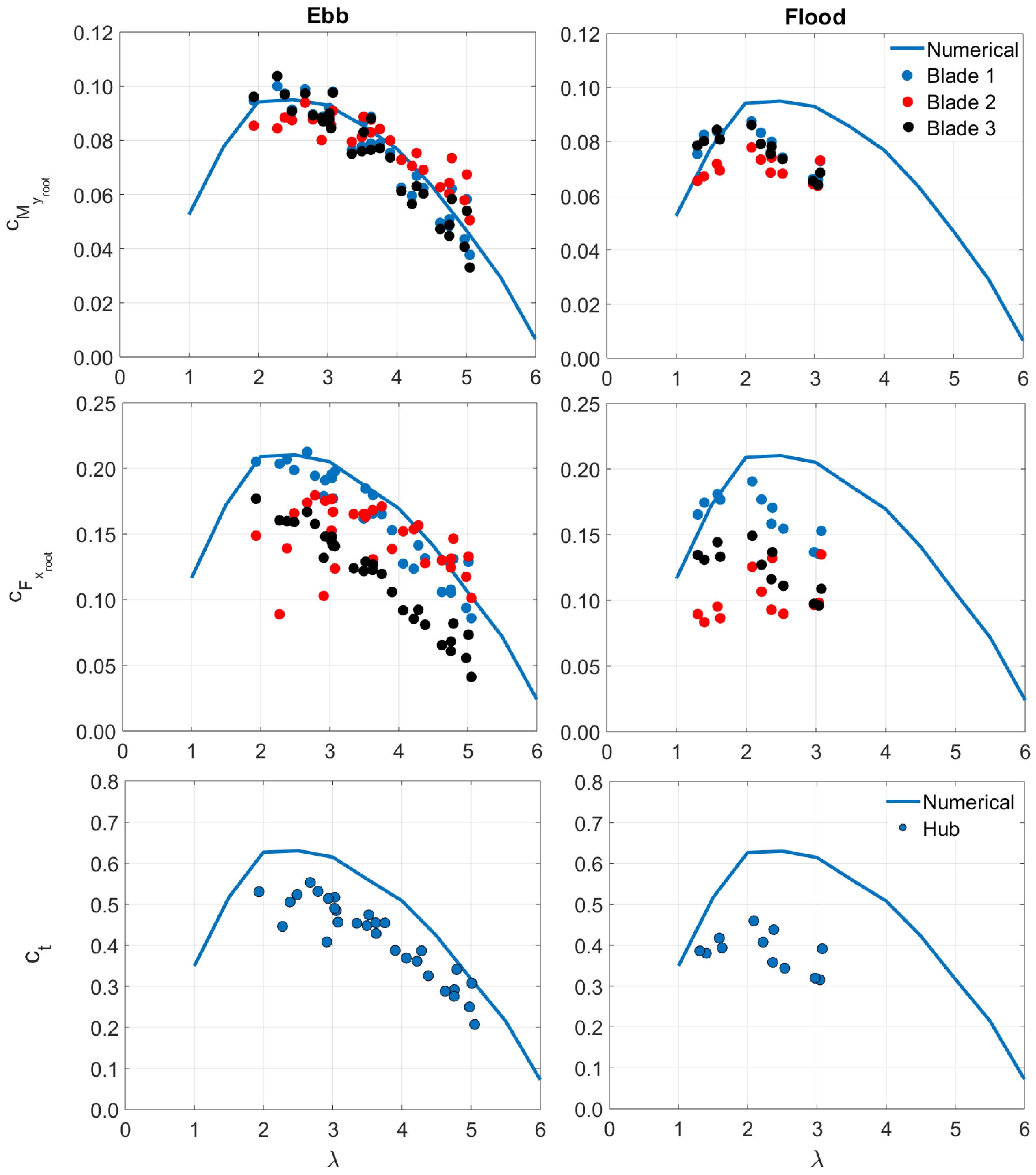
Dimensionless rotor loading characteristics measured during ebb and flood tides are presented in Figure 12, compared with numerically predicted curves from a Blade Element Momentum-based model described in Harrold et al. [16]. These simulations were performed under steady conditions, with the turbine running at a fixed speed in a uniform flow field. The measurements represent the mean values from within the rotor speed stepping periods after discarding measurements from within 10 s of each step change in order to allow some settling time.

Considering firstly the results obtained during ebb conditions, the measured $c_{M_{y_{\mathrm{root}}}}$ values show a very good agreement with the theoretical prediction for each of the three blades, scattering closely about the numerical curve. Similarly, the measured $c_{F_{x_{\mathrm{root}}}}$ values on blade 1 are in good agreement with the theoretical curve and the predicted trend of decreasing $c_{F_{x_{\mathrm{root}}}}$ with increasing $\lambda$ is clear in the results from all of the blades. However, the measured $c_{F_{x_{\mathrm{root}}}}$ values show greater blade-to-blade variation and their magnitudes are generally lower than the theoretical prediction. This can be attributed to the derivation of $F_{x_{\mathrm{root}}}$ as described in Section 3.3, in which this load was entirely dependent on the shape of the curve fitted to the measured radial bending moments. While some aforementioned measures were introduced to improve the robustness of this process, it is clear that further refinement is required to improve the derivation of $F_{x_{\mathrm{root}}}$, particularly on blades 2 and 3. In contrast to this, the derivation of the $M_{y_{\mathrm{root}}}$ values only required a simple extrapolation and, as a result, a better agreement was found, both in terms of the blade-to-blade results and with the numerical model prediction. The difficulties encountered with the $F_{x_{\mathrm{root}}}$ measurements also led to lower than expected rotor thrust loading, although the shape of the $c_t$ curve was captured well.

To improve the measurements of the rotor loads, ideally a secondary calibration and the relocation of the problematic sensors on the blades at radial position 1.7 m would have been performed, but this would have required the physical removal of the turbine from the site. The existing procedure could be improved by further modification of the applied weighting to measurements, such that the agreement between $F_{x_{\mathrm{root}}}$ loads calculated on the compression and tension surfaces of the blades improves. Similarly, any modifications should attempt to improve the agreement between blade-to-blade $F_{x_{\mathrm{root}}}$ averaged over a long enough period, i.e., a sufficient time interval to reduce any bias being introduced from the loads changing on the blades during rotation.

As for the flood tide results, fewer measurements were obtained during these conditions and only within the tip speed ratio range 1–3, limiting the data available to compare with those obtained in ebb. However, in the region that does overlap with the ebb measurements, i.e., between $\lambda$ = 2–3, the mean loads were consistently lower in flood conditions. For example, the $c_{M_{y_{\mathrm{root}}}}$ measurements mostly cluster around a value of 0.065 at $\lambda$ = 3 during flood, whereas in ebb they were found at values close to 0.087. It is believed that this is directly attributable to the reduced inflow and increased turbulence found during flood conditions, as observed in Figure 10. Since the loading coefficients and $\lambda$ were calculated relative to the undisturbed upstream flow at hub height, the reduced inflow observed near the rotor during flood was not accounted for, nor was the slowing of velocities higher up in the water column (Figure 8). Therefore, a reduction in mean rotor loading was experienced during flood due to the influence that the turbine frame structure and site bathymetry have on the inflow.

4.4. Instantaneous Structural Loadings

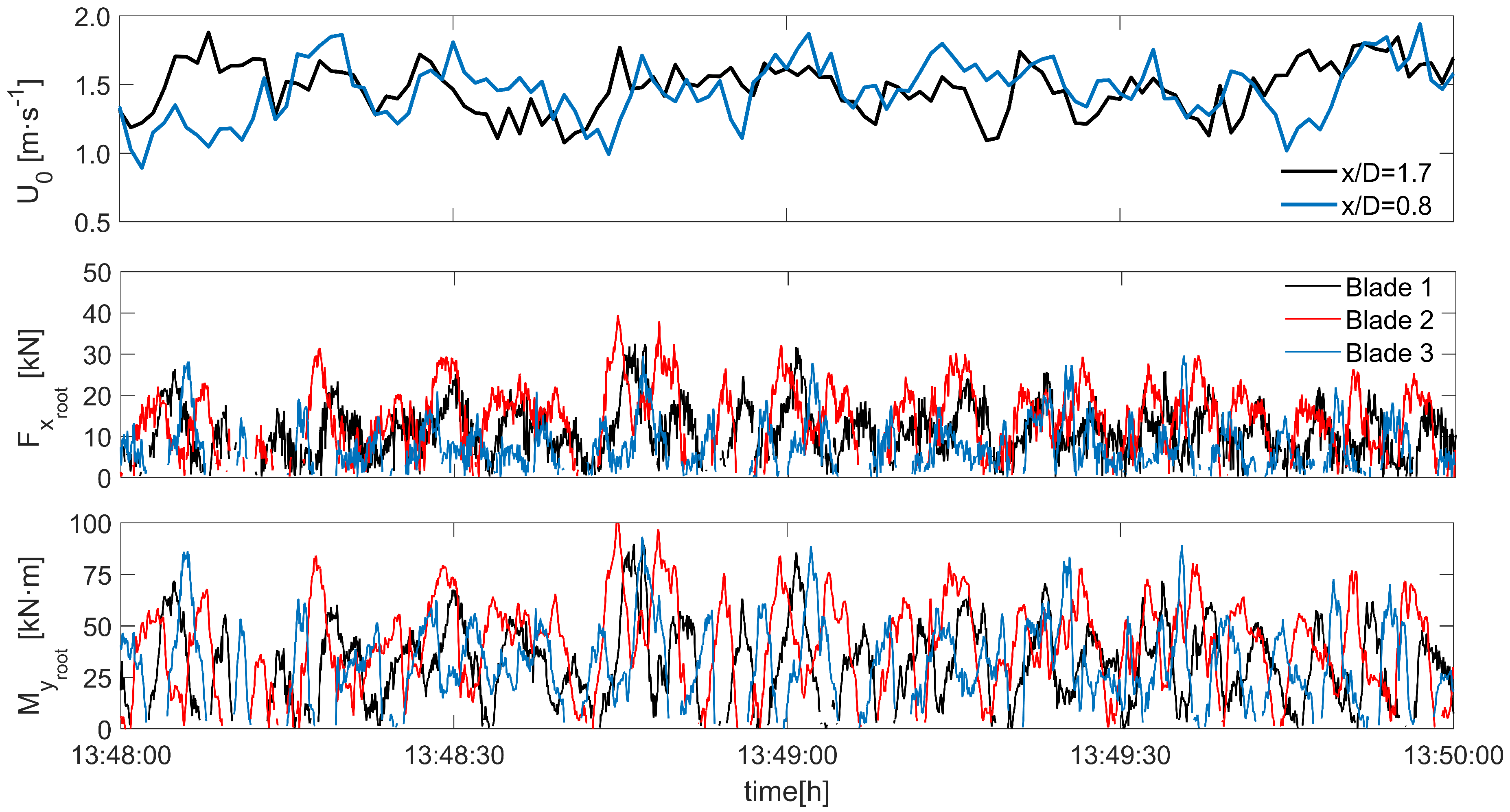
Instantaneous variation of structural loadings as a result of the fluctuating approach velocity is presented in Figure 13 with velocities measured with the turbine ADP from bins located at distances x = 9.4 m and 20.4 m, i.e., 0.8 D and 1.7 D, upstream of the turbine, and measurements of axial force and bending moment at the root of the three blades. These data correspond to a 2-min snapshot of the 5-min stepping period in which the turbine operated at a fixed rotational speed of $\mathsf{\Omega }$ = 11.61 RPM during the ebb tide presented in Figure 11. Velocity measurements at two different distances from the turbine are presented to observe the local flow variation within the short distance of 11 m before impinging the turbine. All the blades undergo similar magnitudes of structural loadings, although the peaks at the same rotation interval did not attain the same value, i.e., blades experienced different extreme loads during their operation as the flow is markedly uneven across the rotor swept area. Similar results of uneven load distributions among blades were found in Ouro and Stoesser [24] who performed high-fidelity simulations of a turbine operating over irregular bathymetry.

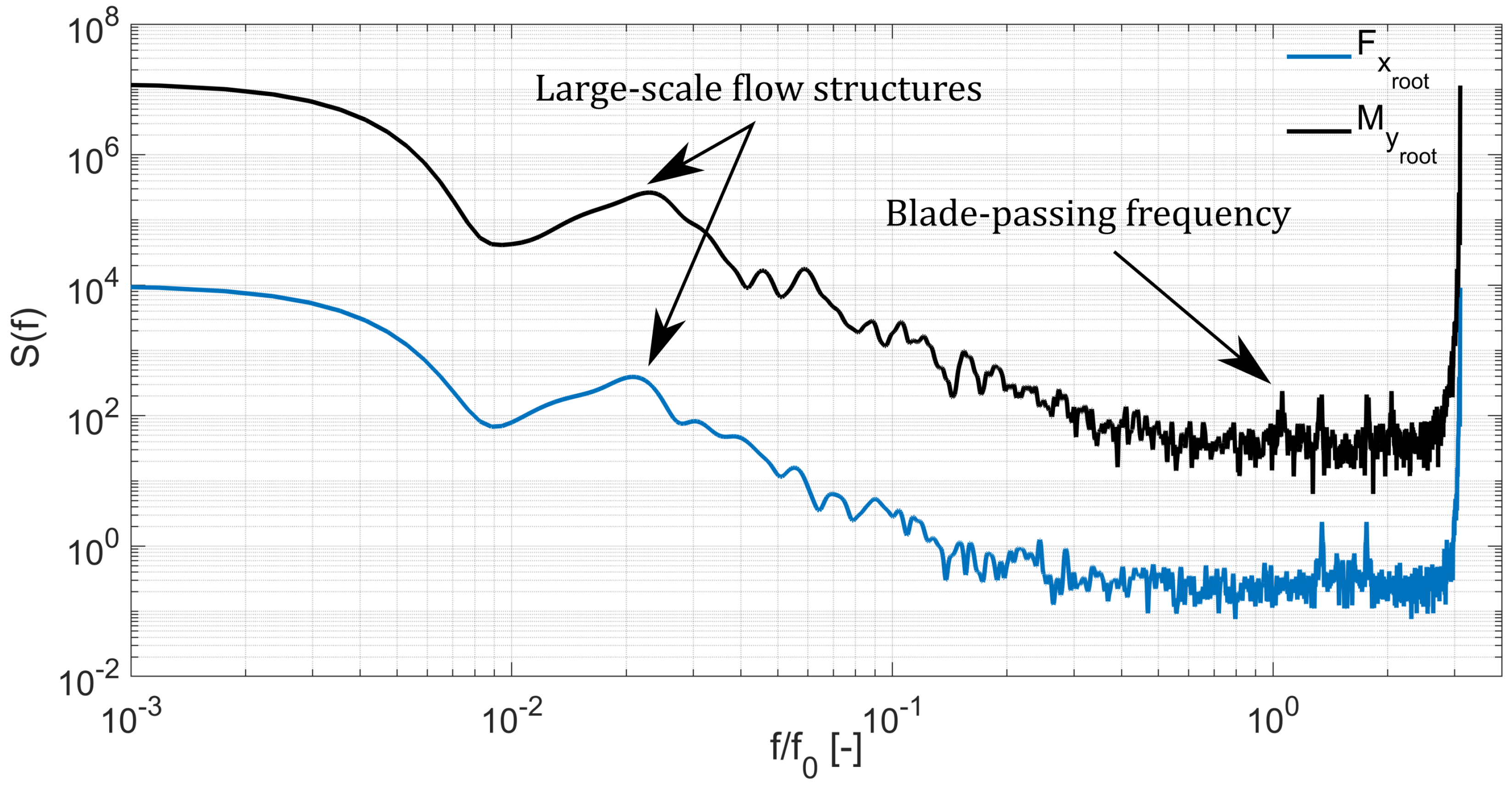
The distribution of spectral energy of $F_{x_{\mathrm{root}}}$ and $M_{y_{\mathrm{root}}}$ across relevant frequencies is presented in Figure 14, with the spectra computed from the loadings on one of the blades during the 5 min interval shown in Figure 13, applying an analogous procedure as for the velocity spectra from Figure 9. Frequencies are normalised by the turbine rotational frequency $f_0$ = $(\mathsf{\Omega }$(RPM)/60 s) $\approx 0.193$ Hz. At frequencies in the range of $f/f_0\approx 2\times {10}^{-2}$ there is a peak in spectral energy in both axial load and bending moment associated with low-frequency velocity oscillations resulting from the action of large-scale flow structures. Note that this frequency coincides with the transition from the production range to the inertial sub-range obtained from the velocity spectra in Figure 9.

An energy peak is observed at a frequency of $f_0$ derived from the periodic change in the blade loadings during every rotation, which is only observed in the bending moment spectrum. The spectral energy linked at a frequency of $f_0$ has a similar magnitude to peaks found at higher frequencies, despite previous data from laboratory tests showing that the maximum energy may be attained at the the turbine rotational frequency [11]. These results can be linked to the relatively short sampling period of 5 min and due to high turbulent flow conditions in which the full-scale device operated unlike the fairly controlled conditions that are normally found during laboratory testing. Two peaks in the $F_{x_{\mathrm{root}}}$ and $M_{y_{\mathrm{root}}}$ spectra are found at frequencies of 1.35 $f_0$ and 1.70 $f_0$ owed to blade-rotation effects, and only in the latter spectrum another peak is observed at 2.0 $f_0$. Finally, a large energy peak whose frequency is almost that of the data acquisition and harmonic of the rotation frequency, i.e., 16 Hz, is clearly observed from the spectra. Similar spectral energy distribution of the loadings on a prototype turbine in the frequency domain were found in Payne et al. [11] who also discerned that peaks can vanish when the turbulence intensity in the approach flow is high.

5. Conclusions

This study reports on the operational measurements from a full-scale tidal stream turbine. The turbine was deployed at Ramsey Sound (Wales, United Kingdom), which is characterised by a highly irregular bathymetry that leads to significant flow unsteadiness and variation during ebb and flood tidal phases. A methodology was devised to infer the forces acting on the turbine rotor from strain gauges placed in the blades. The study related these measurements to those of the ambient flow conditions in order to assess how the loading on the turbine was influenced by turbulence in the tidal currents.

Following a similar methodology to scale-model test studies, the structural behaviour of the turbine was analysed using a stepping method in which its rotational speed was fixed during 5 min intervals. The blade root bending moments were found to decrease at high tip speed ratios, i.e., when the turbine was overspeeding, and were also lower than those measured in the stall region. These results demonstrate the potential of an overspeed-based control strategy in mitigating excessive loading on the turbine, which can be achieved without the requirement of a pitch system to feather the blades.

The mean dimensionless hydrodynamic coefficients of the blade and rotor loads were derived during this test, covering the tip speed ratio range $\lambda$ = 2–5 in ebb conditions and $\lambda$ = 2–3 in flood. The observations during ebb agreed well with Blade Element Momentum-based numerical predictions of the rotor loading, particularly the blade root bending moment coefficients. However, the flood measurements were found to be considerably lower than the theoretical predictions due to the disturbance of the approach flow from a combination of the turbine frame structure and the uneven site bathymetry upstream of the device during this tide. It is worth noting there was also an appreciable amount of scatter in blade-to-blade results for the measured axial root forces, leading to lower than expected rotor thrust. Further calibration is required in the methodology used to derive these loads in order to increase the reliability of results. Despite this, the measurements of the blade root bending moments were found to be much more consistent, owing to the fact that only a simple extrapolation was required in their derivation. These results, therefore, can be relied upon to support the key findings.

Instantaneous variations of the loadings at low and high frequencies were observed signifying that the approach flow was characterised by a wide spectrum of scales. At some rotations, different peak values were observed for each blade as a consequence of them being impacted unevenly by these energetic flow structures. Spectral analysis of the loadings confirmed the relevance of the largest flow scales in their low-frequency change in addition to those induced from the turbine rotation. Overall, this study also provides evidence for the complexity experienced when testing full-scale turbines at sea due to the uncontrolled environment leading to increased flow and measurement uncertainties.

References

- Evans, P.; Mason-Jones, A.; Wilson, C.; Wooldridge, C.; O’Doherty, T.; O’Doherty, D. Constraints on extractable power from energetic tidal straits. Renew. Energy 2015, 81, 707–722. [Google Scholar] [CrossRef]
- Lewis, M.; Neill, S.; Robins, P.; Hashemi, M.; Ward, S. Characteristics of the velocity profile at tidal-stream energy sites. Renew. Energy 2017, 114, 258–272. [Google Scholar] [CrossRef]
- Mycek, P.; Gaurier, B.; Germain, G.; Pinon, G.; Rivoalen, E. Experimental study of the turbulence intensity effects on marine current turbines behaviour. Part I: One single turbine. Renew. Energy 2014, 66, 729–746. [Google Scholar] [CrossRef]
- Ouro, P.; Harrold, M.; Stoesser, T.; Bromley, P. Hydrodynamic loadings on a horizontal axis tidal turbine prototype. J. Fluids Struct. 2017, 71, 78–95. [Google Scholar] [CrossRef] [Green Version]
- Blackmore, T.; Myers, L.; Bahaj, A. Effects of turbulence on tidal turbines: Implications to performance, blade loads, and condition monitoring. Int. J. Mar. Energy 2016, 14, 1–26. [Google Scholar] [CrossRef] [Green Version]
- Milne, I.; Sharma, R.; Flay, R.; Bickerton, S. Characteristics of the turbulence in the flow at a tidal stream power site. Philos. Trans. R. Soc. A 2013, 371, 2012019. [Google Scholar] [CrossRef] [PubMed]
- Nezu, I.; Nakagawa, H. Turbulence in Open-Channel Flows; A. A. Balkema.: Rotterdam, The Netherlands, 1993. [Google Scholar]
- Togneri, M.; Masters, I. Micrositing variability and mean flow scaling for marine turbulence in Ramsey Sound. J. Ocean Eng. Mar. Energy 2016, 2, 35–46. [Google Scholar] [CrossRef]
- Parkinson, S.; Collier, W. Model validation of hydrodynamic loads and performance of a full-scale tidal turbine using Tidal Bladed. Int. J. Mar. Energy 2016, 16, 279–297. [Google Scholar] [CrossRef]
- Garcia-Novo, P.; Kyozuka, Y. Analysis of turbulence and extreme current velocity values in a tidal channel. J. Mar. Sci. Technol. 2018, 1–14, Accepted. [Google Scholar] [CrossRef]
- Payne, G.; Stallard, T.; Martinez, R.; Bruce, T. Variation of loads on a three-bladed horizontal axis tidal turbine with frequency and blade position. J. Fluids Struct. 2018, 83, 156–170. [Google Scholar] [CrossRef]
- Jeffcoate, P.; Starzmann, R.; Elsaesser, B.; Scholl, S.; Bischoff, S. Field measurements of a full scale tidal turbine. Int. J. Mar. Energy 2015, 12, 3–20. [Google Scholar] [CrossRef] [Green Version]
- Frost, C.; Benson, I.; Jeffcoate, P.; Elsaher, B.; Whittake, T. The Effect of Control Strategy on Tidal Stream Turbine Performance in Laboratory and Field Experiments. Energies 2018, 11, 1533. [Google Scholar] [CrossRef]
- Laws, N.; Epps, B. Renewable energy conversion: Technology, research, and outlook. Renew. Sustain. Energy Rev. 2016, 57, 1245–1259. [Google Scholar] [CrossRef]
- Roche, R.; Walker-Springett, K.; Robins, P.; Jones, J.; Veneruso, G.; Whitton, T.; Piano, M.; Ward, S.; Duce, C.; Waggitt, J.; et al. Research priorities for assessing potential impacts of emerging marine renewable energy technologies: Insights from developments in Wales (UK). Renew. Energy 2016, 99, 1327–1341. [Google Scholar] [CrossRef]
- Harrold, M.; Bromley, P.; Clelland, D.; Kiprakis, A.; Abusara, M. Evaluating the thrust control capabilities of the DeltaStreamTM turbine. In Proceedings of the 11th European Wave and Tidal Energy Conference (EWTEC), Nantes, France, 6–11 September 2015. [Google Scholar]
- Harrold, M.; Bromley, P.; Clelland, D.; Broudic, M. Demonstrating a tidal turbine control strategy at laboratory scale. In Proceedings of the ASME 35th International Conference on Ocean, Offshore and Arctic Engineering (OMAE), Busan, Korea, 19–24 June 2016. [Google Scholar]
- Winter, A. Speed regulated operation for tidal turbines with fixed pitch rotors. In Proceedings of the MTS/IEEE OCEANS Conference, Kona, HI, USA, 19–22 September 2011. [Google Scholar]
- Gracie-Orr, K.; Nevalainen, T.; Johnstone, C.; Murray, R.; Doman, D.; Pegg, M. Development and initial application of a blade design methodology for overspeed power-regulated tidal turbines. Int. J. Mar. Energy 2016, 15, 140–155. [Google Scholar] [CrossRef] [Green Version]
- Hansen, A.; Butterfield, C. Aerodynamics of horizontal-axis wind turbines. Ann. Revis. Fluid Mech. 1993, 25, 115–149. [Google Scholar] [CrossRef]
- International Electrotechnical Commission (IEC). IEC/TS 62600-200. Marine Energy—Wave, Tidal and Other Water Current Converters—Part 200: Electricity Producing Tidal Energy Converters—Power Performance Assessment; Technical Report; International Electrotechnical Commission (IEC): Geneva, Switzerland, 2013. [Google Scholar]
- Milne, I.; Day, A.; Sharma, R.; Flay, R. The characterisation of the hydrodynamic loads on tidal turbines due to turbulence. Renew. Sustain. Energy Rev. 2016, 56, 851–864. [Google Scholar] [CrossRef] [Green Version]
- Chamorro, L.; Porte-Agel, F. A wind-tunnel investigation of wind-turbine wakes: boundary-Layer turbulence effects. Bound.-Lay. Meteorol. 2009, 132, 129–149. [Google Scholar] [CrossRef]
- Ouro, P.; Stoesser, T. Impact of Environmental Turbulence on the Performance and Loadings of a Tidal Stream Turbine. Flow Turbul. Combust. 2019, 1–32. [Google Scholar] [CrossRef]
- Fairley, I.; Evans, P.; Wooldridge, C.; Willis, M.; Masters, I. Evaluation of tidal stream resource in a potential array area via direct measurements. Renew. Energy 2013, 57, 70–78. [Google Scholar] [CrossRef]
- McNaughton, J.; Harper, S.; Sinclair, R.; Sellar, B. Measuring and modelling the power curve of a commercial-scale tidal turbine. In Proceedings of the 11th European Wave and Tidal Energy Conference (EWTEC), Nantes, France, 6–11 September 2015. [Google Scholar]
- Medici, D.; Ivanell, S.; Dahlberg, J.; Alfredsson, P. The upstream fl ow of a wind turbine: Blockage effect. Wind Energy 2011, 14, 691–697. [Google Scholar] [CrossRef]
- Simley, E.; Angelou, N.; Mikkelsen, T.; Sjoholm, M.; Mann, J.; Pao, L. Characterization of wind velocities in the upstream induction zone of a wind turbine using scanning continuous-wave lidars. J. Renew. Sustain. Energy 2016, 8, 013301. [Google Scholar] [CrossRef] [Green Version]
- Gaurier, B.; Germain, G.; Facq, J.; Johnstone, C.; Grant, A.; Day, A.; Nixon, E.; Felice, F.; Costanzo, M. Tidal energy “Round Robin” tests comparison between towing tank and circulating tank results. Int. J. Mar. Energy 2015, 12, 87–109. [Google Scholar] [CrossRef]
Figure 1.
Map showing the turbine location within Ramsey Sound and the site bathymetry.
Figure 2.
Flow strength and directionality data obtained at the turbine location prior to its installation.
Figure 3.
Full-scale tidal turbine on the quayside ahead of its installation at Ramsey Sound (UK).
Figure 4.
Dimensionless rotor power (left) and thrust (right) characteristics of the turbine.
Figure 5.
Blade root bending moment extrapolation procedure for one instance in time.
Figure 6.
Bathymetry within the vicinity of the turbine and the 10 D × 20 D area of interest.
Figure 7.
Time-series of the flow velocity at hub height (top) and turbulence intensity (bottom) averaged over 10-min periods during two full tidal cycles.
Figure 8.
Vertical profiles of velocity (a,b) and turbulence intensity (c,d) averaged over 10 min at three selected time instances during ebb (, and ) and flood (, and ) tides and transition from ebb to flood () and flood to ebb (). Dashed lines indicate turbine top and bottom tips.
Figure 9.
Power spectral distribution of streamwise velocity during ebb (left) and flood (right) tides.
Figure 10.
Normalised hub height approach flow velocity (top) and turbulence intensity (bottom) profiles measured with the turbine ADP during peak ebb and flood tides, i.e., and . Comparison with vortex sheet theory predictions (Equation (7)) for different .
Figure 11.
Time-series of approach flow velocity (U0), turbine rotational speed (Ω), tip speed ratio (λ) and blade 1 root bending moment () during a test that took place in an ebb tide.
Figure 12.
Measured dimensionless rotor loading curves in ebb (left) and flood (right) tides: (top); (middle); (bottom).
Figure 13.
Time-series of instantaneous velocity at hub height at relative distances of = 0.8 and 1.7 upstream of the turbine (a); axial loads (b) and bending moments (c) at the root of the three blades. Data correspond to the interval the turbine operated at maximum rotational speed.
Figure 14.
Power Spectral Density of and computed over a 5-min interval during ebb tide at a maximum rotational speed of = 11.61 RPM. The spectra were obtained from an individual blade, with the spectral energy of multiplied by to facilitate comparison.
© 2019 by the authors. Licensee MDPI, Basel, Switzerland. This article is an open access article distributed under the terms and conditions of the Creative Commons Attribution (CC BY) license (http://creativecommons.org/licenses/by/4.0/).
Share and Cite
MDPI and ACS Style
Harrold, M.; Ouro, P. Rotor Loading Characteristics of a Full-Scale Tidal Turbine. Energies 2019, 12, 1035. https://doi.org/10.3390/en12061035
AMA Style
Harrold M, Ouro P. Rotor Loading Characteristics of a Full-Scale Tidal Turbine. Energies. 2019; 12(6):1035. https://doi.org/10.3390/en12061035
Chicago/Turabian StyleHarrold, Magnus, and Pablo Ouro. 2019. "Rotor Loading Characteristics of a Full-Scale Tidal Turbine" Energies 12, no. 6: 1035. https://doi.org/10.3390/en12061035
Note that from the first issue of 2016, this journal uses article numbers instead of page numbers. See further details here.