Experimental Investigation of Fracture Propagation Behavior Induced by Hydraulic Fracturing in Anisotropic Shale Cores

Abstract

Hydraulic fracturing is a key technology for the development of unconventional resources such as shale gas. Due to the existence of numerous bedding planes, shale reservoirs can be considered typical anisotropic materials. In anisotropic shale reservoirs, the complex hydraulic fracture network (HFN) formed by the interaction of hydraulic fracture (HF) and bedding plane (BP) is the key to fracturing treatment. In this paper, considering the anisotropic angle, stress state and injection rate, a series of hydraulic fracturing experiments were conducted to investigate the effect of anisotropic characteristics of shale reservoirs on HFN formation. The results showed that the breakdown pressure increased first and then decreased when the anisotropic angle changed at 0°–90°, while the circumferential displacement had the opposite trend with a small difference. When θ = 0°, fracturing efficiency of shale specimens was much higher than that under other operating conditions. When θ ≤ 15°, the bedding-plane mode is ubiquitous in all shale reservoirs. While θ ranged from 30°–45°, a comprehensive propagation pattern of bedding-plane and crossing is presented. When θ ≥ 60°, the HFN pattern changes from comprehensive mode to crossing mode. The propagation pattern obtained from physical experiments were verified by theoretical analysis. The closure proportion of the circumferential displacement was the highest when the propagation pattern was the bedding-plane mode (θ ≤ 15°), following by crossing. The closure proportion was minimum only when the bedding-plane and crossing mode were simultaneously presented in the HFN. The results can provide some basic data for the design in hydraulic fracturing of tight oil/gas reservoirs.

1. Introduction

In the recent decades, unconventional reservoirs, such as shale gas [1,2], coalbed methane [3,4] and tight sandstone reservoir [5,6], have been developed rapidly. Hydraulic fracture network (HFN) induced by fracturing treatment provides migration pathways for unconventional oil and gas recovery [7,8]. The formation characteristics of HFN are difficult to obtain because of the extremely low permeability and complex stress state of shale reservoirs [9,10]. Some main factors have been studied in detail in previous studies, such as the presence of clay minerals in clay-rich shales, pore size distribution, rock brittleness, viscosity of the fracturing fluid and injection rate [11,12,13,14,15,16].

There are a lot of bedding planes (BP) in shale reservoirs, resulting in the essential difference of hydraulic fracture (HF) propagation from that in traditional oil and gas reservoirs. The interaction between HF and BP leads to different consequences. Therefore, the propagation pattern of shale reservoirs is more complicated. The importance of HFN for fracturing treatment in unconventional oil and gas development has been recognized by many scholars [17,18,19,20]. Besides, the geological discontinuity has an important effect on the formation of HFN. A great deal of physical experiments [21,22] and numerical simulation [23,24,25] have been conducted. According to these results, the interaction between HF and weak surfaces, such as BP, can be divided into two categories, namely HF cross through BP (the first row in Figure 1) or propagate along BP (the second row in Figure 1).

HFN formation is subject to the control of the confining pressure. In the reservoirs that do not contain BP or natural fractures (NF), HF propagates in the direction that is normal to the minimum principal stress. When the reservoirs contain the BP and NF, the larger the confining pressure ratio is, the easier the HF traverses the NF. However, this does not favor HFN formation and the shale matrix is less transformed or fractured. Generally, in cases where the confining pressure is small or even identical, HF can coalesce with HF, producing new HF in the shale matrix. The favorable coalescence between HF and HN favors efficient shale gas extraction [26,27].

As typical transversely isotropic material, the highly-developed parallel BP of shale results in complex mechanical behaviors. Previous studies [28,29,30] have concluded that bedding angle has a significant effect on the uniaxial compressive strength and tensile strength of rock material. Generally, uniaxial compressive strength and tensile strength first decrease and then increase, and reach the minimum when the bedding angle is 15°–30°. In addition, with the change of bedding angle, the elastic modulus and Poisson’s ratio are also affected [31,32]. Previous research focused on the mechanical behavior under different loading conditions and the effect of natural fracture on HF. While studying the anisotropy of shale is more important for the formation of HFN. The effects of anisotropy on HF propagation in shale reservoirs are still unclear.

In this paper, the shale materials with seven different anisotropic angles were first drilled from different layer orientation and processed into standard specimens. Second, the injection hole was drilled in the middle of the specimen and bonded tightly to the platen with a double concentric O-ring encircling the central injection port. Considering the anisotropic angle, stress state and injection rate, a series of hydraulic fracturing experiments were carried out. Finally, the effects of these factors on breakdown pressure, propagation pattern and HF width were discussed, especially the anisotropy of shale cores.

2. Materials and Methods

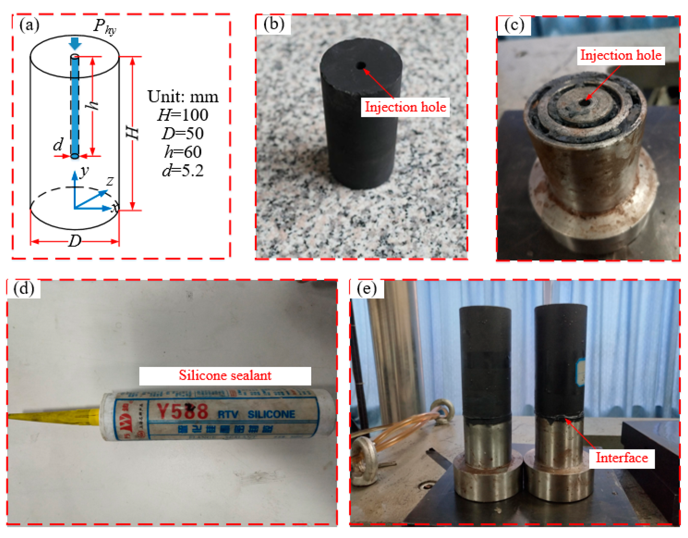
2.1. Specimen Preparations

Shale specimens for hydraulic fracturing experiments were obtained from the Longmaxi Formation of Pengshui County, China. The BP of shale reservoirs in this area is well developed, whose texture can be observed clearly, as shown in Figure 2.

The angle between the drilling orientation and the bedding planes is the anisotropic angle ($\theta$). According to the method of International Society For Rock Mechanics (ISRM), the shale cylindrical specimens with seven different anisotropic angles (Φ 50 mm, θ = 0°, 15°, 30°, 45°, 60°, 75° and 90°) were drilled with a diamond hollow using the XGZS-200 vertical coring machine, as shown in Figure 3a,b. The DQ1-4 automatic rock cutting machine was used to cut the cylindrical specimen with a length of 100 mm. The upper and lower planes of the specimen were smoothed to ensure that the parallelism within ±0.5 mm and the flatness within ±0.03 mm. Processed specimens were sealed with tape to avoid the bursting during the experiment process, as shown in Figure 3c. The mechanical properties parameters of the shale samples are presented in

Table 1. Mechanical properties parameters of the shale.

Parameters	Axis Parallel to the Layer			Axis Vertical to the Layer
	0°-1	0°-2	Mean	90°-1	90°-2	Mean
Uniaxial compression strength, UCS/MPa	102.14	110.57	106.36	148.84	152.27	150.56
Elastic modulus/GPa	16.38	15.17	15.78	31.01	28.74	29.88
Poisson’s ratio	0.31	0.29	0.30	0.29	0.27	0.28
Shear modulus/GPa	6.25	5.88	6.07	12.02	11.31	11.67

.

Injection holes were drilled with a diameter of 5–6 mm and depth of 50–60 mm in the middle of processed specimens, as shown in Figure 4a,b. To facilitate the operation of experiment, the platen with a double concentric O-ring encircling the central injection port was processed for fracturing fluid injection, as shown in Figure 4c. Shale specimens were bonded tightly to the platen by silicone sealant (see Figure 4d). The cohesive composite was consolidated at natural temperature for more than 12 h, as shown Figure 4e.

2.2. Experimental Apparatus

The mechanical seepage testing system (TAW-2000) was employed in the hydraulic fracturing experiment. Figure 5 shows the hydraulic fracturing test system. This test involved four equipment systems, namely the test loading system, confining pressure control system, displacement measurement system and water injection test system.

The assembled specimens were installed on the test bench. The sensitivity of each sensor was tested first, and then shale specimens were fixed. The test should be performed under the condition of high-pressure water pump. The fracturing fluid is water. Since the instantaneous failure of the specimen can easily lead to the damage of displacement sensor or injection pressure platen, several rubber rings were fixed on the side of the specimen in addition to the tape package. Axial and circumferential deformation were measured in all hydraulic fracturing tests.

When placed in a pressure chamber, the specimen was subjected to axial and lateral confining pressure, except for the injection pressure. Among them, axial load σ_V simulated vertical far-field stress, while confining pressure σ_con presented the uniform horizontal stress. The constant confining pressure σ_con was applied under the impermeable casing pipe, while the axial compression σ_V remained constant. Both axial load σ_V and confining pressure σ_con were controlled by servo system.

Table 2. Summary of the experimental parameters of shale specimens.

No.	Anisotropic Angle θ/°	σV/MPa	σcon/MPa	∆σ/MPa	qin/mL·s−1	σpb/MPa
1	0°	20	10	10	0.1	18.61
2	15°	20	10	10	0.1	26.22
3	30°	20	10	10	0.1	40.78
4	45°	20	10	10	0.1	54.50
5	60°	20	10	10	0.1	50.24
6	75°	20	10	10	0.1	44.91
7	90°	20	10	10	0.1	39.82
8	45°	15	10	5	0.1	59.65
9	45°	25	10	15	0.1	50.36
10	75°	20	10	10	0.2	51.74
11	90°	20	10	10	0.2	47.79

lists experimental parameters of shale specimens.

The hydraulic fracturing test mainly included five steps: (1) confining pressure was set at 10 MPa by hydraulic control; (2) axial pressure was applied to the target level (e.g., σ_V = 20 MPa) by controlling the hydraulic chamber; (3) the above stress state was maintained for about 10 min; (4) the fracturing fluid was injected into the injection hole through a constant injection rate; (5) all the data were recorded simultaneously during the whole experiment process, including injection pressure and the circumferential displacement.

3. Results and Analysis

In this section, the evolution and morphology of HF in shale specimens are described by injection pressure curves and circumferential displacements monitored in the experiment. In addition, the propagation pattern of shale specimens and the width of HF in a certain time are also analyzed.

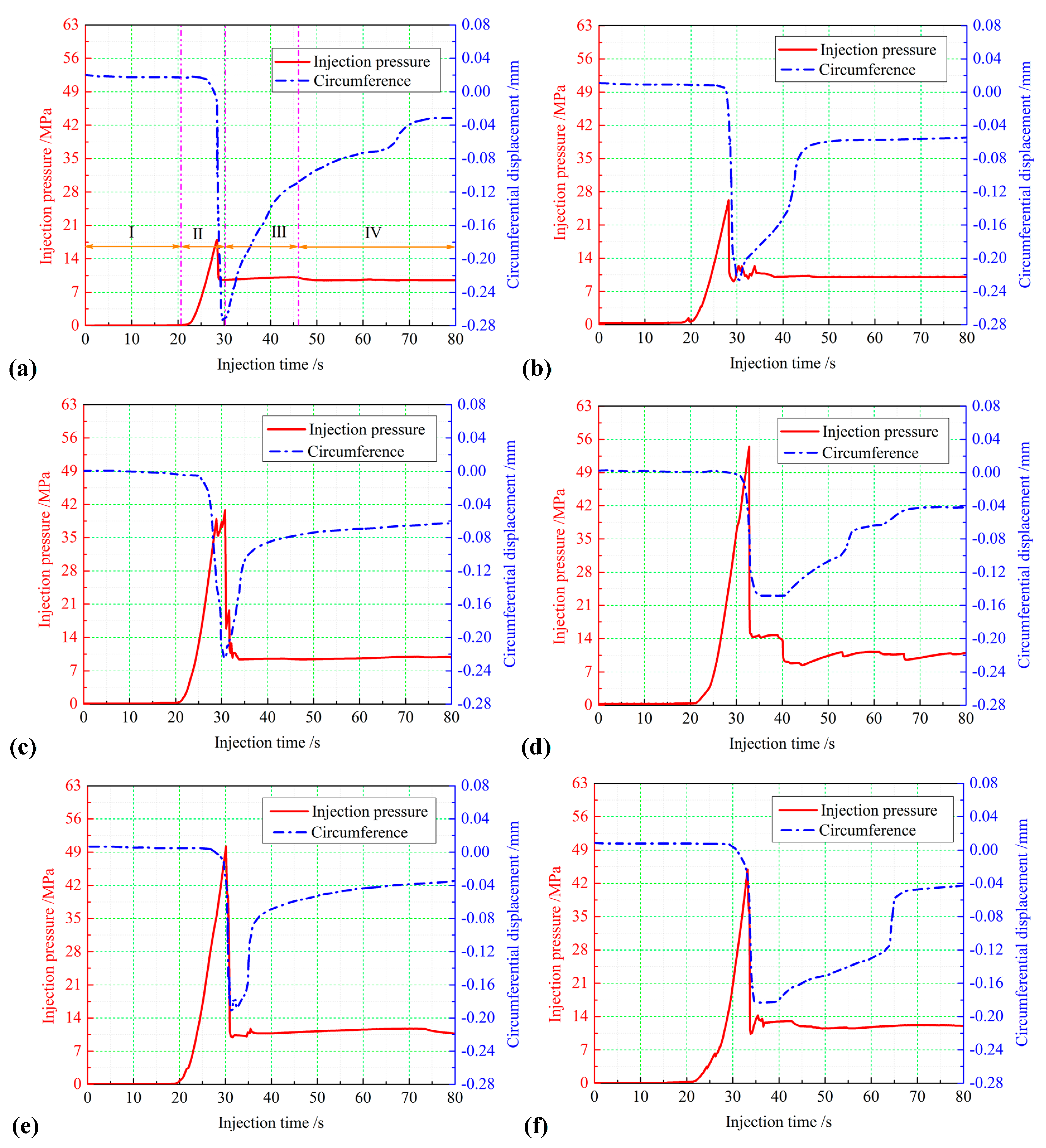
3.1. Breakdown Pressure

When the injection rate is 0.1 mL/s and deviator stress is 10 MPa, the injection pressure and circumferential displacement curves of anisotropic shale specimens are shown in Figure 6. According to the variation characteristics of the two curves, the fracturing process can be divided into four stages: Stage I, fluid injection stage; Stage II, pressure increase stage; Stage III, fracture closure stage; and Stage IV, pressure stability stage (Figure 6a).

At Stage I, the fracturing fluid cannot fill the whole injection hole, or cause the deformation of the shale specimen. Thus, the injection pressure and the circumferential displacement keep stable after entering to the Stage II where the fracturing fluid fills up the hole. Before reaching the breakdown pressure, the injection pressure increases rapidly in 6–7 s, the effective stress of shale specimens increases, resulting in the generation of HF and abrupt increase of the circumferential displacement. At Stage III, the shale specimens which involve HFs are continuously injected at a constant injection rate, and the injection pressure suddenly drops due to the leakage of the fracturing fluid by the new HF. However, the confining pressure remains unchanged (σ_con =10 MPa), so the circumferential displacement decreases and HF closure occurs. After entering the Stage IV, the injection pressure basically balances at 10 MPa, and the circumferential displacement changes sightly. While transitioning from Stage II to Stage III, the injection pressure curve takes a nosedive. Following the rapid drop in the injective pressure, the circumferential displacement increases dramatically. This occurs because of the generation of apparent and large-size HF. Therefore, the rapid drop here is an indicator that the specimen is completely broken. Though a small amount of HF can still grow as the injection continues, they are not the main hydraulic fractures. While conducting hydraulic fracturing experiments, if the confining pressure is not applied to the specimen, the injection pressure rapidly drops to 0 after the specimen is completely fractured. This occurs because of fluid leakage. In Figure 6, the confining pressure is applied to the specimen. In this case, after the specimen is completely fractured, the injection pressure decreases rapidly as well but it drops to a level similar to the applied axial pressure.

Figure 7 shows the breakdown pressure, circumferential displacement and fracturing efficiency of specimens with different anisotropic angles. With the increase of anisotropic angle, the breakdown pressure of shale specimen first increases and then decreases, but the circumferential displacement shows an opposite trend. In this paper, the maximum circumferential displacement caused by unit breakdown pressure represents fracturing efficiency. Therefore, the fracturing efficiency is calculated using the following equation:

$$FE=\frac{{\sigma }_{bp}}{\Delta D}$$

(1)

where FE is the fracturing efficiency, σ_bp is the breakdown pressure; ∆D is the circumferential displacement.

As shown in Figure 7, fracturing efficiency of shale specimens at θ = 0° is much higher than that under other operating conditions. The fracturing efficiency first decreases greatly and then increases slightly. Therefore, when hydraulic fracturing is carried out, and the direction of fluid injection is consistent with that of natural defects, the fracturing efficiency is the highest.

The trend of breakdown pressure and circumferential displacement is mainly caused by the following reasons. Firstly, when the hydraulic fracturing experiment on shale specimens at θ ≤ 30° is conducted, HF is easy to initiate between BP due to the low tensile strength. There is little difference between the angle of BP orientation and injection direction of fracturing fluid. Therefore, for shale specimens of θ ≤ 30°, HF rapidly propagates and coalesces after the initiating, resulting in lower breakdown pressure. Secondly, in terms of fracture mechanics, the critical stress intensity factor is closely related to the anisotropic angle. According to the relative theoretical analysis [33,34], the critical stress intensity factor increases first and then decreases with the change of the anisotropic angle, as shown in Figure 8. Higher critical stress intensity factor can produce higher injection pressure to facilitate the propagation of HF. Therefore, shale specimens have the highest breakdown pressure at θ = 45°. Finally, for shale specimens at θ = 45°, the breakdown pressure increases to the maximum, while the circumferential displacement and fracturing efficiency are the minimum. This is because, in this case, the permeability of shale specimen is the lowest, and the HF propagation and coalescence are less. The breakdown pressure is easy to be increased and the number of HF is reduced. The same conclusion has been obtained in the physical experiments in the previous studies [35].

When the fracturing direction aligns with the anisotropic angle, HF can propagate more easily. As a result, the shale specimens fail at a low breakdown pressure. Therefore, FE is at the highest level. However, please note that this does not necessarily mean that fracturing along the bedding plane is optimal in hydraulic fracturing design. Though FE is high, HF cannot produce highly intensive fracture networks. As a result, fracture treatment cannot be satisfactorily made to the shale matrix. Therefore, less shale gas desorbs from the matrix and the transport channel is not favorably opened up.

3.2. Propagation Modes

Compared with specimens without BP, the macro-fracture propagation modes of anisotropic shale specimens become more complex and diverse. Figure 9 shows the typical HF propagation patterns of shale specimens. The red line represents the HF, and the green line represents the anisotropic orientation.

Although HF propagates along the maximum principal stress (the direction of axial load σ_V) and crosses BP, there are obvious differences. For the specimen without BP, HF, which is called crossing pattern, is generally symmetrical and perpendicular to the specimen. In this fracturing experiment, the propagation pattern of crossing HF also exists (Figure 9a). Besides, there may be several crossing HFs (Figure 9b), or HFs can possibly divert when crossing BP (Figure 9c). In the Figure 9d, two symmetrical crossing HFs are generated during the hydraulic fracturing experiment, and HF also propagates along the BP direction (such HF is called bedding-plane HF). By the comparison of Figure 9a,b, when the injection rate and deviator stress remain unchanged, and the anisotropic angle θ is larger, namely the angle between BP and the maximum principal stress is larger, HF tends to cross BP and cross the whole specimen. By the comparison of Figure 9c,d, when deviator stress is small, HF extends to propagate along BP at the same injection rate and anisotropic angle θ.

When the anisotropic angle θ is smaller, crossing HF through the shale specimen is not generated, some of specimens propagate directly along BP (Figure 9e). In the fractured specimen, natural defects also cause eccentric initiation of the shale specimen, resulting in uneven propagation of the hydraulic fracture (Figure 9f). It can be concluded that the anisotropy generated by BP has an important influence on the propagation pattern of HF.

If the normal stress acting on the BP is small, the fracturing fluid can flow into BP and cause the shear slip. According to the linear friction criterion, the critical stress of shear slip in BP is:

$$\left|{\tau }_{na}\right|>{\tau }_0+f_n({\sigma }_{na}-P_0)$$

(2)

where ${\tau }_{na}$ is the tangential stress of BP; ${\tau }_0$ is the inherent shear strength of BP; $f_n$ is the friction coefficient of BP; and ${\sigma }_{na}$ is the normal stress of BP.

The normal and shear stresses in BP are calculated as follows:

$${\tau }_{na}=\frac{{\sigma }_V-{\sigma }_{con}}{2}\sin 2{\psi }_{HF}$$

(3)

$${\sigma }_{na}=\frac{{\sigma }_V+{\sigma }_{con}}{2}+\frac{{\sigma }_V-{\sigma }_{con}}{2}\cos 2{\psi }_{HF}$$

(4)

where ${\psi }_{HF}$ is the approaching angle, namely the interaction angle between HF and BP.

When HF and BP interact, the pore pressure $P_0$ is calculated as [36]:

$$P_0=S_h+P_{\sigma }$$

(5)

where $P_{\sigma }$ is the treatment stress of pore structure change.

When the pore pressure of BP exceeds the normal stress, HF crosses BP to generate new fractures:

$$P_0>{\sigma }_{na}$$

(6)

By substituting Equations (3) and (4) into Equation (5), the effect factors of interaction between HF and BP is obtained:

$$P_{\sigma }>\frac{(S_H-S_h)\cdot (1-\cos 2{\psi }_{HF})}{2}$$

(7)

It can be seen from Equation (7) that, increasing the approaching angle ${\psi }_{HF}$ can increase the possibility that HF crosses BP. The larger the approaching angle, the more difficult the fracturing fluid propagates along the direction of BP extension. Meanwhile, increasing the deviator stress $\Delta \sigma$ can increases the possibility that HF crosses BP, and it is easy for HF to propagate along the maximum principal stress direction. The larger the deviator stress, the more difficult the HF diverts, and the easier to cross BP by HF. Through theoretical analysis and physical experiment verification, the conclusion is consistent.

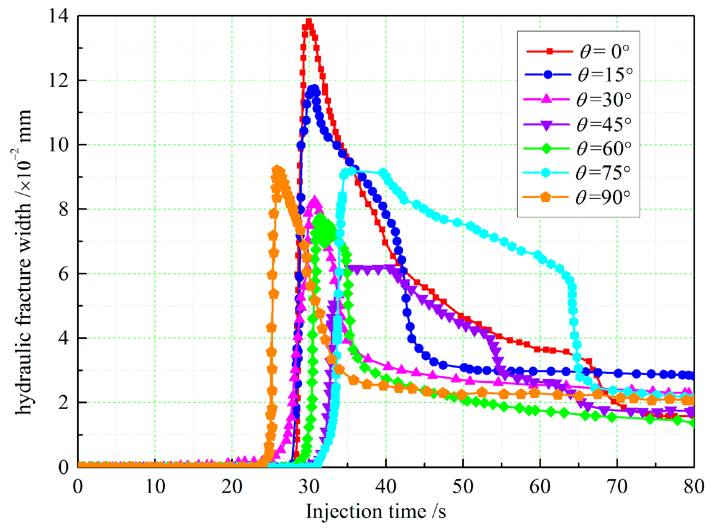
3.3. Fracture with Evolution

HFN formed by the interaction of HF and BP is the main pathway of shale gas migration, so HF is an important parameter to evaluate the effect of hydraulic fracturing. The accurate measurement of HF width helps to select particle size of proppant. In addition, by monitoring injection pressure and circumferential displacement, it is found that the elastic deformation of rocks can be negligible, compared to the initiation and propagation of HF. Therefore, the width of HF in the fracturing process can be calculated according to the deformation of circumferential displacement and the HF shape [37], as shown in Figure 10.

The width of HF can be calculated as:

$$W_f=\frac{\Delta D}{n_{f1}+n_{f2}\cdot \cos \theta }$$

(8)

where $\Delta D$ is the variation in the monitored circumference; $n_{f1}$ is the number of crossing HF; and $n_{f2}$ is the number of bedding-plane HF. It should be noted that $\Delta D$ is an approximation that ignores the tortuosity.

Figure 11 shows the evolution curve of HF width with injection time. Similar to the injection pressure, the evolution curve of HF width can be divided into four stages. Once the fracturing fluid fills the injection hole and starts to pressurize, the circumferential strain increases rapidly, and the HF width reaches its maximum at about 5 s. At this time, macroscopic HF initiates when the shale specimen is fractured. Generally, the maximum width of HF occurs before and after the injection pressure reaches its peak. After that, the width of HF decreases dramatically, and there are several fluctuations during this period. This phenomenon is mainly caused by the sudden generation of HF. When HF propagates to the boundary, the fracturing fluid gradually leaks off. Finally, HF is closed until the experimental stress state reaches the equilibrium.

Table 3. Summary of the hydraulic fracture width evolution.

No	θ/°	Failure Mode	Maximum Width/×10−2 mm	Ultimate Width/×10−2 mm	Closure ×10−2 mm	Closure Proportion/%
1	0	Bedding-plane	13.82	3.16	10.66	77.13
2	15	Bedding-plane	11.74	5.46	6.28	53.49
3	30	Bedding-plane + Crossing	8.26	6.27	1.99	24.09
4	45	Bedding-plane + Crossing	6.17	4.26	1.91	30.96
5	60	Crossing	7.74	3.43	4.31	55.68
6	75	Crossing	9.18	4.28	4.90	53.38
7	90	Crossing	9.21	4.14	5.07	55.05

shows the statistics of HF width evolution. When θ is small (θ = 0° or 15°), the propagation pattern of shale specimens is bedding-plane mode. In these specimens, although the maximum width of HF is large, the closure proportion is also high, since HF propagates along the BP during the hydraulic fracturing process. When the bedding is activated, once the fracturing fluid leaks off, the bedding is closed as the original path. With the increase of θ (θ = 30° or 45°), the propagation pattern changes from bedding-plane mode to the combination of bedding-plane and crossing mode. In this case, although the maximum width of HF is generally low, the ultimate width of HF is relatively high. Therefore, the closure proportion is low, the effect of fracturing treatment is the best with the lowest requirement for the proppant. When θ is very large (θ ≥ 60°), the maximum width of HF reaches a trough. The closure proportion of HF is also very high, and the fracturing effect is the worst. The magnitude in Figure 11 was compared against the reference [38]. The comparison demonstrates that the magnitude in Figure 11 are in good agreement with the data in the reference.

4. Discussion

The selected samples are outcrops. In general, outcrop specimens do affect experimental results due to reasons such as weathering and the absence of primitive stress. However, outcrop specimens do not have an effect on the properties associated with hydraulic fracturing. It is difficult to sample the shale underground. In this case, the outcrop specimens have a minor degree of weathering, thereby having small effects on the results. This paper deals with the laboratory study of the hydraulic fracturing. The derived findings cannot be directly applied to industry design. However, the presented experimental methodology and the research contents can guide industry practice.

We did draw a comparison between the HF width in the experiment and that in the field. The HF width in the experiment is at the micron scale, while the HF width in the field is at the centimeter scale (2–5 cm). Therefore, the HF width varies significantly from the experiment to the field. There are the following reasons to be aware of: (1) The shale reservoir in the experiment differs from that in the field in sizes. The shale reservoir in the experiment is the standard cylindrical specimen, while the in-situ reservoir is much larger and contains a number of naturally occurring fractures (NF). (2) Reservoirs with different sizes result in different injection flows. The injection flow in the experiment is measured in milliliter while the injection flow in the field is measured in tonnage. The difference is huge. (3) There is also a huge difference in fracturing duration. Field fracturing experiments take a much longer time than laboratory experiments. Therefore, the derived HF width cannot represent the real-life scenario. However, laboratory experiments can still deliver a host of values. Different from the laboratory experiments, field experiments require the consideration of issues such as extraction efficiency and environmental contamination.

As a fracturing fluid, slickwater has a smaller viscosity coefficient than clear water. From the perspective of hydraulic fracturing, fracturing fluid with large viscosity coefficient results in poor fracturing effect as it does not contribute to the generation of complex HFN. Slickwater and clear water exhibit similar behavior when interacting with temperature and pressure. However, slickwater has obvious disadvantages compared with clear water. First, slickwater performs poorly in carrying the proppant. Though slickwater contributes to the formation of complex HFN, it fails to let the proppant play an effective role in opening up the transport channel. Second, slickwater is easy to leak off. In addition, slickwater contains some chemicals. The leakage poses a threat to underground aquifers. Moreover, in the case of slickwater, after HFN formation, shale gas cannot desorb easily from the shale matrix, thereby failing to meet the production yield requirements. Therefore, clear water is currently used as the main source of the fracturing fluid. We intend to investigate further into this topic in our future studies.

5. Conclusions

Hydraulic fracturing treatment greatly improves the efficiency of shale gas exploitation and extraction, contributing to the industrial production of unconventional oil and gas. Shale is a typical transversely isotropic material. The layered structure of shale results in the complicated mechanical behavior. In the process of hydraulic fracturing, complex bedding structure is the basis for the formation of hydraulic fracture network (HFN). In this paper, the effect of shale anisotropy on hydraulic fracture (HF) propagation behavior is studied through hydraulic fracturing experiments. The conclusions can be drawn as follows:

(1)

Anisotropy has a significant effect on the breakdown pressure, circumferential displacement and fracturing efficiency of shale specimens. When anisotropic angle θ ≤ 15°, since of the small tensile strength of shale specimens, HF can easily initiate and propagate between BP, resulting in a smaller breakdown pressure. Especially for shale specimens at θ = 0°, the fracturing efficiency is much higher than other operating conditions. When θ = 45°, the critical stress intensity factor increases the strength of shale specimen, leading to the rapid increase of breakdown pressure, while the circumferential strain and fracturing efficiency are relatively low. When θ ≥ 60°, the breakdown pressure decreases, but it is still higher than that at smaller θ.

(2)

Due to the effect of bedding plane, two symmetrical HF cannot be formed in some shale specimens. When HF and bedding plane (BP) interact, increasing deviator stress and approaching angle help HF cross BP. When θ ≤ 15°, the bedding-plane mode is ubiquitous in all shale reservoirs. While θ ranged from 30°–45°, a comprehensive propagation pattern of bedding-plane and crossing is presented. When θ ≥ 60°, the HFN pattern changes from comprehensive mode to crossing mode. The propagation mode obtained from physical tests and the theoretical analysis are mutually verified.

(3)

With the increase of θ, the maximum width of HF decreases first and then increases gradually, but the ultimate width of HF shows an opposite trend. Therefore, the closure proportion is the highest when the propagation pattern is the bedding-plane mode (θ ≤ 15°). The closure proportion of the crossing mode is the second. Only when the bedding-plane and crossing HF occur simultaneously, the closure proportion is the smallest, the fracturing effect is the best with the lowest requirement for the proppant. The results can provide some basic data for the design in hydraulic fracturing of tight oil/gas reservoirs.

References

1. Wang, Q.; Lu, H.; Shen, C.; Liu, J.; Peng, P.A.; Hsu, C.S. Impact of Inorganically Bound Sulfur on Late Shale Gas Generation. Energy Fuels 2014, 28, 785–793. [Google Scholar] [CrossRef] [Green Version]
2. Zhu, H.Y.; Guo, J.C.; Zhao, X.; Lu, Q.; Luo, B.; Feng, Y.C. Hydraulic Fracture Initiation Pressure of Anisotropic Shale Gas Reservoirs. Geomech. Eng. 2014, 7, 403–430. [Google Scholar] [CrossRef]
3. Lu, Y.; Ge, Z.; Yang, F.; Xia, B.; Tang, J. Progress on the Hydraulic Measures for Grid Slotting and Fracking to Enhance Coal Seam Permeability. Int. J. Min. Sci. Technol. 2017, 27, 867–871. [Google Scholar] [CrossRef]
4. Jiang, T.; Zhang, J.; Wu, H. Experimental and Numerical Study on Hydraulic Fracture Propagation in Coalbed Methane Reservoir. J. Nat. Gas Sci. Eng. 2016, 35, 455–467. [Google Scholar] [CrossRef]
5. Zhu, S.Y.; Du, Z.M.; Li, C.L.; Salmachi, A.; Peng, X.L.; Wang, C.W.; Yue, P.; Deng, P. A Semi-Analytical Model for Pressure-Dependent Permeability of Tight Sandstone Reservoirs. Transp. Porous Media 2018, 122, 235–252. [Google Scholar] [CrossRef]
6. Li, Y.; Yang, S.; Zhao, W.; Li, W.; Zhang, J. Experimental of Hydraulic Fracture Propagation Using Fixed-Point Multistage Fracturing in a Vertical Well in Tight Sandstone Reservoir. J. Pet. Sci. Eng. 2018, 171, 704–713. [Google Scholar] [CrossRef]
7. Chen, M.; Sun, Y.; Fu, P.; Carrigan, C.R.; Lu, Z.; Tong, C.H. Surrogate-Based Optimization of Hydraulic Fracturing in Pre-Existing Fracture Networks. Comput. Geosci. 2013, 58, 69–79. [Google Scholar] [CrossRef]
8. Zou, Y.; Zhang, S.; Ma, X.; Zhou, T.; Zeng, B. Numerical Investigation of Hydraulic Fracture Network Propagation in Naturally Fractured Shale Formations. J. Struct. Geol. 2016, 84, 1–13. [Google Scholar] [CrossRef]
9. Ezulike, D.O.; Dehghanpour, H. A Model for Simultaneous Matrix Depletion into Natural and Hydraulic Fracture Networks. J. Nat. Gas Sci. Eng. 2014, 16, 57–69. [Google Scholar] [CrossRef]
10. Liu, Z.; Chen, M.; Zhang, G. Analysis of the Influence of a Natural Fracture Network on Hydraulic Fracture Propagation in Carbonate Formations. Rock Mech. Rock Eng. 2014, 47, 575–587. [Google Scholar] [CrossRef]
11. Zolfaghari, A.; Dehghanpour, H.; Holyk, J. Water sorption behaviour of gas shales: I. Role of clays. Int. J. Coal Geol. 2017, 179, 130–138. [Google Scholar] [CrossRef]
12. Zolfaghari, A.; Dehghanpour, H.; Xu, M. Water sorption behaviour of gas shales: II. Pore size distribution. Int. J. Coal Geol. 2017, 179, 187–195. [Google Scholar] [CrossRef]
13. Bohloli, B.; De Pater, C.J. Experimental Study on Hydraulic Fracturing of Soft Rocks: Influence of Fluid Rheology and Confining Stress. J. Pet. Sci. Eng. 2006, 53, 1–12. [Google Scholar] [CrossRef]
14. Zhang, D.; Ranjith, P.G.; Perera, M.S.A. The Brittleness Indices Used in Rock Mechanics and their Application in Shale Hydraulic Fracturing: A Review. J. Pet. Sci. Eng. 2016, 143, 158–170. [Google Scholar] [CrossRef]
15. Kolykhalov, I.V.; Martynyuk, P.A.; Sher, E.N. Modeling Fracture Growth Under Multiple Hydraulic Fracturing Using Viscous Fluid. J. Min. Sci. 2016, 52, 662–669. [Google Scholar] [CrossRef]
16. Wang, Y.; Li, X.; Tang, C.A. Effect of Injection Rate on Hydraulic Fracturing in Naturally Fractured Shale Formations: A Numerical Study. Environ. Earth Sci. 2016, 75, 935. [Google Scholar] [CrossRef]
17. Hofmann, H.; Babadagli, T.; Zimmermann, G. Numerical Simulation of Complex Fracture Network Development by Hydraulic Fracturing in Naturally Fractured Ultratight Formations. J. Energy Resour. Technol. 2014, 136, 42905. [Google Scholar] [CrossRef]
18. Osiptsov, A.A. Fluid Mechanics of Hydraulic Fracturing: A Review. J. Pet. Sci. Eng. 2017, 156, 513–535. [Google Scholar] [CrossRef]
19. Fan, T.G.; Zhang, G.Q. Laboratory Investigation of Hydraulic Fracture Networks in Formations with Continuous Orthogonal Fractures. Energy 2014, 74, 164–173. [Google Scholar] [CrossRef]
20. Dehghan, A.N.; Goshtasbi, K.; Ahangari, K.; Jin, Y. Experimental Investigation of Hydraulic Fracture Propagation in Fractured Blocks. Bull. Eng. Geol. Environ. 2015, 74, 887–895. [Google Scholar] [CrossRef]
21. Gu, H.; Weng, X.; Lund, J.B.; Mack, M.G.; Ganguly, U.; Suarez-Rivera, R. Hydraulic Fracture Crossing Natural Fracture at Nonorthogonal Angles: A Criterion and its Validation. SPE Prod. Oper. 2012, 27, 20–26. [Google Scholar] [CrossRef]
22. Wang, W.; Li, X.; Lin, B.; Zhai, C. Pulsating Hydraulic Fracturing Technology in Low Permeability Coal Seams. Int. J. Min. Sci. Technol. 2015, 25, 681–685. [Google Scholar] [CrossRef]
23. Olson, J.E.; Taleghani, A.D. Modeling Simultaneous Growth of Multiple Hydraulic Fractures and their Interaction with Natural Fractures. In Proceedings of the SPE Hydraulic Fracturing Technology Conference, The Woodlands, TX, USA, 19–21 January 2009; Society of Petroleum Engineers: Richardson, TX, USA, 2009. [Google Scholar]
24. Wang, Y.; Li, X.; Zhang, B. Analysis of Fracturing Network Evolution Behaviors in Random Naturally Fractured Rock Blocks. Rock Mech. Rock Eng. 2016, 49, 4339–4347. [Google Scholar] [CrossRef]
25. Zhang, L.; Zhou, J.; Braun, A.; Han, Z. Sensitivity Analysis on the Interaction Between Hydraulic and Natural Fractures Based on an Explicitly Coupled Hydro-Geomechanical Model in PFC2D. J. Pet. Sci. Eng. 2018, 167, 638–653. [Google Scholar] [CrossRef]
26. Wanniarachchi, W.A.M.; Ranjith, P.G.; Perera, M.S.A.; Rathnaweera, T.D.; Zhang, D.C.; Zhang, C. Investigation of effects of fracturing fluid on hydraulic fracturing and fracture permeability of reservoir rocks: An experimental study using water and foam fracturing. Eng. Fract. Mech. 2018, 194, 117–135. [Google Scholar] [CrossRef]
27. Mohammadnejad, T.; Andrade, J.E. Numerical modeling of hydraulic fracture propagation, closure and reopening using XFEM with application to in-situ stress estimation. Int. J. Numer. Anal. Methods Geomech. 2016, 40, 2033–2060. [Google Scholar] [CrossRef]
28. Chong, Z.; Li, X.; Hou, P.; Chen, X.; Wu, Y. Moment Tensor Analysis of Transversely Isotropic Shale Based on the Discrete Element Method. Int. J. Min. Sci. Technol. 2017, 27, 507–515. [Google Scholar] [CrossRef]
29. Dubey, R.K.; Gairola, V.K. Influence of Structural Anisotropy on the Uniaxial Compressive Strength of Pre-Fatigued Rocksalt From Himachal Pradesh, India. Int. J. Rock Mech. Min. Sci. 2000, 6, 993–999. [Google Scholar] [CrossRef]
30. Song, H.; Jiang, Y.; Elsworth, D.; Zhao, Y.; Wang, J.; Liu, B. Scale Effects and Strength Anisotropy in Coal. Int. J. Coal Geol. 2018, 195, 37–46. [Google Scholar] [CrossRef]
31. Taniguchi, T.; Mitsumata, T.; Sugimoto, M.; Koyama, K. Anisotropy in Elastic Modulus of Hydrogel Containing Magnetic Particles. Phys. A Stat. Mech. Appl. 2006, 370, 240–244. [Google Scholar] [CrossRef]
32. Collet, O.; Gurevich, B.; Madadi, M.; Pervukhina, M. Modeling Elastic Anisotropy Resulting from the Application of Triaxial Stress. Geophysics 2014, 79, C135–C145. [Google Scholar] [CrossRef]
33. Wang, X.; Shi, F.; Liu, H.; Wu, H. Numerical Simulation of Hydraulic Fracturing in Orthotropic Formation Based on the Extended Finite Element Method. J. Nat. Gas Sci. Eng. 2016, 33, 56–69. [Google Scholar] [CrossRef]
34. Asadpoure, A.; Mohammadi, S. Developing New Enrichment Functions for Crack Simulation in Orthotropic Media by the Extended Finite Element Method. Int. J. Numer. Methods Eng. 2007, 69, 2150–2172. [Google Scholar] [CrossRef]
35. Pan, R.; Cheng, Y.; Yuan, L.; Yu, M.; Dong, J. Effect of Bedding Structural Diversity of Coal on Permeability Evolution and Gas Disasters Control with Coal Mining. Nat. Hazards 2014, 73, 531–546. [Google Scholar] [CrossRef]
36. Warpinski, N.R.; Teufel, L.W. Influence of Geologic Discontinuities on Hydraulic Fracture Propagation. J. Pet. Technol. 1987, 39, 209–220. [Google Scholar] [CrossRef]
37. He, J.; Lin, C.; Li, X.; Zhang, Y.; Chen, Y. Initiation, Propagation, Closure and Morphology of Hydraulic Fractures in Sandstone Cores. Fuel 2017, 208, 65–70. [Google Scholar] [CrossRef]
38. Zolfaghari, A.; Dehghanpour, H.; Ghanbari, E.; Bearinger, D. Fracture characterization using flowback salt-concentration transient. SPE J. 2016, 21, 233–244. [Google Scholar] [CrossRef]
Figure 1. Fracture geometries and fluid flow patterns with bedding plane.
Energies 12 00976 g001
Figure 2. (a) Shale sampling location, (b) sampled layer, (c) processed disc specimen, and (d) microscopic detail of the shale bedding plane.
Energies 12 00976 g002
Figure 3. Sampling process of shale with anisotropic angles; (a) diagram of sampling orientation; (b) specimen preparation process; (c) final specimens.
Energies 12 00976 g003
Figure 4. Specimen processing for the hydraulic fracturing experiment; (a) Specimen size; (b) Shale specimen after drilling; (c) Platen with a double concentric O-ring encircling the central injection port; (d) Silicone sealant; (e) Installed specimens.
Energies 12 00976 g004
Figure 5. Hydraulic fracture testing system.
Energies 12 00976 g005
Figure 6. Injection pressure and circumferential displacement versus injection time in rock mass with different anisotropic angles; (a) θ = 0°; (b) θ = 15°; (c) θ = 30°; (d) θ = 45°; (e) θ = 60°; (f) θ = 75°; (g) θ = 90°.
Energies 12 00976 g006aEnergies 12 00976 g006b
Figure 7. Comparison among hydraulic fracturing results at different anisotropic angles.
Energies 12 00976 g007
Figure 8. Changes of critical stress intensity factor at different anisotropic angles [33,34].
Energies 12 00976 g008
Figure 9. Typical fracture propagation mode in hydraulic fracturing test on shale; (a) at θ = 75°, ∆σ = 10 MPa and qin = 0.2 mL/s; (b) at θ = 90°, ∆σ = 10 MPa and qin = 0.2 mL/s; (c) at θ = 45°, ∆σ = 15 MPa and qin = 0.1 mL/s; (d) at θ = 45°, ∆σ = 5 MPa and qin = 0.1 mL/s; (e) at θ = 30°, ∆σ = 10 MPa and qin = 0.1 mL/s; (f) at θ = 60°, ∆σ = 10 MPa and qin = 0.1 mL/s.
Energies 12 00976 g009
Figure 10. Schematic diagram of fracture width calculation.
Energies 12 00976 g010
Figure 11. Hydraulic fracture width evolution with injection time in shale cores.
Energies 12 00976 g011