Thin Conductor Modelling Combined with a Hybrid Numerical Method to Evaluate the Transferred Potential from Isolated Grounding System

Abstract

Grounding systems are essential parts of substations and power generation stations. The evaluation of transferred potentials from an active grounding system to other passive ones or to any near conductors is an important aspect to be considered, because transferred potentials may cause serious and fatal events. Moreover, it is an intrinsic issue of the Smart Grid where the ground systems of the power and ICT systems could be close to each other. Therefore, the estimation of the transferred potential is necessary at grounding system design stage for people safety and electric components safeguard. Numerical methods are the best choice to perform a truthful estimation, especially when large and complex grounding systems have to be designed. However, this task is complicated by the “unbounded” nature of the electromagnetic field and by the presence of components of extremely different size in the analysis domain. In this paper, an efficient hybrid finite element method is applied for the accurate and fast computation of transferred earth potentials from grounding systems. Moreover, the small dimensions of the components in the analysis domain are taken into account by the use of one-dimensional finite elements inserted in the tetrahedral mesh. It is worth mentioning the additional advantage of obtaining the electric potential on the earth surface without any post-processing operation.

1. Introduction

Grounding systems (GSs) are very important components of electric systems in substations and power plants, as well as in any civil, commercial, and industrial building, because they are essential for human safety [1] and equipment safeguard [2].

IEEE Standard 80 and IEC 479-1 establish the body current limits to be met when designing a GS [3]. Such limits involve permissible touch-and-step voltages [4], which must be accurately evaluated.

The presence of passive GSs, over ground metallic elements (e.g., train tracks, fences), as well as underground ones (e.g., pipelines), in the vicinity of an active GS induces a modification of the electromagnetic field due to the active GS, as well as transferred potentials (TPs) that, in turn, may cause safety issues. The values of TPs must also be evaluated to verify the limit satisfaction outside the active GS in order to take suitable countermeasures. In this regard, the standard EN 50522 provides some qualitative indications [5]. In this paper, TPs from isolated GSs are considered, while the TPs through conductors connected to the active GS [6,7] are not.

TPs from an active GS to a passive one or to metallic components in the proximity of the GS always occur, except for in a few cases [8]. Very often, metal rails are present in large substations and power plants to facilitate the transportation of transformer equipment and fuel. These rails may transfer hazardous potentials around the switchyard area when a ground fault occurs [9].

Moreover, TPs may damage equipment in the neighborhood of windfarm turbines, which have increasing diffusion as green energy power generators [10]. TPs may lead to undesired interfering effects in special power systems, such as hospital and data centers [11].

More in general, the study of the TPs is an intrinsic issue in smart grids due to the high integration of ICT and power systems [12]. In urban areas, TPs in buried metallic parts, such as water and gas pipes, tramway tracks, and building foundations, are of particular concern because they involve worsening safety when there are floating conductors near an active GS [13].

During line maintenance, a de-energized line may be subject to uncontrollable transfer of the grid potential from other energized lines. Grounding the line at source end for personnel protection during maintenance involves greater hazard due to TP into this temporary GS from the active GS of other energized lines when they are faulted [14].

Commercial software tools usually used for GS analysis present limitations in evaluating the safety risk due to the transfer of potential out of a substation grounding system. Numerical methods based on the finite element method (FEM) are the best choice for the estimation of GS behavior, since they enable to account for more physical phenomena and to provide accurate results [15]. In such a context, the effectiveness of hybrid numerical methods in GS analysis has already been proved [16,17].

The advantages that derive from the use of hybrid numerical methods for TP evaluation are presented in this paper. More specifically, the FEM-DBCI (Dirichlet boundary condition iteration) is effectively applied to TP evaluation. Furthermore, the real dimension and conductivity of the GS grid is considered by properly treating conductor slenderness, then the accuracy worsening due to some simplifications that are usually adopted in GS modelling is discussed. Finally, it is worth to note that, due to the possibility of decomposing the analysis domain in separated subdomains, the FEM-DBCI outperform other numerical methods, especially when the TP in large domains has to be evaluated.

2. Overview of Finite Element Analysis for the Evaluation of the Potential Transfer from Isolated Grounding Systems

The influence of buried metallic objects on the performance of power system grounds and the transferred earth potentials in power systems were initially performed by means of empirical methods. More accurate results have only been obtained by means of analytical methods implemented in computer programs since the 1970s [5,9,18,19,20].

In this context, circuit method based on simplified formulas has been also adopted [21]. On the other hand, these methods involve a high computational costs or unrealistic results when the section of conductors increases, as well as unpredictable margin of error [22,23].

The FEM provides better results for the computation of GS behavior, it enables to take into account for stratified soils, and it can consider different types and configurations of the GS, regardless of the size, length, type and shapes of the electrodes [12]. An additional benefit of FEM is that the electric potential distribution on the earth surface is directly provided as part of the solution.

FEM has been used to compute the main quantities related to the GS by using the domain truncation combined with analytical expressions [24,25] or by means of spatial transformation techniques [26]. An optimal size of the 3D finite elements near the GS conductors (modeled as 1D elements) is determined as a function of their radius [27]. The distribution of the potential of a GS belonging to an L-shape building has been simulated by means of finite difference method (FDM) in [28].

FEM and FDM are useful for solving close-boundary value problems. When the problem exhibits open boundaries, as in the case of a GS analysis, these methods imply very poor accuracy to computational cost ratios since the discretization of a large domain is necessary in order to obtain acceptable results [29,30]. These drawbacks are exacerbated when evaluating the TPs due to the very wide analysis domain to be considered. Moreover, the use of FDM is almost complex when the GS grid is irregular.

A numerical technique based on the transformation of the differential equations underlying the physical phenomena onto an equivalent boundary integral equation and the subsequent application of the boundary element method (BEM) has been proposed in References [31,32]. The method of moments (MoM) has also been effectively adopted for obtaining a solution for the integral equations [33].

These approaches overcome the aforementioned limitations of empirical and analytical methods as well as the difficulties of FEM and FDM. On the other, the soil is considered to be homogeneous, or with limited inhomogeneity, and the size and resistivity of the conductors are neglected. The first limitation has been overcome by using a layered soil model in the application of BEM while maintaining the other simplifications [34,35]. In the case of multiple layer models, the application of the “method of images” enables relevant improvement in convergence rate while managing the maximum admissible error [36], but the computation of the boundary integrals remains a very hard task due to the presence of singularity and of Green functions expressed by series.

Moreover, although the BEM well describes the GS geometry and is suitable to cope with the unbounded nature of the problem, it suffers from a cumbersome post-processing phase with high computational effort and limited accuracy.

The hybrid FEM-DBCI numerical method combines the benefits of the FEM and boundary integral methods. It has been used for evaluating the GS behavior [17] without considering TPs. Moreover, in Reference [17] it was presented as an accurate approach to properly consider both the conductivity and the size of each conductor of a GS. Such an approach has the very welcome feature of avoiding the thickening of the mesh of the regions around and inside the conductors. Such an advantage is obtained by modelling the conductors with 1D finite elements and merge the unknowns of these elements with those of the 3D ones adopted to discretize the soil. This approach is very useful in TP analysis, considering the presence of other conductors. For this reason, it has been combined in this work with the aforesaid hybrid numerical method.

3. The FEM-DBCI Method

In Figure 1, two GSs are shown buried in unbound soil. For the sake of simplicity, we assume that the soil is satisfactorily modelled as two-layer medium, in which the overlying layer has finite depth h and conductivity σ₁ whereas the underlying layer is an infinite half space of conductivity σ₀ (with σ₀ > σ₁). With the aim of studying the TP phenomenon, we consider that one GS (active) is energized at voltage V₀, whereas the other GS (passive) is floating.

In order to apply the FEM-DBCI method for the computation of the electrical potential v and the current density J around the GSs, a truncation boundary Γ_T is selected enclosing all the GSs and the non-homogeneous objects localized around them, if any. Since the two GSs are separated by a great distance, the boundary Γ_T is constituted by two detached surfaces (see the red dashed lines in Figure 1).

The Laplace equation

$$\nabla \cdot \left(\mathsf{\sigma }\nabla \mathrm{v}\right)=0$$

(1)

holds in the bounded domain D, whose boundaries are Γ_T and the soil surface Γ₀. On Γ₀, a homogeneous Neumann conditions ∂v/∂n=0 holds, whereas an unknown Dirichlet boundary condition is assumed to hold on Γ_T, so that the FEM can be applied to the bounded domain D.

The soil inside D is discretized by means of tetrahedral finite elements, whereas the conductors of the GSs are modelled as 1D finite elements in addition to the 3D ones. A modified conductivity (in Sm)

$${\mathsf{\sigma }}_{\mathrm{mod}}={\mathsf{\eta }}_{\mathrm{s}}{\mathsf{\sigma }}_{\mathrm{c}}{\mathrm{S}}_{\mathrm{c}}$$

(2)

is attributed to these 1D elements, where σ_c is the metal conductivity (in S/m), S_c is its cross section area (in m²), and η_s is a numerical coefficient, which is set to 1, 1/2 or 1/4, according to the position of the conductor with respect to symmetry planes. For a 1D element, say E, the triple integral relative to its stiffness matrix is transformed into a line integral:

$${\mathrm{s}}_{\mathrm{mn}}={\displaystyle {\iiint }_{\mathrm{E}}\nabla {\mathsf{\alpha }}_{\mathrm{m}}\cdot \nabla {\mathsf{\alpha }}_{\mathrm{n}}\mathrm{d}\mathrm{x}\mathrm{d}\mathrm{y}\mathrm{d}\mathrm{z}}={\mathsf{\eta }}_{\mathrm{s}}{\mathrm{S}}_{\mathrm{c}}{\displaystyle {\int }_{\mathrm{L}}\nabla {\mathsf{\alpha }}_{\mathrm{m}}\cdot \nabla {\mathsf{\alpha }}_{\mathrm{n}}\mathrm{d}\mathrm{s}}$$

(3)

where α_m and α_n are the shape functions of the m-th and n-th nodes, respectively, and L is the segment relative to the 1D finite element E.

By introducing the following universal values [37]:

$${\mathrm{s}}_{\mathrm{m}\mathrm{n}}^{*}={\displaystyle {\int }_0^1\frac{\mathrm{d}{\mathsf{\alpha }}_{\mathrm{m}}}{\mathrm{d}\mathsf{\xi }}\frac{\mathrm{d}{\mathsf{\alpha }}_{\mathrm{n}}}{\mathrm{d}\mathsf{\xi }}\mathrm{d}\mathsf{\xi }}$$

(4)

where ξ is the local (non-dimensional) coordinate along the segment, the line integral in Equation (3) can be actually computed by means of such values as:

$${\mathrm{s}}_{\mathrm{m}\mathrm{n}}={\mathsf{\eta }}_{\mathrm{s}}{\mathrm{S}}_{\mathrm{c}}\mathrm{L}{\mathrm{s}}_{\mathrm{m}\mathrm{n}}^{*}$$

(5)

In this way, along the conductors of the GSs, we can observe a variation of the potential. For the energized GS the Dirichlet condition v = V₀ is imposed on its point at the soil surface.

By applying the FEM to the bounded domain, the following algebraic system is obtained:

$$\mathbf{A}\mathbf{v}={\mathbf{b}}_0-{\mathbf{A}}_{\mathrm{T}}{\mathbf{v}}_{\mathrm{T}}$$

(6)

where v is the array of the potential values at the nodes lying inside D and along Γ₀, v_T is the array of the potential values at the nodes lying on Γ_T; A, and A_T, are sparse matrices of geometrical coefficients; b₀ is the known term array due to the assigned voltages.

The unknown Dirichlet condition on the truncation boundary is expressed by means of the integral equation [38]:

$$\mathrm{v}(\mathrm{P})={\displaystyle {\iint }_{{\Gamma }_{\mathrm{M}}}\left(\mathrm{v}(\mathrm{P}{}^{\prime })\frac{\partial \mathrm{G}(\mathrm{P},\mathrm{P}{}^{\prime })}{\partial \mathrm{n}{}^{\prime }}-\mathrm{G}(\mathrm{P},\mathrm{P}{}^{\prime })\frac{\partial \mathrm{v}(\mathrm{P}{}^{\prime })}{\partial \mathrm{n}{}^{\prime }}\right)\mathrm{d}\mathrm{S}{}^{\prime }}$$

(7)

where Γ_M is a closed surface (see the blue dotted line in Figure 1) enclosing all the conductors and non-homogeneities, but strictly enclosed by Γ_T. The integration surface Γ_M is conveniently selected homologous to Γ_F and constituted by triangular faces of tetrahedral elements. Often, two layers of elements are inserted in between Γ_M and Γ_T. Other more suitable ways to choose the Γ_M surface are described in Reference [39].

In Equation (7) P and P′ are points lying on Γ_T and Γ_M, respectively, n’ is the outward normal unit vector to Γ_M and G(P, P′) is the two-layer soil Green’s function [17]. In this case, the use of the two-layer (or multi-layer) soil Green’s function does not complicate the evaluation of the integral equation (Equation (7)) because the integration surface Γ_M is separated from the truncation one Γ_T, and no singularities arise. For this reason, in the presence of multi-layered soil, it is preferable to avoid the use of the BEM, even if it is combined with FEM [40], while the FEM-DBCI method is more suitable [41].

In numerical form, the integral equation (Equation (10)) reads:

$${\mathbf{v}}_{\mathrm{T}}=\mathbf{F}\mathbf{v}$$

(8)

where F is a dense rectangular matrix having non null columns only for the nodes involved in the integral equation, that is, for the nodes of the tetrahedra external to Γ_M and having a face lying on it.

The FEM-DBCI global algebraic system is constituted by Equations (6) and (8). This system can be solved by means of the generalized minimal residual (GMRES) solver, used as described in Reference [42]. Alternatively, by taking advantage of the fact that the integral equation (Equation (8)) is explicit with respect to the array v_T, the following iterative procedure may be used: (1) start from an arbitrary initial guess for v_T; (2) solve the FEM equation (Equation (6)) for v by means of the conjugate gradient (CG) solver; (3) use the DBCI equation (Equation (8)) to improve v_T; (4) iterate these steps until convergence takes place [38]. FEM-DBCI has been implemented in ELFIN, a numerical code developed by the authors for electromagnetic research [43].

4. Numerical Results

This section firstly presents a simple example to verify the accuracy for numerical solution, then the computation of TP from an active GS to a near passive one, then the problem of TP from a GS to a metal rail has been treated.

4.1. A Single Rod Vertically Buried in a Homogeneous Soil

The first example is a very basic one and consists of a single rod vertically buried in a homogeneous soil. For this simple system, an analytical formula (9) for the grounding resistance is available:

$${\mathrm{R}}_{\mathrm{g}}=\frac{\ln \frac{4\mathrm{L}}{\mathrm{r}}-1}{2\mathsf{\pi }\mathsf{\sigma }\mathrm{L}}$$

(9)

where L is the rod length, r its radius and $\mathsf{\sigma }$ the soil conductivity. Considering a rod with L = 10 m and r = 5 mm, buried in a soil with $\mathsf{\sigma }$ = 0.01 S/m, Equation (9) gives a value of grounding resistance R_g = 12.71 Ω.

There are many factors that affect the solution accuracy when 3D computer aided design is adopted 44. In case of GS analysis, it is known that the accuracy of the finite element solution is strongly affected by the grid size in the vicinity of the rod [27]. Hence, in order to verify the accuracy of the FEM-DBCI method with 1D elements, different numerical evaluations of the grounding resistance are performed, modifying the discretization of the rod and of its immediate neighborhood. The rod is discretized by means of 1D elements while the first-order tetrahedra have been adopted in the 3D domain. The parameter s = L/N_s, where N_s is the number of subdivisions of the rod, is varied from 0.1 m to 0.0125 m, doubling the number N_s each simulation. The unbounded soil is truncated by means of a fictitious boundary Γ_F placed at a distance d = 3 m from the rod. Symmetry is exploited by reducing the analysis domain to the octant x > 0, y > 0, and z < 0. Homogeneous Neumann conditions on the symmetry planes are assumed. The integration surface Γ_M is selected at distance s from the rod.

Table 1. Grounding resistance R_g and computing effort in terms of CPU times and unknowns vs. different values of parameter s.

s (m)	Rg (Ω)	Tetrahedra	Nodes	CPU Time (s) 1
0.1000	9.366	3667	1060	0. 02
0.0500	10.62	7793	2227	0.06
0.0250	11.46	14249	3989	0.20
0.0125	12.69	29575	8307	0.81

¹ Intel^© Core i7-5600, 2.6 GHz. 8 Gb RAM.

shows the results, putting in evidence the correct behavior of the proposed numerical procedure: In fact, the error on the value of the computed grounding resistance decreases if a finer mesh is adopted in the proximity of the rod. Moreover, the use of 1D elements allows to obtain a very accurate value of the ground resistance with a low computational cost. Other simulations were carried out moving away the fictitious boundary but no significant difference was observed in the results, besides an expected growth of the computing time.

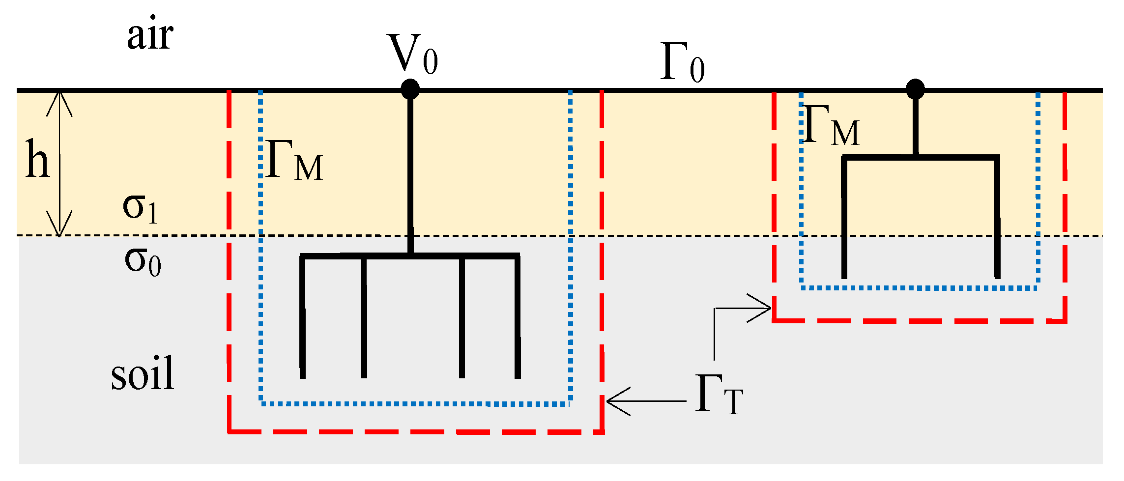
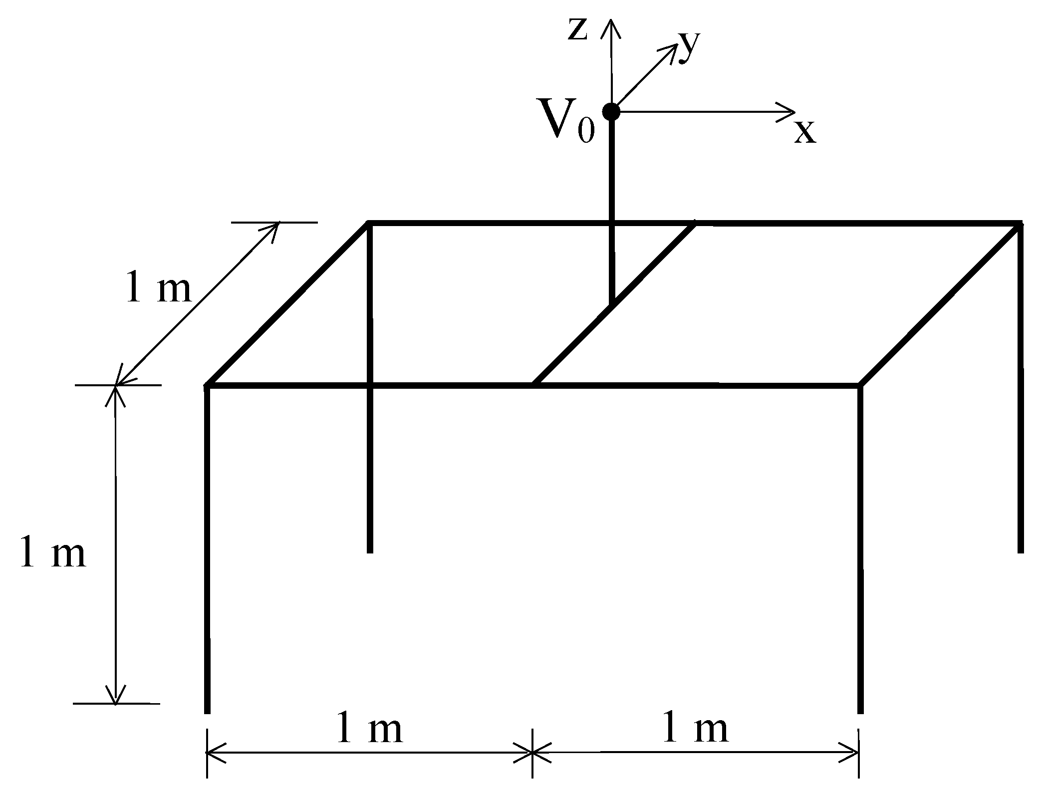
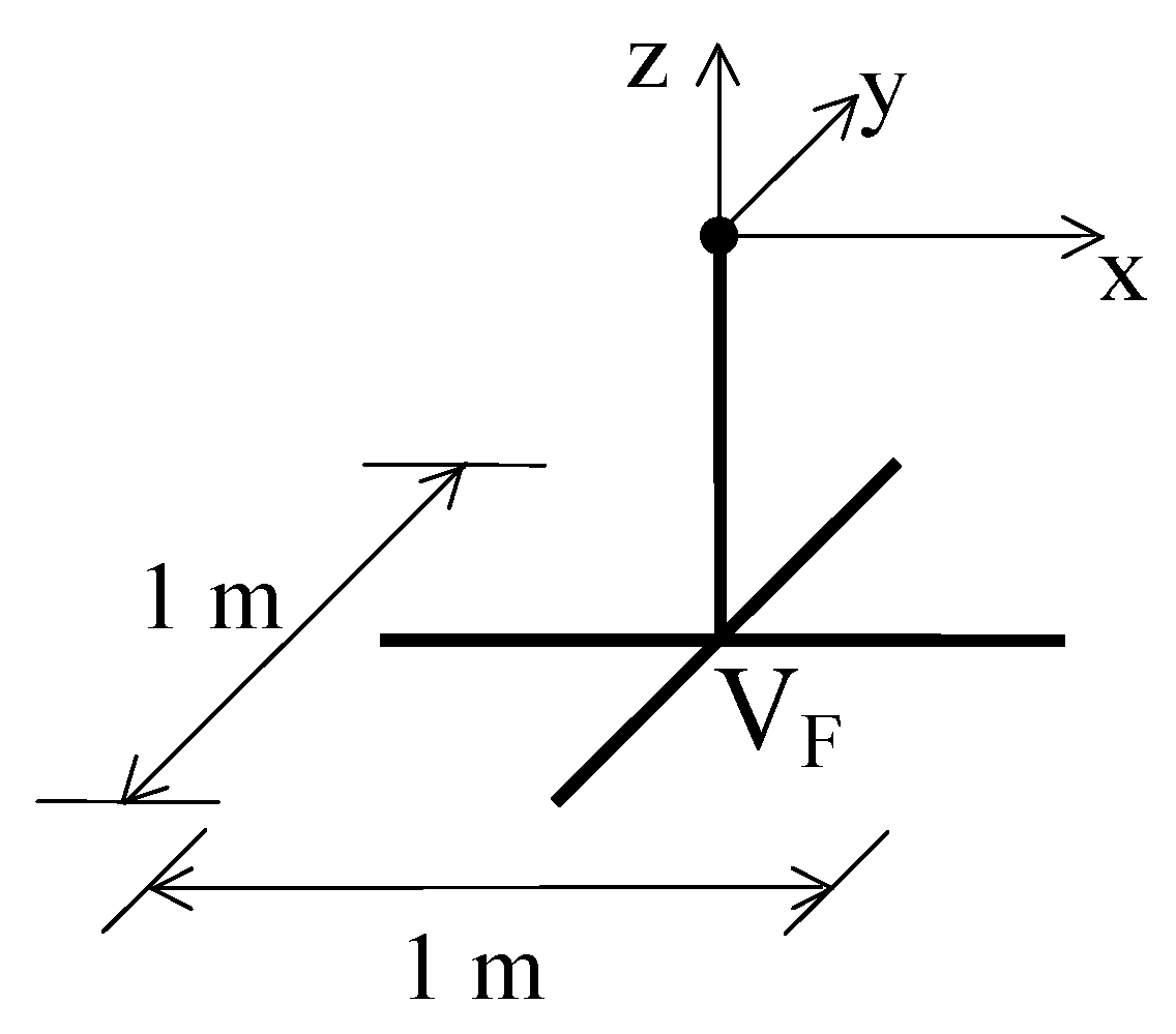
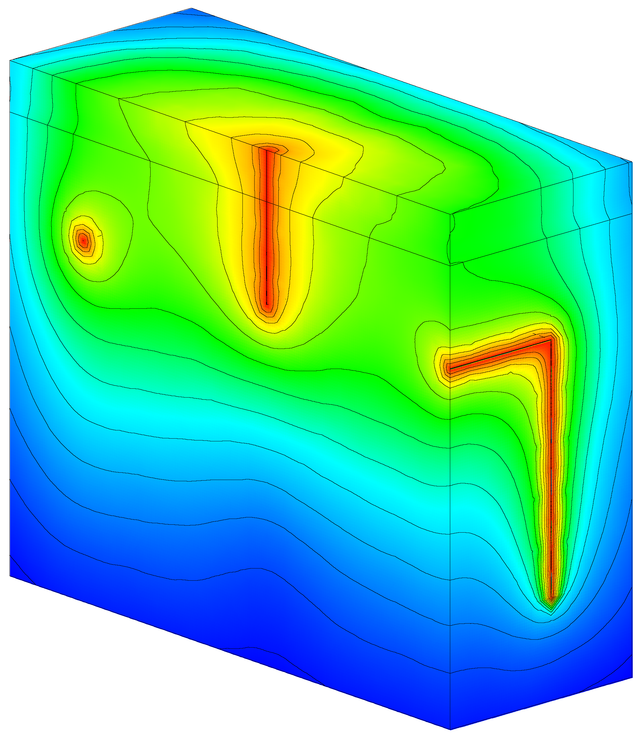
4.2. Transferred Potential from an Active to a Passive Grounding System

Figure 2 shows the geometry of the active GS where there are two equal squares, with dimension 1 m × 1 m, buried parallel with the soil surface at 0.6 m in depth. They present a rod of length 0.6 m that connects them with the soil surface and four other vertical rods, 1 m in length, at its corners. They are steel (σ_c = 7.0⋅10⁶ S/m) conductors and the radius, r_c, of their circular cross section is equal to 1 cm. The voltage of the active GS is set to V₀ = 100 V, hence the voltage across the passive GS may be considered directly as the percentage of TP to such a GS since the problem under study is linear.

The intersection between the ground surface and the rod connecting the GS with such a surface is adopted as origin of the reference coordinate system used for the analysis. The z axis has been chosen orthogonal with the soil surface while the y axis has been chosen parallel with the common side between the two squares.

A cross with dimension 1 m × 1 m buried at 0.6 m in depth and belonging to a plane parallel to the ground surface constitutes the passive GS. It is connected to the ground surface through a vertical rod of 0.6 m placed at the cross intersection. The arms of the cross are aligned along the x- and y-axes, far away 15 m from the center of the first system in the x direction. Figure 3 shows the passive GS

Both xz and xy coordinate planes are symmetry planes for the active and passive GSs according to the chosen reference coordinate system and GSs position.

The soil is modelled as an unbounded medium with two strays: the upper one with depth h = 20 cm and conductivity σ₁ = 3.33⋅10⁻⁴ S/m while the bottom has conductivity σ₀ = 0.05 S/m.

The symmetry in the analysis domain enable the consideration of only a quarter, thus strongly reducing the computational effort necessary to perform the simulation. More specifically, the considered analysis sub-domain is the portion with y > 0, z < 0. The reduction is obtained by setting homogeneous Neumann conditions on the symmetry planes y = 0 and z = 0. The unbounded soil in such sub-domain is truncated by means of a fictitious boundary Γ_F constituted of two parallelepipedal boxes of sizes 2.8 m × 1.4 m × 2.0 m and 1.8 m × 0.9 m × 1.0 m, respectively for the active and passive GS. The integration surface Γ_M is selected homologous to Γ_F, at a distance of 0.2 m.

Second-order tetrahedra have been adopted to discretise the two detached octants, that is, the upper and lower part of the sub-domain. More specifically, 23,660 tetrahedra have been considered for the former while 56,160 for the latter. The analysis converges in four iterations being the stopping criteria a tolerance of 10⁻⁴ per cent for the CG solver and 10⁻² per cent for the GMRES. Figure 4 shows the contours of the electrical potential in the xz symmetry plane and on Γ_F around the active GS. The floating potential at the centre of the cross of the passive GS is about V_F= 4.32 V. In other words, the TP to the passive GS is the 4.32% of the voltage appearing at the ground surface of the active GS.

4.3. Transferred Potential from an Active to a Metal Rail

The active GS of Figure 3 is considered while the passive system is a massive steel rail with a length of 4 m aligned along the y-axis with cross section of 10 cm × 20 cm. The bar is buried in the soil being the upper side aligned with the soil surface. The middle point of the bar is far away 15 m from the center of the GS in the x direction. The soil is modelled as an upper layer of depth h = 20 cm and σ₁ = 3.33⋅10⁻⁴ S/m and a below unbounded medium of conductivity σ₀ = 0.05 S/m. The two detached subdomains are discretized by means of tetrahedral finite elements of the second order, for a total 52301 and 81154 nodes. In Figure 5, the contours of the potential are drawn on the soil surface around the bar. The mean value of the electric potential of the bar is about 5.7 V. Once again, this means the TP at the bar is 5.7% of the active GS.

5. Conclusions

In this paper, the hybrid method FEM-DBCI has been applied to evaluate the transferred potentials from an active grounding system. Firstly, the advantages that derive from the use of such hybrid numerical methods for grounding system have been recalled and then have been shown in case of known grounding resistance. Then, two numerical examples have been solved and the results have highlighted the accuracy of the solution provided by the method.

Due to the hybrid nature of the FEM-DBCI, the possibility of decomposing the analysis domain in separated subdomains has been exploited, avoiding the discretization of the large volume of soil between the active and the floating conductors. Moreover, the implementation of 1D elements to model the grounding grid and the rods, that had a very small section compared with the analysis domain, hugely decreased the number of tetrahedra in the mesh. In this way, applying FEM-DBCI dramatically reduced the computing time.

References

1. Di Silvestre, M.L.; Favuzza, S.; Mangione, S.; Mineo, L. On the interconnections of HV-MV stations to global grounding systems. IEEE Trans. Ind. Appl. 2019, 55. [Google Scholar] [CrossRef]
2. Phayomhom, A.; Sirisumrannukul, S.; Kasirawat, T.; Puttarach, A. Safety design improvement of grounding system by compression ratio and ground rod layout methods: Case study of metropolitan electricity authority’s power distribution system. Presented at the CIGRE Session 45—45th International Conference on Large High Voltage Electric Systems, Paris, France, 24–30 August 2014. [Google Scholar]
3. Lee, C.H.; Meliopoulos, A.S. A comparison of IEC 479-1 and IEEE Std 80 on grounding safety criteria. Proc. Natl. Sci. Counc. Repub. China Part A Phys. Sci. Eng. 1999, 23, 612–621. [Google Scholar]
4. Lee, C.H. Safety assessment of bulk and traction supply substations in Taipei rail transit systems. IEEE Trans. Power Deliv. 2004, 19, 1078–1084. [Google Scholar] [CrossRef]
5. Freschi, F.; Mitolo, M.; Tartaglia, M. Interferences phenomena between separate grounding systems. IEEE Trans. Ind. Appl. 2014, 50, 2853–2860. [Google Scholar] [CrossRef]
6. Mangione, S.; Mineo, L. Safety concerns on ground fault application transfer phenomenon in HV installations. In Proceedings of the IEEE Symposium on Product Compliance Engineering, Longmont, CO, USA, 22–23 October 2007. [Google Scholar] [CrossRef]
7. Chou, C.; Liu, C. Assessment of risks from ground fault transfer on closed-loop HV underground distribution systems with cables running in a common route. IEEE Trans. Power Deliv. 2013, 28, 1015–1023. [Google Scholar] [CrossRef]
8. Bhang, B.G.; Kim, G.G.; Cha, H.L.; Kim, D.K.; Choi, J.H.; Park, S.Y.; Ahn, H.K. Design methods of underwater grounding electrode array by considering inter-electrode interference for floating PVs. Energies 2018, 11, 982. [Google Scholar] [CrossRef]
9. Garrett, D.L.; Wallace, K.A. A critical analysis of grounding practices for railroad tracks in electric utility stations. IEEE Trans. Power Deliv. 1993, 8, 90–96. [Google Scholar] [CrossRef]
10. Lorentzou, M.I.; Hatziargyriou, N.D.; Papadias, B.C. Analysis of wind turbine grounding systems. In Proceedings of the 10th Mediterranean Electrotechnical Conference. Information Technology and Electrotechnology for the Mediterranean Countries, Lemesos, Cyprus, 29–31 May 2000; pp. 936–939. [Google Scholar] [CrossRef]
11. Parise, G.; Parise, L.; Martirano, L. Identification of global grounding systems: The global zone of influence. IEEE Trans. Ind. Appl. 2015, 51, 5044–5049. [Google Scholar] [CrossRef]
12. Martin, A.R. Safety issues and damage to equipment with both Smart Grid and home network connections. In Proceedings of the IEEE Symposium on Product Compliance Engineering Proceedings, Boston, MA, USA, 5–7 May 2010; pp. 1–5. [Google Scholar] [CrossRef]
13. Pons, E.; Colella, P.; Tommasini, R.; Napoli, R.; Montegiglio, P.; Cafaro, G.; Torelli, F. Global earthing system: Can buried metallic structures significantly modify the ground potential profile. IEEE Trans. Ind. Appl. 2015, 51, 5237–5246. [Google Scholar] [CrossRef]
14. Suresh, K.; Paranthaman, S. Transferred potential—A hidden killer of many linemen. IEEE Trans. Ind. Appl. 2015, 51, 2691–2699. [Google Scholar] [CrossRef]
15. Leschert, D.; Iwasykiw, G.; Derworiz, R. Substation grounding transfer of potential case studies. IEEE Trans. Ind. Appl. 2016, 52, 661–667. [Google Scholar] [CrossRef]
16. Trlep, M.; Hamler, A.; Jesenik, M.; Stumberger, B. The FEM-BEM analysis of complex grounding systems. IEEE Trans. Magn. 2003, 39, 1155–1158. [Google Scholar] [CrossRef]
17. Aiello, G.; Alfonzetti, S.; Rizzo, S.A.; Salerno, N. Efficient analysis of grounding systems by means of the hybrid FEM–DBCI method. IEEE Trans. Ind. Appl. 2015, 51, 5159–5166. [Google Scholar] [CrossRef]
18. Dawalibi, F.; Mukhedkar, D. Transferred earth potentials in power systems. IEEE Trans. Power Appar. Syst. 1978, PAS-97, 90–101. [Google Scholar] [CrossRef]
19. Simpson, I.B.K.; Bensted, D.J.; Dawalibi, F.; Blix, E.D. Computer analysis of impedance effects in large grounding systems. IEEE Trans. Ind. Appl. 1987, IA-23, 490–497. [Google Scholar] [CrossRef]
20. Wu, A.Y.; Meliopoulos, A.P. Analysis of ground potential gradients around power substations. In Proceedings of theAnnual Technical Conference on Pulp and Paper Industry, Seattle, WA, USA; 1990; pp. 56–66. [Google Scholar] [CrossRef]
21. Ala, G.; Favuzza, S.; Francomano, E.; Giglia, G.; Zizzo, G. On the distribution of lightning current among interconnected grounding systems in medium voltage grids. Energies 2018, 11, 771. [Google Scholar] [CrossRef]
22. Navarrina, F.; Colominas, I.; Casteleiro, M. Why do computer methods for grounding analysis produce anomalous results? IEEE Trans. Power Deliv. 2003, 18, 1192–1202. [Google Scholar] [CrossRef] [Green Version]
23. Brenna, M.; Foiadelli, F.; Longo, M.; Zaninelli, D. Particular grounding systems analysis using FEM models. In Proceedings of the International Conference on Harmonics and Quality of Power, Ljubljana, Slovenia, 13–16 May 2018. [Google Scholar] [CrossRef]
24. Guemes, J.A.; Hernando, F.E. Method for calculating the ground resistance of grounding grids using FEM. IEEE Trans. Power Deliv. 2004, 19, 595–600. [Google Scholar] [CrossRef]
25. Guemes, J.A.; Hernando-Fernandez, F.E.; Rodriguez-Bona, F.; Ruiz-Moll, J.M. A practical approach for determining the ground resistance of grounding grids. IEEE Trans. Power Deliv. 2006, 21, 1261–1266. [Google Scholar] [CrossRef]
26. Trlep, M.; Hamler, A.; Hribernik, B. The analysis of complex grounding systems by FEM. IEEE Trans. Magn. 1998, 34, 2521–2524. [Google Scholar] [CrossRef]
27. Silva, V.C.; Martinho, L.B.; Cardoso, J.R.; Filho, M.L.P.; Verardi, S.L.L. Efficient modeling of thin wires in a lossy medium by finite elements applied to grounding systems. IEEE Trans. Magn. 2011, 47, 966–969. [Google Scholar] [CrossRef]
28. Chen, J.; Liao, W.; Wang, Y.; Liu, X. Finite-difference analysis of the potential distribution around an L-shape building base under the measurement of grounding resistance. In Proceedings of the Asia-Pacific International Conference on Lightning, Chengdu, China, 1–4 November 2011. [Google Scholar] [CrossRef]
29. Talaat, M.; Farahat, M.A.; Essa, M.A.; Maowwad, M.S. Simulation of the electric field and the GPR resulting from vertical-driven rods earthing system in a multi-layers earth structure. Measurement 2019, 132, 387–401. [Google Scholar] [CrossRef]
30. Liu, J.; Lin, G.; Wang, F.; Li, J. The scaled boundary finite element method applied to electromagnetic field problems. IOP Conf. Ser. Mater. Sci. Eng. 2014, 10, 012245. [Google Scholar] [CrossRef]
31. Colominas, I.; Navarrina, F.; Casteleiro, M. Boundary element formulation for the analysis of transferred potentials in electrical installations. Adv. Eng. Softw. 2004, 35, 601–607. [Google Scholar] [CrossRef] [Green Version]
32. Colominas, I.; Navarrina, F.; Casteleiro, M. Analysis of transferred earth potentials in grounding systems: A BEM numerical approach. IEEE Trans. Power Deliv. 2005, 20, 339–345. [Google Scholar] [CrossRef]
33. Faleiro, E.; Pazos, F.J.; Asensio, G.; Denche, G.; García, D.; Moreno, J. Interaction between interconnected and isolated grounding systems: A case study of transferred potentials. IEEE Trans. Power Deliv. 2015, 30, 2260–2267. [Google Scholar] [CrossRef]
34. Colominas, I.; Navarrina, F.; Casteleiro, M. Numerical simulation of transferred potentials in earthing grids considering layered soil models. IEEE Trans. Power Deliv. 2007, 22, 1514–1522. [Google Scholar] [CrossRef]
35. Zildzo, H.; Muharemovic, A.; Turkovic, I.; Matoruga, H. Numerical calculation of floating potentials for large earthing system. In Proceedings of the XXII International Symposium on Information, Communication and Automation Technologies, Bosnia, Serbia, 29–31 October 2009; pp. 1–6. [Google Scholar] [CrossRef]
36. Colominas, I.; París, J.; Guizán, R.; Navarrina, F.; Casteleiro, M. Numerical modeling of grounding systems for aboveground and underground substations. IEEE Trans. Ind. Appl. 2015, 51, 5107–5115. [Google Scholar] [CrossRef]
37. Silvester, P.P.; Ferrari, R.L. Finite Elements for Electrical Engineers, 3rd ed.; Cambridge University Press: Cambridge, UK, 1996. [Google Scholar]
38. Aiello, G.; Alfonzetti, S.; Coco, S. Charge iteration: A procedure for the finite element computation of unbounded electrical fields. Int. J. Numer. Methods Eng. 1994, 37, 4147–4166. [Google Scholar] [CrossRef]
39. Aiello, G.; Alfonzetti, S.; Salerno, N. Improved Selection of the Integration Surface in the Hybrid FEM-DBCI Method. IEEE Trans. Magn. 2010, 46, 3357–3360. [Google Scholar] [CrossRef]
40. Alfonzetti, S.; Salerno, N. A Non-Standard Family of Boundary Elements for the Hybrid FE-BE Method. IEEE Trans. Magn. 2009, 45, 1312–1315. [Google Scholar] [CrossRef]
41. Aiello, G.; Alfonzetti, S.; Borzì, G.; Rizzo, S.A.; Salerno, N. A Comparison between Hybrid Methods: FEM-BEM versus FEM-DBCI. Int. J. Comput. Math. Electr. Electron. Eng. (COMPEL) 2013, 32, 1901–1911. [Google Scholar] [CrossRef]
42. Aiello, G.; Alfonzetti, S.; Borzì, G.; Dilettoso, E.; Salerno, N. A GMRES Iterative Solution of FEM-BEM Global Systems in Skin Effect Problems. Int. J. Comput. Math. Electr. Electron. Eng. (COMPEL) 2008, 27, 1286–1295. [Google Scholar] [CrossRef]
43. Aiello, G.; Alfonzetti, S.; Borzì, G.; Salerno, N. An Overview of the ELFIN Code for Finite Element Research in Electrical Engineering. In Software for Electrical Engineering Analysis and Design IV; Wessex Institute of Technology Press: Southampton, UK, 1999; pp. 143–152. [Google Scholar]
44. Beirão, P.J.B.F.N.; Malça, C.M.S.P.; Felismina, R.P. Influence of design parameters on the structural and fatigue behaviors of a floating point wave energy converter. AIMS Energy 2017, 5, 209–223. [Google Scholar]
Figure 1. An active GS in the vicinity of another passive GS embedded in a two-layer soil.
Energies 12 01210 g001
Figure 2. Three-dimensional geometry of the active GS.
Energies 12 01210 g002
Figure 3. Three-dimensional geometry of the passive GS.
Energies 12 01210 g003
Figure 4. Contours of the potential around the active GS.
Energies 12 01210 g004
Figure 5. Contours of the potential around the metal rail.
Energies 12 01210 g005