Article

Renewable Energy Utilization Analysis of Highly and Newly Industrialized Countries Using an Undesirable Output Model

1
Department of Industrial Engineering and Management, National Kaohsiung University of Science and Technology, Kaohsiung 80778, Taiwan
2
Department of Electrical Engineering, Technological University of the Philippines Taguig, Taguig 1630, Philippines
3
Department of Mechanical Engineering, National Kaohsiung University of Science and Technology, Kaohsiung 80778, Taiwan
*
Authors to whom correspondence should be addressed.
Energies 2020, 13(10), 2629; https://doi.org/10.3390/en13102629
Submission received: 13 May 2020 / Revised: 19 May 2020 / Accepted: 20 May 2020 / Published: 21 May 2020
(This article belongs to the Collection Energy Economics and Policy in Developed Countries)

Abstract

:
In the fight against climate change, the utilization of renewable energy resources is being encouraged in every country all over the world to lessen the emissions of greenhouse gases. However, not all countries are able to efficiently utilize these resources, and instead of providing solutions, the inefficient use of renewable energy may lead to even more damage to the environment. Data from eight countries belonging to the highly industrialized countries (HIC) group and nine from newly industrialized countries (NIC) group were used to evaluate the energy utilization of these groups. Factors such as total renewable energy capacity, the labor force, and total energy consumption were considered to be the input factors, while, CO2 emission and gross domestic product are the output factors. These factors were used to calculate efficiency scores of every country from 2013 to 2018 using the undesirable output model of Data envelopment analysis (DEA). The grey prediction model was also used to measure the forecasted values of the input and output factors for the year 2019 to 2022, and measure again the future efficiency scores of the HICs and NICs. The combination of grey prediction and DEA undesirable output model made this paper unusual and the most appropriate method in dealing with data that contains both desired and undesired outputs. The results show that the United Kingdom, Germany, France, and the United States continuously top the efficiency ranking among the HIC group, with a perfect 1.0 efficiency score from 2013 to 2022. Russia demonstrates the lowest score of 0.1801 and is expected to perform the same low-efficiency score in the future. Within the NIC group, Indonesia can be highlighted for performing with perfect efficiency starting from the year 2015 and even through 2022. Other NICs are performing at a very low-efficiency, with scores ranging from 0.2278 to 0.2734 on average, with Turkey displaying the lowest rank. This study recommends some useful strategies to improve the utilization of renewable energy resources such as improvements in the political and legal structure surrounding their use and regulation, tax incentives or exemptions to private power producers to encourage shifting away from conventional energy production, partnerships with non-governmental and international organizations that can provide assistance in managing renewable energies, strengthening of the energy sector’s research and development activities and long-term strategic plans for the development in renewable energy with considerations to the social, environmental, and economic impact on each country.

1. Introduction

Global warming, as it is called, is simply the heating up of the atmosphere attributed mainly to the greenhouse effect caused by the rising concentrations of carbon dioxide, chlorofluorocarbons (CFCs), and other air pollutants. This extreme phenomenon is the primary reason for the climate change that is considered to be an environmental crisis. During the United Nations Framework Convention on Climate Change, several state parties agreed to pursue efforts to reduce this century’s average increase of the Earth’s temperature from 2 degrees Celsius to 1.5 degrees Celsius. The consensus entered force last November 2016 and is referred to as the Paris Agreement [1]. One foreseen solution is to slowly transform from conventional energy production based on fossil fuel combustion to renewable energy resources. Fuel combustion is a traditional way to generate electric power through the burning of coal and fossil fuels. Many countries are dependent on this practice. Even some developed ones are major contributors to the presence of CO2 in the atmosphere caused by this process [2].
In the fight against climate change, other nations are now making use of different renewable energy sources. In this way, they can lessen the use of CO2-emitting methods in the production of electricity which is very essential to human living standards. Renewable energies are sources of energy which are continuously being replenished naturally by the Earth itself. These energies can be obtained straight from the Sun (solar power and thermal), wind power, hydroelectric power, tidal or wave energy, and geothermal and biomass, but the transition to these energy sources can be difficult and costly. Though many potential benefits can ensue, there are also some technical limitations that must be considered. Also, instead of providing an additional solution to the climate change problem, the improper utilization of renewable energy may lead to more damage to the environment. These environmental damages may be caused by the disadvantages of using renewable energies such as air pollution caused by biomass burning, corrosion problems when using geothermal energy, risk of flooding in the communities surrounding a hydropower plant, negative impact on marine wildlife in using marine energy, and impact on the environmental landscape of using solar and wind energies [3].
There are international agencies and organizations that aim to provide guidance and assistance to those countries that are making their way to the use of renewable energies. One is the International Renewable Energy Agency (IRENA) which is an association of world governments that provides support to countries as they shift to a future with sustainable energy. They also function as a primary platform for global collaboration and as an archive of policies, resources, technologies, and economic know-how on renewable energy [4]. This study will use data from IRENA, Enerdata, and the World Bank.
To evaluate the relative efficiencies of the renewable energy utilization of seventeen (17) nations belonging from highly industrialized countries group (HIC—Russia, Canada, the United States, Japan, the United Kingdom, Italy, Germany, and France) which are also being referred to as the G8 or the Group of Eight Industrialized Nations [5] and newly industrialized countries group (NIC—Turkey, Thailand, Malaysia, Indonesia, India, China, Brazil, Mexico, and South Africa) [6] is the main goal of this study. These HICs and NICs are expected to have highly developed and developing economies. The HICs and NICs are chosen by the authors to be the subject countries for this study because of their high potential in investing in renewable energies since they have more developed economies. The aim is to identify which of the countries are performing efficiently as they progress in the use of their renewable energy resources. Energy consumption has an essential effect to the country’s gross domestic product (GDP) as the ratio between the two factors affects the economic output of several countries since energy is a major input in continuous consumption of goods from energy-demanding sectors such as in production and manufacturing [7].
Three input and two output factors during the six-year periods will be considered for forecasting future values using the grey forecasting method or GM (1,1). The data from the past and the future will then be analyzed using the data envelopment analysis (DEA) undesirable output model.
The combination of these two models makes this study different from other papers, especially the use of the undesirable output model in the energy sector. This model will give consideration to the presence of good and bad outputs, treating the bad or undesired outputs as less important contrary to good outputs. This paper will make use of these two methods to evaluate the past to future efficiencies of seventeen countries.
The whole paper is divided into five sections. Reviews of previous literature related to the study are found in the Section 2. The proposed approach in forecasting future values and evaluation of efficiencies is in the Section 3. The Section 4 presents the interpretations and analyses of data gathered using GM (1,1) and the results of the DEA undesirable model. Concluding statements are described in the Section 5.

2. Literature Review

The energy sector has been a very important aspect of human life and has a strong impact on the economic, social, institutional, and environmental conditions of every country. Cirstea et al. [8] calculated the renewable energy sustainable index (RESI) using the normalization and multivariate analysis which affects the said conditions. The goal of the index is to provide a framework that can be used by the renewable energy sector’s potential investors to aid their decision making. Another study conducted by Iddrisu and Bhattacharyya [9] made use of the arithmetic mean of the four normalized indicators for the measurement of the sustainable energy development index (EDI) which was devised to evaluate, rate, and rank countries according to the calculated energy indices. Lee and Zhong [10] by using min-max normalization combined with multivariate analysis were able to draft the renewable energy responsible investment index (RERII) wherein the primary intention is to help energy investors to decide effectively and proactively and also, to establish an investment framework for energy stakeholders in developing or revising current approaches for investing in the renewable energy field. The ecological factor was considered by Schlör et al. [11] to form the sustainable development index (SDI). In their study, the methods of selecting variables, normalization, and weighting to analyze whether the German energy sector is on a sustainable development track even under the pressure of sustainability goals. A general sustainability indicator for the consumption of renewable energy resources was established by Liu [12] using weighing, quantification, and evaluation of theoretical criteria. The framework incorporated a multicriteria decision-making model (MCDM) called the analytic hierarchy process (AHP) to provide a precise measurement of sustainability. The same index model was developed beforehand by Doukas et al. [13] applying a multivariate technique called the principal component analysis (PCA) for the analysis of nine different indicators to quantitatively measure the energy sustainability of rural communities. Due to the integration of MCDM techniques in various efficiency analysis, the method has become popular to evaluate the energy sector. Štreimikienė et al. [14] combined AHP with the additive ratio assessment technique (ARAS) to analyze the environmental impact criteria and rate the electricity generation technologies in Lithuania. Another method popularly known as the Technique for Order Preference by Similarity to Ideal Solution (TOPSIS) was merged with AHP to provide a comparison and rank the five low carbon energy resources in China in a study conducted by Ren and Sovacool [15] in which they found that wind and hydroelectric power have the most potential for improvement. Troldborg et al. [16] make use of the Preference Ranking Organization Method of Enrichment Evaluation (PROMETHEE) method to formulate an assessment model of sustainability in a national-level and ranks Scotland’s technological capabilities for the renewable energy sector. The complex proportional assessment (COPRAS) technique is used by Yazdani-Chamzini et al. [17] for an effective selection of the most pertinent renewable energy project in comparison to the current available options. Another project selection method for renewable energy programs in Spain was applied by San Cristóbal [18] by using the compromise ranking method which allows the Spanish government decision-makers to provide weights of importance to different criteria according to their own preferences. Kabak and Dağdeviren [19] used a hybrid MCDM framework—Benefits, Opportunities, Costs, and Risks (BOCR)—combined with an analytic network process (ANP) method, to aid Turkish policymakers in decision-making in terms of choosing which of five alternative energy sources should be given priority for development.
Aside from the studies which make use of advance statistical methods, several past studies have used DEA as a mathematical method to evaluate the energy production and consumption of several countries. The method is very essential to the assessment since it can provide a comparison of systems with multiple input and output factors.
Halkos and Tzeremes [20] used total capital stock and total labor as input variables and GDP as desirable output and CO2 emissions as undesirable output for the analysis of 110 countries using data from the year 2007. In this study, DEA constant return-to-scale (CRS) scores provided an analytical result showing that only five countries most likely performed efficiently. However, the outcome of the bias-corrected scores are larger than the scores of the standard deviation, so the authors were able to rank the countries accordingly to get a list of ten countries with the highest and the ten lowest scores. The authors then concluded that the environmental efficiencies of each country have shown positive effects over the first six years after signing the Kyoto Protocol Agreement, but this performance did not last long, as the efficiencies of the countries appeared to decline in the following years. This can be reflected from the countries’ avoidance of compliance with the impositions of the agreement and their inability to accordingly adjust their CO2 emission reduction to a value that is relative to the growth rate of their economies.
Wang et al. [21] make use of combined DEA models, the super slack-based model, and the Malmquist productivity index for evaluation and selection of sustainable logistics providers in the US. Using financial indicators such as the equity, liabilities, operating expense, and assets as input factors and revenue, net income, and earnings-per-share as outputs, their paper established a list of rankings among different decision making units (DMUs). With the combined methods used, the paper was able to determine the nine perfectly efficient logistic providers among the sixteen DMUs.
Oggioni et al. [22] measure the ecological efficiency of the cement industry from 21 countries. Using CCR (Charnes-Cooper-Rhodes) and BCC (Banker-Charnes-Cooper) DEA models, the study was able to determine which of these countries performed efficiently in terms of disposability of undesirable outputs. Two outputs were used, cement production and CO2 emission, first being the desirable one and the second otherwise. These data—including the total labor, installed capacity, energy consumption, and raw materials—were collected from the years 2005 to 2008 as inputs for the application of DEA. Analyzing the scores for every country, the outcome points out that during the period under study there are countries like Canada, Brazil, Turkey, and the United States that performed the very worst in terms of eco-efficiency. This is due to the absence of strong environmental protection regulations. Emerging countries like China and India, at that time, were showing high-efficiency levels in cement production. This is attributed to their investment in more efficient technologies and the production of low-quality cement which emits lower CO2 levels.
Woo et al. [23] applied the DEA-based Malmquist productivity index (MPI) to evaluate the environmental efficiency of renewable energy of 31 country members of the Organisation for Economic Co-operation and Development (OECD). This study makes use of total labor, total capital, and total renewable energy supply as input factors, while renewable electricity generation and GDP are used as output factors. Carbon emissions are also part of the study as they were considered to be the undesirable output for the analysis. The MPI model is deployed to measure the technical efficiency change, frontier change, and productivity of the involved countries with and without consideration of carbon emissions. The results of this study concluded that in the evaluation of efficiencies for the energy sector, the undesirable output must always be considered as they have a significant relationship to energy performance. The paper also encourages policymakers to support the development of technologies related to the use of renewable energy in their own country as it also has a significant impact on the energy market.
The same DEA model, MPI, was used by Zhou et al. [24] to measure the carbon emission performance from the world’s top 18 CO2-producing countries. Capital stock, total energy consumption, and total labor force were used as the input variables while GDP and CO2 emissions were the outputs. The MPI scores display the performance of these countries in terms of carbon emission productivity, efficiency change, and technological change over the period of 1997 to 2004. The results showed that there was a 24% increase in carbon emissions during the study period and cites technological progress as the primary reason. Germany turned out to be the number one carbon emitter while Indonesia and China displayed negative productivity.
Wang et al. [25] made a forecast of energy efficiency or the period from 2018 to 2023 using data from 25 countries. The study method used the DEA Slack-Based Model (SBM) to determine the efficiencies using historical data from 2008 to 2017 and then applied grey forecasting to aid the SBM to produce future efficiency scores. The countries were chosen according to the sufficiency of data that is available from different sources. Two commonly used economic indicators (labor force and capital stock) and one energy-related factor (energy consumption) were used as inputs. The desirable output is GDP and the undesirable one is CO2 emissions. This combination of variables used for the study is enough to provide appropriate results to achieve the goal of the paper. After the result analysis, the authors found out that during the past period, only eight out of 25 countries performed efficiently and this performance will be maintained for the future period. This indicates the proper balance in their growing economies while protecting the environment due to a deliberate reduction of CO2 emissions. The findings also suggest that European countries have higher efficiency scores compared to those in Asia and America. The paper further recommended a substantial government policy intervention for every country that should focus on improving the energy production and environmental sectors.
More studies have suggested different considerations for input and output factors to be used for the analysis of countries’ energy efficiency scores, as listed in Table 1 below.
These studies are proof that DEA is an effective way to measure the efficiencies of the energy sector from different countries using diverse combinations of inputs and outputs. This method has played a very important role in efficiency analyses since it was introduced by Charnes et al. [31] in 1978. The Charnes, Cooper, Rhodes (CCR) model became the first traditional method to calculate the relative efficiency scores of several numbers of DMUs which represents the technical efficiency. Banker et al. [32] in 1984 presented another model called Banker, Charnes, Cooper (BCC) to evaluate efficiencies of the DMUs that are not or not yet operating at an optimum scale in which CCR is incapable of. Another DEA-based model was proposed in 1982 by Caves et al. [33] and is called the Malmquist Productivity Index (MPI). It was later been split into two segments by Fare et al. [34] to represent catch-up and frontier-shift efficiencies. Furthermore, non-radial DEA types such as the additive (ADD) [35] and slacks-based measure (SBM) [36] models were also introduced.
These developments to DEA involve the introduction of a model that will be able to consider the presence of some bad outputs or unwanted factors. Cooper et al. [37] modified the SBM model to be able to provide a more precise measurement of efficiency and is called the undesirable outputs model.
DEA models are used to measure the efficiency coming from data currently available. There can be no measurement of future efficiencies but only can measure the past up to the present scores. Wang et al. [38] use GM (1,1) along with DEA to measure the future efficiency performances of some Vietnamese ICT firms. The grey forecasting method is a time-series prediction model that does not require enormous amounts of data to be able to produce highly accurate results [39]. This capability of GM (1,1) have made it become a popular forecasting tool for many studies which this paper will also utilize and combine with the DEA undesirable output model.

3. Materials and Methods

3.1. Research Process

To be able to reach the goal of this paper, this study is divided into four stages as shown in Figure 1. This will serve as the guide for the authors in finalizing the study.
  • Stage 1. Collection of Data
Data were collected through IRENA, Enerdata, and World Bank. Based on several pieces of cited literature, the authors selected the appropriate input and output factors suitable for this study. These factors are also commonly used by previous studies related to this paper.
  • Stage 2. Grey Forecasting Method
The grey forecasting method is used to predict the values of the input and output factors for the future period. The method uses historical data. The mean absolute percentage error (MAPE) determines whether the predicted value is acceptable or not. Lower values of MAPE means higher accuracy.
  • Stage 3. Pearson Correlation
To check if the selected input and output factors and the predicted values are suitable for DEA processing, the calculation of the Pearson coefficient of correlation is very necessary. This method was widely used in previous studies. It is used to confirm the isotonic relationship between factors and a positive correlation is a requirement for DEA.
  • Stage 4. Data Analysis and Conclusion
Since this paper focuses on the efficiency of renewable energy programs, the presence of carbon emissiosn suggests the use of the DEA undesirable output model. The DEA result will show which countries performed efficiently and those did not. The ranking will be based on the output efficiencies. This is to determine which countries among HICs and NICs have better renewable energy capabilities. The conclusions will provide a summary and addresses the objective of the study. The authors will specify some recommendations and information valuable for decision-making by policymakers.

3.2. GM (1,1) Grey Prediction Model

The GM (1,1) grey prediction model is a widely used forecasting method associated with time series and differential equations. One advantage of this method is the requirement of few historical data, at least four successive data with intervals that are equally distributed in a timely manner, to generate an acceptable prediction and calculated efficiently as discussed by Julong [39] and supported by Tseng et al. [40]. The procedure for grey prediction is shown in Figure 2 below.
Given the variable primitive series X ( 0 ) in Equation (1), a more detailed procedure of prediction using the GM (1,1) grey model is discussed:
X ( 0 ) = [   X ( 0 ) ( 1 ) ,   X ( 0 ) ( 2 ) , ,   X ( 0 ) ( n )   ]   ,    n 4
where X ( 0 ) is a positive sequence and n is the total number of historical observations [39].
One very necessary property of a grey model is the accumulating generation operator (AGO) that is used for elimination of uncertainties from the primitive data. The equation for AGO is presented in Equation (2):
X ( 1 ) = [   X ( 1 ) ( 1 ) ,   X ( 1 ) ( 2 ) , ,   X ( 1 ) ( n )   ]   ,    n 4
where X ( 1 ) ( 1 ) = X ( 0 ) ( 1 ) ,   X ( 1 ) ( k ) = i = 1 k X ( 0 ) ( i ) , and k = 1, 2,…, n [39].
The partial data series is described in Equation (3):
Z ( 0 ) = [   Z ( 1 ) ( 1 ) ,   Z ( 1 ) ( 2 ) , ,   Z ( 1 ) ( n )   ]
where Z ( 1 ) ( k ) is the value of the mean from the adjacent data described in Equation (4):
Z ( 1 ) ( k ) = 1 2 × [ X ( 1 ) ( k ) + X ( 1 ) ( k 1 ) ] ,   k = 2 ,   3 , , n ,
Through X ( 1 ) , the first order differential equation X ( 1 ) ( k ) of grey prediction model can be derived from Equation (5) [39]:
d X ( 1 ) ( k ) d k + a X 1 ( k ) = b
wherein a is the developing coefficient and b is the grey input.
In general, Equation (5) does not generate the values for parameters a and b. The above equation is solved through the least square methods (Equation (6)):
X ^ ( 1 ) ( k + 1 ) = ( X ( 0 ) ( 1 ) b a   ) e a k + b a
where X ^ ( 1 ) ( k + 1 ) depicts the prediction value of X at a k + 1 point in time. Using the method of ordinary least square (OLS), the values of [a,b]T can be acquired as described by Equations (7)–(9) [39]:
[ a , b ] T = ( B T B ) 1 B T Y
Y = [   x ( 0 ) ( 2 )     x ( 0 ) ( 3 )   x ( 0 ) ( n )     ]
B = [ z ( 1 ) ( 2 ) 1 z ( 1 ) ( 3 ) 1 z ( 1 ) ( n ) 1 ]
wherein [ a , b ] T is referred to as the parameter series, Y is the data series and B is the data matrix.
The values for X ^ ( 1 ) ( k ) will be calculated by letting X ^ ( 0 ) become the predicted series:
X ^ ( 0 )   X ( 0 ) ( 1 ) ,   X ^ ( 0 ) ( 2 ) ,   , X ^ ( 0 ) ( n )
where X ^ ( 0 ) ( 1 ) = X ( 0 ) ( 1 )
Equation (11) is obtained through the application of inverse accumulated generation operation [39]:
X ( 0 ) ( k + 1 ) = ( X ( 0 ) ( 1 ) b a   ) e a k ( 1 e a )
The accuracy of the predicted values can be measured using the actual and predicted data. The measurement is called the mean absolute percentage error or MAPE and is described in the formula below:
M A P E = 1 n     ( x ( 0 ) ( k ) x ^ ( 0 ) ( k ) x ( 0 ) ( k ) ) × 100 %
The acceptability of the predicted data depends on the values of the MAPE. Small values for MAPE means a higher rate of accuracy. Ju-long [41] also categorized the reliability classes into four as listed in Table 2.

3.3. Data Envelopment Analysis—Undesirable Output Model

The undesirable output model is one of the many widely used DEA models. One thing that makes this model special and different from the others, is that this model considers the presence of bad output factors in the data set. Cooper et al. [37] modified the slack-based model (SBM) to be able to take account of the undesirable outputs during efficiency analysis. This research contains data involving the presence of a bad output making it more suitable for the study. The undesirable model will be described in the following paragraphs.
The input and output matrix of the DMUs will be denoted as (x0,y0). The output parameters of the matrix y will be decomposed into two: the desirable outputs are Yg (good matrices) and the undesirable outputs are Yb (bad matrices). The whole decomposition will become ( x 0 ,   y 0 g ,   y 0 b ) .
The set for production possibility is described by:
P = {   ( x ,   y g ,   y b )   |   x   X λ ,   y g Y g λ ,   y b   Y b λ ,   L   e λ   U ,   λ 0 }
wherein the intensity factor is λ , L is the lower boundary and U is the upper boundary for λ .
In a presence of bad output, a DMU is efficient if there is no vector ( x ,   y g ,   y b )   P in such x 0     x ,     y 0 g   y g ,     y 0   b   y b having at least one inequality.
The modification of SBM to attain the objective of the undesirable model is described as:
ρ * = min 1 1 m   i = 1 m s i o x i o 1 + 1 s   ( r = 1 s 1 s r g y r o g + r = 1 s 2 s r b y r o b )
subject to x 0 = X λ + s ;   y 0 g = Y λ s g ;   y 0 b = Y λ + s b ; L e λ   U ;   s ,   s g ,   s b ,     λ   0 . The excesses in inputs are denoted by the vector s and bad outputs is s b . In contrast, s g denotes the lack of good outputs. s 1 and s 2 express the number of elements in s b , and s g , and s = s 1 + s 2 .
According to Cooper et al. [37], the DMU ( x 0 ,   y 0 g ,   y 0 b ) is efficient even under a condition of any undesirable outputs if ρ * = 1 . An inefficient DMU, ρ * < 1 , can be enhanced by removing the excesses in inputs and bad outputs and intensifying the deficiencies in good outputs with the following projection:
x 0   x 0 s * y 0 g   y 0 g s g * y 0 b   y 0 b s b *
Through the Charnes–Cooper transformation method as described by Tone in 2001 [36], the fractional formula can be converted into a linear program with the following variables for the constant return to scale.
Whereas:
v ,   u g , u b L = 0 ,   U = max u g y o g v u b y o b
subject to:
u g Y g v X u b y b 0
v 1 m [ 1 x o ]
u g 1 + u g y o g v x o u b y o b s   [ 1 y o g ]
u b 1 + u g y o g v x o u b y o b s   [ 1 y o b ]
The v and u b variables, are respectively referred to as the values of inputs and bad outputs while u g refers to the value of good outputs.
Cooper et al. [37], set out the weights for bad and good outputs to be encode before running the undesirable output model. The weight variables must satisfy the w 1 , w 2 0 conditions for the bad and good outputs so that the calculated relative weights will become W 1 = s w 1 / ( w 1 + w 2 ) and W 2 = s w 2 / ( w 1 + w 2 ) . The final function will be transformed into:
ρ * = min 1 1 m   i = 1 m s i o x i o 1 + 1 s   ( W 1 r = 1 s 1 s r g y r o g + W 2 r = 1 s 2 s r b y r o b )
The default value for w 1 and w 2 is 1. To give importance to the degree of emphasis for the evaluation of bad outputs, the value of w 2 can be larger than w 1 or vice versa. In this model, the heading (O) refers to good outputs while (OBAD) is for bad outputs.

4. Results

4.1. Data Analysis of the Input and Output Factors

The mere difference between the NIC and HIC is that NICs are those countries in which their economic development is said to be in between those classified to be as developing and highly developed. Substantial growth in their own gross domestic product (GDP) is a key indicator in transitioning from one classification to another. However, the authors choose to process the data combining NICs and HICs due to the small number of HICs in the world. For DEA to come up with a highly reliable result, there should be sufficient number of DMUs for comparative analysis. Table 3 below lists down the names of countries belonging to NICs and HICs with their respective DMU representation.
The primary objective of data envelopment analysis is to calculate the efficiency using multiple inputs and outputs. From the diverse combination of factors used by previous studies as presented in Table 1, the authors decided to use total renewable energy consumption (TREC), the labor force (LF) and total energy consumption (TEC) as input factors, while carbon dioxide emission (CO2) and gross domestic product (GDP) are the outputs. Table 4 below summarizes the descriptive statistical values and the coefficient of correlation from the 2015 period with reference to the input and output factors.

4.2. GM (1,1) Grey Prediction Model Results

Acquiring a positive correlation using the data from 2013 to 2018, indicates that the input and output factors used complied with the homogeneity and isotonicity requirement of DEA. For this reason, the data is suitable for Grey prediction to obtain the future factors for 2019 to 2022 periods. Table 5 provides the summary of gained mean absolute percentage error (MAPE) from 2013 to 2022.
The results above show that most of the MAPE from HIC and NIC are below 10%, aside from Russia which gained 12.82% for the GDP factor. This can be a result of a tremendous decline in their GDP output from the year 2015 to 2018. However, this score is still considerably “good” as far as a grey prediction is concerned. Since most of the average MAPE scores are less than 10%, this study can proceed to the next phase using the predicted values for 2019 to 2022.
Table 6 below displays no negative coefficient using the projected data for the year 2021. This also indicates that the other projected data for the year 2019, 2020, and 2022 do not contain any negative coefficients. Thus, the authors can use these data for further analysis using DEA.

4.3. Results of the DEA Undesirable Model for the Period 2013–2018

4.3.1. Efficiency Scores of HICs and NICs

Since the requirement for DEA has been met from the previous analysis, the DEA undesirable output model will be used to calculate the efficiencies of NICs and HICs as well as their rankings according to their corresponding country category. Table 7 below shows how every country performed in terms of technical efficiency as well as which country is on top for every year in the period.
As seen in the table, three countries—France, the United Kingdom, and the United States—are the most efficient among the HICs which recorded a score of 1 in all year periods. Germany was able to follow through in 2018. While countries from NICs have lower efficiency scores compare to HICs, one country—Indonesia—has shown improvement by obtaining a score of 1 starting from the year 2015 to 2018. South Africa was recorded to be the most efficient NIC from 2013 to 2014.
Since the United Kingdom, the United States, and France have shown consistency in obtaining an efficiency score of 1, there is no need to include them in the line graph as shown in Figure 3 below. It can be observed that Russia has the lowest scores among the groups. Russia’s lowest point score of 0.14 efficiency was during 2015, wherein most HIC countries (except the US, UK, and France) also experienced the same decline.
It can also be noticed that all of them have declining efficiencies from 2013 to 2015. After this period, it can be observed that most of these countries have increased their efficiencies from 2015 to 2017. However, Japan’s score dropped again until 2018. Germany shows a huge increase in their technical efficiency, achieving a score of 1 at the end of 2018.
South Africa started in a high score during the 2013 to 2014 period as seen in Figure 4 below. Unfortunately, the country’s efficiency dropped from 2015 and this trend continued until 2018. In contrast, Indonesia improved at the same time South Africa’s score fell. Indonesia was able to maintain a score of 1.0 efficiency until 2018, making the country the most efficient among the NICs. India performed with the lowest efficiency. India scores only 0.09 in 2014 and reached its highest point of 0.15 in 2017. With almost the same performance with India, China placed second lowest in terms of efficiencies during the whole 2013 to 2018 period. Some other NICs performed very low, with efficiency scores below 0.5.

4.3.2. Average Efficiency Scores and Overall Ranking

Table 8 below arranges the HICs and NICs according to their average efficiency scores and ranking. The average efficiency scores were calculated from the values of efficiency scores per individual year 2013 to 2018 as shown in Table 7 from the previous section.
Since France, the UK and the US are consistently obtaining a 1.0 score for the whole year periods, their average scores are the highest among the others and therefore, the three countries ranked first while Germany, with a score of 0.711 is not too far from acquiring the highest score in the future. Russia remains the least efficient in the HIC group. With the Indonesia obtaining a score of 1.0 from 2015 to 2018, the country was able to take the lead in terms of efficiency among the NIC group with an average score of 0.765. Not too far from Indonesia’s score is South Africa in second with 0.519 efficiency. With the rest of the countries from the NIC group obtaining an efficiency score below 0.5, India appeared to be the most inefficient, ranking 9th with a very low score of 0.124.

4.4. Projected Efficiency Scores for the Period 2019–2022

The projected efficiency scores are calculated using the values obtained from the grey prediction method. These values are used as inputs and outputs for the computation of technical efficiencies using the undesirable output model of DEA. Table 9 shows the efficiency scores for the period of 2019 to 2022.
The result of the forecasted efficiencies shows that in the HIC group, France, Germany, United Kingdom, and the United States will continue topping the ranks, while Canada and Russia remain in the 7th and 8th rank, respectively. Japan and Italy can be seen switching their ranks in the last period of 2022 with the former going up from 6th to 5th.
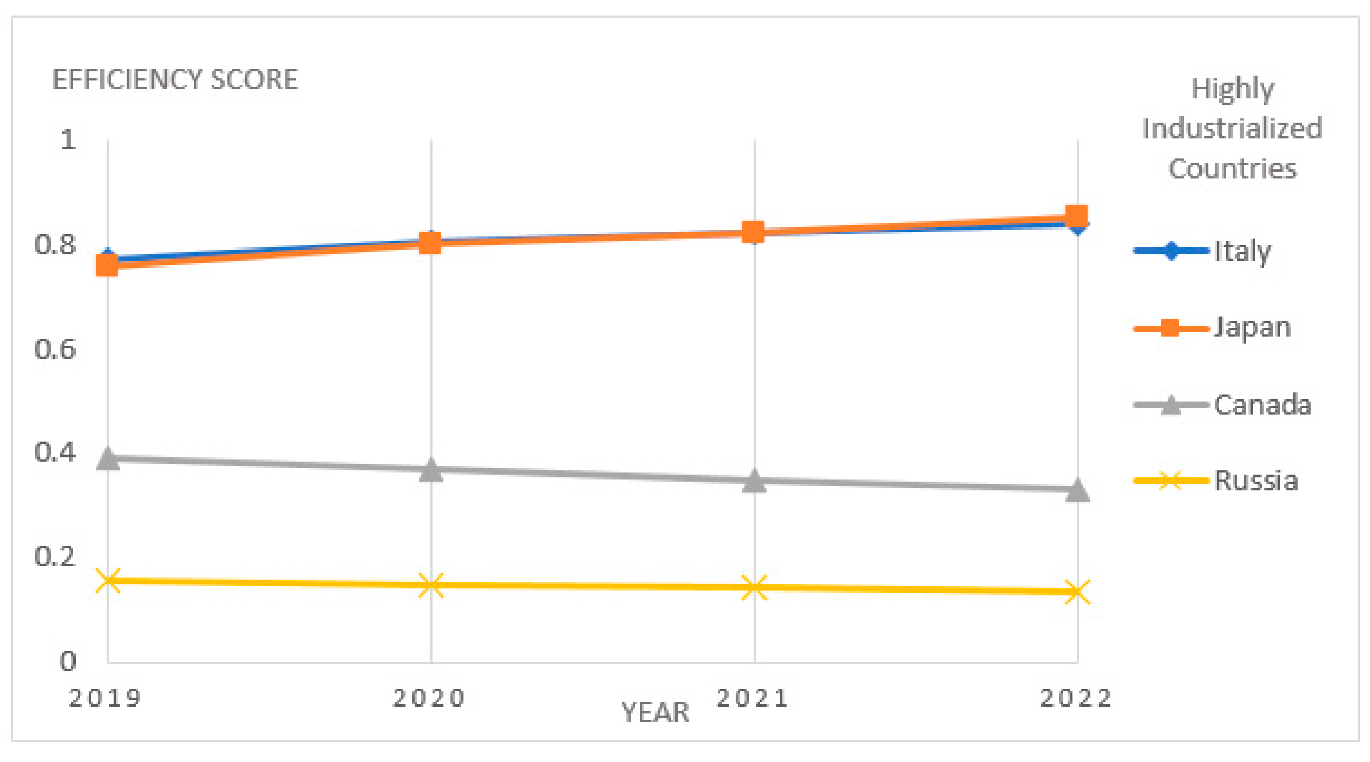
Figure 5 does not include the countries that obtain an efficiency score of 1 through the whole period of 2019 to 2022 as they are understood to be highly efficient already. It can be observed that Italy and Japan display a quite positive trend, with a slight increase in efficiency, while Canada and Russia have a slightly negative trend.
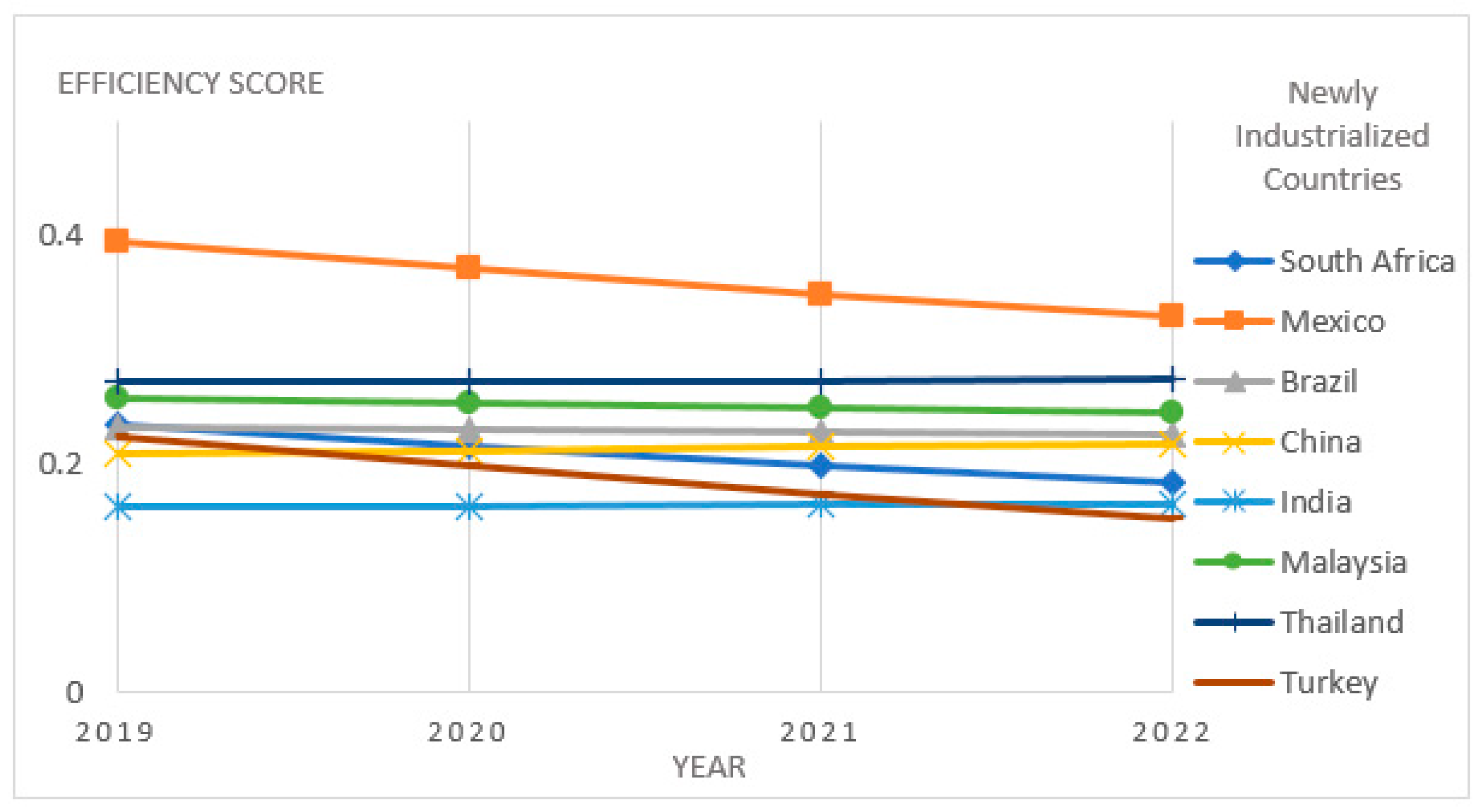
Efficiency scores of the NICs are mostly around of below a 0.5 level, except for Indonesia which garnered a score of 1.0 from 2019 to 2022. None of the countries show any remarkable positive trends. Instead, some countries like China, India, and Thailand are expected to display stable performance or very little improvement in efficiency. Mexico, Thailand, and Turkey will have declining efficiencies during the projected period, as seen in Figure 6.
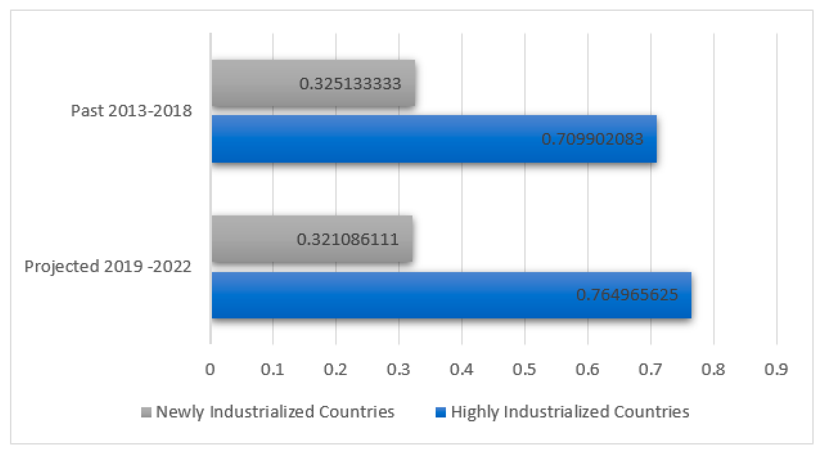
As presented in Figure 7, the calculated average efficiencies of HICs during the past and projected periods are comparatively higher than the NICs. However due to the existence of the very low efficiency scores of Russia and Canada, the effect to the average efficiency scores of the HIC group reached the 0.7099 level for the past period and is expected to increase by 7.76% to reach the 0.765 projected efficiency level. A different scenario is expected from the NIC group which will exhibit a decline of 1.23% from a 0.325 score down to a projected average level of 0.321.

5. Conclusions

With the implementation of the Paris Agreement signed by the HICs and NICs, the results show different effects on each country. Some countries have efficiently utilized their renewable energy resources, but some are not doing so, while others have maintained their levels and it seems they are not moved by the Agreement terms. The use of the undesirable model has successfully calculated each country’s position in terms of the utilization of their resources while considering greatly a very bad factor, which is the carbon emission.
Knowing the economic capabilities of the highly industrialized nations, the results show that Russia is the least efficient among them. A mean efficiency score of 0.1801 verifies the country’s lack of attention to its renewable energy program. In fact, in 2015, renewable energy only comprised 20% of the total installed power capacity, which mostly came from bioenergy and hydropower. The country must focus on other sources such as geothermal, wind, and solar photovoltaic (PV) [42]. Canada, with a mean efficiency score of 0.4221 manages to place second to the last among the HICs. A report from 2015 reveals that Vancouver alone sourced its 69% of energy from fossil fuels and 31% from renewable sources [43]. The situation in Japan is a little different, as due to the nuclear disaster from a major earthquake years ago, the country aims their energy to be completely 100% supplied by renewable energy, especially in their local regions, by 2020 [44]. Additionally, a report states that there is a decrease in the use of fossil fuels in 2018, 78% from 81% share. However, a dependency of the country on nuclear energy still exists and is evident from the increase of its generation from 2.8% to 4.7% of the same year [45]. This can be one of the reasons for Japan’s efficiency score drop from 2016 to 2018 and its acquisition of an average of 0.6671 throughout the studied period. The same goal is seen in Italy’s energy program. With the introduction of the 20-20-20 EU goals, the Italian government aims to decrease the emission of greenhouse gases by 20%, improve energy savings to up to 20%, and attain a 20% generation of renewable energy by 2020 [46]. The result of this study shows that Italy has quite improved its renewable energy utilization with increased and maintained efficiency scores from 2015 to 2018. While reaching a perfect efficiency of 1.0 in 2018, the average score becomes 0.7108 due to lower scores acquired from previous years. These scores imply that the German government has effectively improved its renewable energy utilization throughout the study period. Gaining an efficiency score of 1.0 throughout the study period, France, the United Kingdom, and United States, have been consistently utilized their renewable energies even before or after the Paris agreement. Their energy and sustainability programs can be a benchmark for other HICs that aim to improve their use of own renewable resources.
In contrast with the efficiency scores of the HICs, none from the list of NICs is able to get a consistent perfect efficiency. In spite of this, Indonesia manages to acquire perfect efficiency during the period of 2015 to 2018 rising from low-efficiency scores. Getting the highest mean efficiency score of 0.7645 among the NICs, this can be due to the fact that the country is considered to have the biggest resources of geothermal energy in the world [47]. South Africa demonstrates an interesting efficiency score as it can be seen that during the period of 2013 to 2014, the country was able to gain a perfect efficiency. This performance is attributable to their noticeable increase in renewable energy production in previous years [48]. However, this performance by South Africa was not maintained since the country’s efficiency dropped tremendously in succeeding years resulting in an average efficiency score of only 0.5185. Mexico, Turkey, Brazil, Malaysia, and Thailand are performing consistently at a low-level efficiency, with a minimum of 0.2278 and a maximum of 0.2734 mean scores. These results can be caused by the following factors: Mexico’s dependency on fossil fuels wherein 85% of their total power was produced in 2012 [49]; Turkey’s power sector industry as the biggest contributor to CO2 emissions and a high reliance to coal-powered electricity generation accounting to 37.2% of their total electricity [50]; the old structure of Brazil’s energy sector which limits their capacities in handling renewable energy demands, and other political factors that hinder the country’s development to successfully execute their national energy programs [51]; and, Malaysia and Thailand’s high proportional use of crude oil, coal, and natural gas, giving less importance to renewable energies [52,53].
The HIC group is expected to keep increasing the efficiency level by 7.76% from the past period to the projected period. This can be due to the expected development to the future renewable energy developments by Japan and Italy. However, the NIC group is expected a bit decline in the average efficiency with negative 1.23% due to the efficiency drop performance by Turkey and Mexico along with the low efficiency performances by other countries.
Future implications from the result of combined data gathered using grey prediction and the undesirable DEA model shows that the HICs and NICs will continuously follow the trend of the efficiency scores for all these countries with Germany joining the group of perfectly efficient ones together with Indonesia, France, United Kingdom, and the United States. All other HICs and NICs will perform otherwise, especially if they will not concede significant importance to renewable energy. Most of the developments in the use of the renewable energy begin with the improvement in the political and legal structure surrounding its use and regulation, providing incentives or tax exemptions to private power producers to shift in using the renewable energy. Countries can also build strong partnerships with non-government and international organizations that are focusing on providing assistance to countries that want to achieve sustainable and renewable energy production. Strengthening the support to the research and development sector to determine the suitable sites to deploy renewable energy sources such as solar, wind and wave energy. Long-term strategic plans for renewable energy development that will also consider the economic, social, and environmental impacts to the country.
This study contributes as a method to mathematically evaluate the energy utilization efficiency of HICs and NICs based on available public data. The DEA undesirable model treatment of the CO2 emission factor as a less important factor made this study different from the others. Hence, this model is the most appropriate method to evaluate the energy sector that uses data with undesired factors. The results of this research may guide each country for improvement of its production and consumption towards sustainable renewable energy development. This can also help policymakers, government agencies and the energy sectors to address the problem in the existence of bad outputs such as CO2 emissions. For future studies involving quantitative measurements, the authors recommend combining DEA with a qualitative evaluation approach such as the one described in Wang et al. [54], which uses the fuzzy analytical hierarchy process for analysis to improve studies of this kind.

Author Contributions

Conceptualization, C.-N.W. and H.T.; data curation, H.T. and D.H.D.; formal analysis, H.T. and D.H.D.; funding acquisition, C.-N.W.; investigation, H.T. and D.H.D.; methodology, C.-N.W., H.T., and D.H.D.; project administration, C.-N.W.; writing—original draft, H.T. and D.H.D.; writing—review and editing, C.-N.W. and H.T. All authors have read and agreed to the published version of the manuscript.

Funding

This research was partly supported by National Kaohsiung University of Science and Technology, and project number 108-2622-E-992-017-CC3 from the Ministry of Sciences and Technology in Taiwan.

Acknowledgments

The authors appreciate the support from Taiwan National Kaohsiung University of Science and Technology, Philippines Technological University of the Philippines Taguig, and Taiwan Ministry of Sciences and Technology.

Conflicts of Interest

The authors declare no conflict of interest.

References

  1. United Nations. Adoption of the Paris Agreement. In Proceedings of the Conference of the Parties, Paris, France, 30 November–11 December 2015. [Google Scholar]
  2. Nejat, P.; Jomehzadeh, F.; Taheri, M.M.; Gohari, M.; Majid, M.Z.A. A global review of energy consumption, CO2 emissions and policy in the residential sector (with an overview of the top ten CO2 emitting countries). Renew. Sustain. Energy Rev. 2015, 43, 843–862. [Google Scholar] [CrossRef]
  3. Ellabban, O.; Abu-Rub, H.; Blaabjerg, F. Renewable energy resources: Current status, future prospects and their enabling technology. Renew. Sustain. Energy Rev. 2014, 39, 748–764. [Google Scholar] [CrossRef]
  4. The International Renewable Energy Agency (IRENA). Available online: https://www.irena.org/aboutirena (accessed on 4 December 2019).
  5. Laub, Z. The Group of Eight (G8) Industrialized Nations. Counsil on Foreign Relations. 2014. Available online: http://www.cfr.org/backgrounder/group-eight-g8-industrialized-nations/ (accessed on 6 December 2019).
  6. Szirmai, A.; Naudé, W.; Alcorta, L. Pathways to Industrialization in the Twenty-First Century: New Challenges and Emerging Paradigms; OUP Oxford: Oxford, UK, 2013. [Google Scholar]
  7. Cleveland, C.J.; Kaufmann, R.K.; Stern, D.I. Aggregation and the role of energy in the economy. Ecol. Econ. 2000, 32, 301–317. [Google Scholar] [CrossRef]
  8. Cîrstea, S.D.; Moldovan-Teselios, C.; Cîrstea, A.; Turcu, A.C.; Darab, C.P. Evaluating renewable energy sustainability by composite index. Sustainability 2018, 10, 811. [Google Scholar] [CrossRef] [Green Version]
  9. Iddrisu, I.; Bhattacharyya, S.C. Sustainable Energy Development Index: A multi-dimensional indicator for measuring sustainable energy development. Renew. Sustain. Energy Rev. 2015, 50, 513–530. [Google Scholar] [CrossRef] [Green Version]
  10. Lee, C.W.; Zhong, J. Construction of a responsible investment composite index for renewable energy industry. Renew. Sustain. Energy Rev. 2015, 51, 288–303. [Google Scholar] [CrossRef]
  11. Schlör, H.; Fischer, W.; Hake, J.-F. Methods of measuring sustainable development of the German energy sector. Appl. Energy 2013, 101, 172–181. [Google Scholar] [CrossRef]
  12. Liu, G. Development of a general sustainability indicator for renewable energy systems: A review. Renew. Sustain. Energy Rev. 2014, 31, 611–621. [Google Scholar] [CrossRef]
  13. Doukas, H.; Papadopoulou, A.; Savvakis, N.; Tsoutsos, T.; Psarras, J. Assessing energy sustainability of rural communities using Principal Component Analysis. Renew. Sustain. Energy Rev. 2012, 16, 1949–1957. [Google Scholar] [CrossRef]
  14. Štreimikienė, D.; Šliogerienė, J.; Turskis, Z. Multi-criteria analysis of electricity generation technologies in Lithuania. Renew. Energy 2016, 85, 148–156. [Google Scholar] [CrossRef]
  15. Ren, J.; Sovacool, B.K. Prioritizing low-carbon energy sources to enhance China’s energy security. Energy Convers. Manag. 2015, 92, 129–136. [Google Scholar] [CrossRef]
  16. Troldborg, M.; Heslop, S.; Hough, R.L. Assessing the sustainability of renewable energy technologies using multi-criteria analysis: Suitability of approach for national-scale assessments and associated uncertainties. Renew. Sustain. Energy Rev. 2014, 39, 1173–1184. [Google Scholar] [CrossRef]
  17. Yazdani-Chamzini, A.; Fouladgar, M.M.; Zavadskas, E.K.; Moini, S.H.H. Selecting the optimal renewable energy using multi criteria decision making. J. Bus. Econ. Manag. 2013, 14, 957–978. [Google Scholar] [CrossRef]
  18. San Cristóbal, J. Multi-criteria decision-making in the selection of a renewable energy project in spain: The Vikor method. Renew. Energy 2011, 36, 498–502. [Google Scholar] [CrossRef]
  19. Kabak, M.; Dağdeviren, M. Prioritization of renewable energy sources for Turkey by using a hybrid MCDM methodology. Energy Convers. Manag. 2014, 79, 25–33. [Google Scholar] [CrossRef]
  20. Halkos, G.E.; Tzeremes, N.G. Measuring the effect of Kyoto protocol agreement on countries’ environmental efficiency in CO2 emissions: An application of conditional full frontiers. J. Prod. Anal. 2014, 41, 367–382. [Google Scholar] [CrossRef] [Green Version]
  21. Wang, C.-N.; Ho, H.-X.T.; Luo, S.-H.; Lin, T.-F. An integrated approach to evaluating and selecting green logistics providers for sustainable development. Sustainability 2017, 9, 218. [Google Scholar] [CrossRef] [Green Version]
  22. Oggioni, G.; Riccardi, R.; Toninelli, R. Eco-efficiency of the world cement industry: A data envelopment analysis. Energy Policy 2011, 39, 2842–2854. [Google Scholar] [CrossRef]
  23. Woo, C.; Chung, Y.; Chun, D.; Seo, H.; Hong, S. The static and dynamic environmental efficiency of renewable energy: A Malmquist index analysis of OECD countries. Renew. Sustain. Energy Rev. 2015, 47, 367–376. [Google Scholar] [CrossRef]
  24. Zhou, P.; Ang, B.; Han, J. Total factor carbon emission performance: A Malmquist index analysis. Energy Econ. 2010, 32, 194–201. [Google Scholar] [CrossRef]
  25. Wang, C.-N.; Nguyen, T.-D.; Yu, M.-C. Energy Use Efficiency Past-to-Future Evaluation: An International Comparison. Energies 2019, 12, 3804. [Google Scholar] [CrossRef] [Green Version]
  26. Zofío, J.L.; Prieto, A.M. Environmental efficiency and regulatory standards: The case of CO2 emissions from OECD industries. Resour. Energy Econ. 2001, 23, 63–83. [Google Scholar] [CrossRef]
  27. Xie, B.-C.; Shang, L.-F.; Yang, S.-B.; Yi, B.-W. Dynamic environmental efficiency evaluation of electric power industries: Evidence from OECD (Organization for Economic Cooperation and Development) and BRIC (Brazil, Russia, India and China) countries. Energy 2014, 74, 147–157. [Google Scholar] [CrossRef]
  28. Cicea, C.; Marinescu, C.; Popa, I.; Dobrin, C. Environmental efficiency of investments in renewable energy: Comparative analysis at macroeconomic level. Renew. Sustain. Energy Rev. 2014, 30, 555–564. [Google Scholar] [CrossRef]
  29. Wang, C.-N.; Luu, Q.-C.; Nguyen, T.-K.-L. Estimating Relative Efficiency of Electricity Consumption in 42 Countries during the Period of 2008–2017. Energies 2018, 11, 3037. [Google Scholar] [CrossRef] [Green Version]
  30. Chien, T.; Hu, J.-L. Renewable energy and macroeconomic efficiency of OECD and non-OECD economies. Energy Policy 2007, 35, 3606–3615. [Google Scholar] [CrossRef]
  31. Charnes, A.; Cooper, W.W.; Rhodes, E. Measuring the efficiency of decision making units. Eur. J. Operat. Res. 1978, 2, 429–444. [Google Scholar] [CrossRef]
  32. Banker, R.D.; Charnes, A.; Cooper, W.W. Some models for estimating technical and scale inefficiencies in data envelopment analysis. Manag. Sci. 1984, 30, 1078–1092. [Google Scholar] [CrossRef] [Green Version]
  33. Caves, D.W.; Christensen, L.R.; Diewert, W.E. The economic theory of index numbers and the measurement of input, output, and productivity. Econ. J. Econ. Soc. 1982, 50, 1393–1414. [Google Scholar] [CrossRef]
  34. Färe, R.; Grosskopf, S.; Lindgren, B.; Roos, P. Productivity changes in Swedish pharamacies 1980–1989: A non-parametric Malmquist approach. J. Prod. Anal. 1992, 3, 85–101. [Google Scholar] [CrossRef]
  35. Ahn, T.; Charnes, A.; Cooper, W.W. Some statistical and DEA evaluations of relative efficiencies of public and private institutions of higher learning. Socio-Econ. Plan. Sci. 1988, 22, 259–269. [Google Scholar] [CrossRef]
  36. Tone, K. A slacks-based measure of efficiency in data envelopment analysis. Eur. J. Operat. Res. 2001, 130, 498–509. [Google Scholar] [CrossRef] [Green Version]
  37. Cooper, W.W.; Seiford, L.M.; Tone, K. Introduction to Data Envelopment Analysis and its Uses: With DEA-Solver Software and References; Springer Science & Business Media: New York, NY, USA, 2006. [Google Scholar]
  38. Wang, C.-N.; Nguyen, T.-D.; Le, M.-D. Assessing Performance Efficiency of Information and Communication Technology Industry-Forecasting and Evaluating: The Case in Vietnam. Appl. Sci. 2019, 9, 3996. [Google Scholar] [CrossRef] [Green Version]
  39. Julong, D. Introduction to grey system theory. J. Grey Syst. 1989, 1, 1–24. [Google Scholar]
  40. Tseng, F.-M.; Yu, H.-C.; Tzeng, G.-H. Applied hybrid grey model to forecast seasonal time series. Technol. Forecast. Soc. Chang. 2001, 67, 291–302. [Google Scholar] [CrossRef]
  41. Ju-Long, D. Control problems of grey systems. Syst. Control Lett. 1982, 1, 288–294. [Google Scholar] [CrossRef]
  42. Gielen, D.; Saygin, D. REmap 2030 Renewable Energy Prospects for Russian Federation. Abu Dhabi. 2017. Available online: http://www.irena.org/remap (accessed on 6 April 2020).
  43. Ahmed, S.; Pourya, S.; Michael, W.; Doug, S.; Jinlei, F.; Ghislaine, K.; Verena, O.; Michael, R. Adopting and Promoting a 100% Renewable Energy Target; International Renewable Energy Agency: Vancouver, BC, Canada, 2018. [Google Scholar]
  44. Esteban, M.; Portugal-Pereira, J. Post-disaster resilience of a 100% renewable energy system in Japan. Energy 2014, 68, 756–764. [Google Scholar] [CrossRef]
  45. Share of Renewable Energy Power in Japan, 2018 (Preliminary Report); Institute for Sustainable Energy Policies: Tokyo, Japan, 2019.
  46. Antonelli, M.; Desideri, U.; Franco, A. Effects of large scale penetration of renewables: The Italian case in the years 2008–2015. Renew. Sustain. Energy Rev. 2018, 81, 3090–3100. [Google Scholar] [CrossRef]
  47. Winarno, O.T.; Alwendra, Y.; Mujiyanto, S. Policies and strategies for renewable energy development in Indonesia. In Proceedings of the 2016 IEEE International Conference on Renewable Energy Research and Applications (ICRERA), Birmingham, UK, 20–23 November 2016; pp. 270–272. [Google Scholar]
  48. Nakumuryango, A.; Inglesi-Lotz, R. South Africa’s performance on renewable energy and its relative position against the OECD countries and the rest of Africa. Renew. Sustain. Energy Rev. 2016, 56, 999–1007. [Google Scholar] [CrossRef] [Green Version]
  49. Vidal-Amaro, J.J.; Østergaard, P.A.; Sheinbaum-Pardo, C. Optimal energy mix for transitioning from fossil fuels to renewable energy sources—The case of the Mexican electricity system. Appl. Energy 2015, 150, 80–96. [Google Scholar] [CrossRef]
  50. Karagöz, G.N. Renewable Energy in Turkey: A Cleaner, Self-Sufficient Alternative to Coal; Kadir Has Üniversitesi: Istanbul, Turkey, 2019. [Google Scholar]
  51. de Melo, C.A.; de Martino Jannuzzi, G.; Bajay, S.V. Nonconventional renewable energy governance in Brazil: Lessons to learn from the German experience. Renew. Sustain. Energy Rev. 2016, 61, 222–234. [Google Scholar] [CrossRef]
  52. Khor, C.S.; Lalchand, G. A review on sustainable power generation in Malaysia to 2030: Historical perspective, current assessment, and future strategies. Renew. Sustain. Energy Rev. 2014, 29, 952–960. [Google Scholar] [CrossRef]
  53. Kumar, S. Assessment of renewables for energy security and carbon mitigation in Southeast Asia: The case of Indonesia and Thailand. Appl. Energy 2016, 163, 63–70. [Google Scholar] [CrossRef]
  54. Wang, C.-N.; Nguyen, V.T.; Thai, H.T.N.; Tran, N.N.; Tran, T.L.A. Sustainable supplier selection process in edible oil production by a hybrid fuzzy analytical hierarchy process and green data envelopment analysis for the SMEs food processing industry. Mathematics 2018, 6, 302. [Google Scholar] [CrossRef] [Green Version]
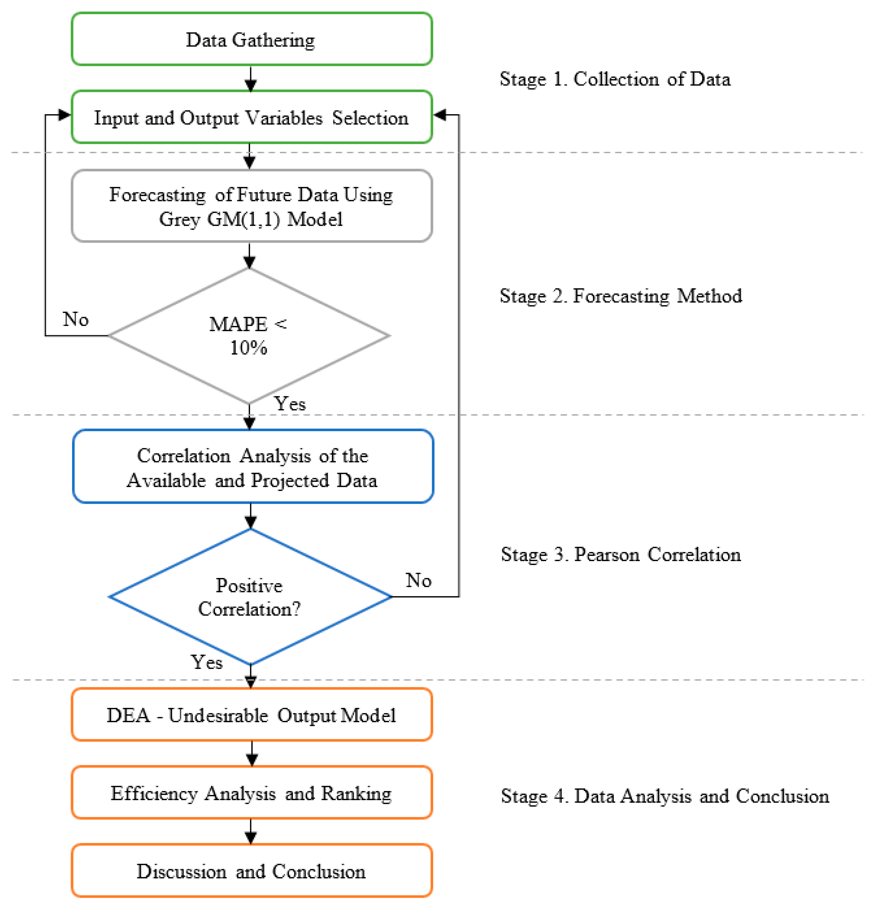
Figure 1. The research process.
Energies 13 02629 g001
Figure 2. The grey prediction model procedure.
Energies 13 02629 g002
Figure 3. Graphical Presentation of other HICs Efficiency Scores (<1.0) from 2013–2018.
Energies 13 02629 g003
Figure 4. Graphical Presentation NICs Efficiency Scores (<1.0) from 2013–2018.
Energies 13 02629 g004
Figure 5. Graphical Presentation of other HICs’ Efficiency Scores (<1.0) from 2019–2022.
Energies 13 02629 g005
Figure 6. Graphical Presentation of NICs’ Efficiency Scores from 2019–2022.
Energies 13 02629 g006
Figure 7. Comparative graph of HICs and NICs average efficiency scores for two different periods.
Energies 13 02629 g007
Table 1. List of commonly used input and output factors for several past literature.
Authors,
Year [References]
FactorsMethod/sNo. of Counties
InputsOutputs
Zofio and Prieto, 2001
[26]
Energy Consumption
Capital stock
Labor
GDP
CO2 emission
DEA18
Xie et al., 2014 [27]Labor
Installed capacity
Fuel and nuclear
Power generation
CO2 emission
DEA-SBM26
Cicea et al., 2014 [28]GDP capita
Energy intensity
Investment to renewables
CO2 emissionDEA22
Wang et al., 2018 [29]Energy Consumption
Population
GDP
CO2
CH4 methane
N2O nitrous oxide
DEA-Undesirable model42
Chien and Hu, 2009 [30]Capital stock
Energy consumption
Labor
GDPDEA45
Table 2. Equivalent forecast category for every MAPE percentage score.
MAPEForecast Categories
<10%High Accuracy
10–20%Good
20–50%Reasonable
>50%Inaccurate
Table 3. Name of the countries in their respective DMU number and group.
DMU No.Highly Industrialized Countries (HIC)DMU No.Newly Industrialized Countries (NIC)
CTRY1FranceCTRY9South Africa
CTRY2GermanyCTRY10Mexico
CTRY3ItalyCTRY11Brazil
CTRY4United KingdomCTRY12China
CTRY5JapanCTRY13India
CTRY6United StatesCTRY14Indonesia
CTRY7CanadaCTRY15Malaysia
CTRY8RussiaCTRY16Thailand
CTRY17Turkey
Table 4. Descriptive statistics and Pearson correlation coefficients of the year 2015.
Input FactorsOutput Factors
Total Renewable Energy Capacity in GW (TREC)Labor Force
In millions (LF)
Total Energy Consumption in Mtoe (TEC)Carbon Dioxide Emission in MtCO2 (CO2)Gross Domestic Product in $ Million (GDP)
Descriptive Statistics
Max479.11785,372.422993.909061.2618,219.3
Min3.4314,589.3586.33228.53296.64
Average80.98124,337.42560.541401.993229.5
SD110.48197,968.12780.222226.364468.96
Correlation Scores
TREC10.82740.91910.94670.7080
LF0.827410.81040.85150.4637
TEC0.91910.810410.98880.8581
CO20.94670.85150.988810.7941
GDP0.70800.46370.85810.79411
Note: The scores of the correlation coefficient are all positive values from 2013–2018. 2015 data is used to represent the other year periods.
Table 5. Summary of the average mean absolute percentage error (MAPE) of HICs and NICs.
DMU No.CountryTRECLFTECCO2GDPAverage
CTRY1France0.21%0.09%0.39%1.02%4.81%1.30%
CTRY2Germany0.34%0.20%0.85%0.99%4.60%1.39%
CTRY3Italy0.37%0.25%0.59%0.71%4.65%1.31%
CTRY4United Kingdom2.85%0.06%0.32%0.72%3.03%1.40%
CTRY5Japan2.28%0.19%0.35%0.44%2.51%1.15%
CTRY6United States0.77%0.14%1.00%1.37%0.46%0.75%
CTRY7Canada1.24%0.14%0.80%0.63%4.57%1.48%
CTRY8Russia0.13%0.21%1.42%1.29%12.82%3.17%
CTRY9South Africa5.17%0.43%1.14%1.38%5.29%2.68%
CTRY10Mexico1.51%0.09%0.62%1.39%4.51%1.62%
CTRY11Brazil0.31%0.14%0.89%1.26%8.10%2.14%
CTRY12China0.52%0.07%0.94%0.83%2.12%0.90%
CTRY13India1.06%0.08%0.47%1.07%2.14%0.96%
CTRY14Indonesia0.40%0.28%0.96%1.49%2.01%1.03%
CTRY15Malaysia3.33%0.08%1.21%0.53%5.40%2.11%
CTRY16Thailand1.96%0.17%0.34%0.55%2.84%1.17%
Source: Calculated by the authors.
Table 6. Descriptive statistics and Pearson correlation coefficients using the projected values for the year 2021.
Input FactorsOutput Factors
Total Renewable Energy Capacity in GW (TREC)Labor Force
In millions (LF)
Total Energy Consumption in Mtoe (TEC)Carbon Dioxide Emission in MtCO2 (CO2)Gross Domestic Product in $ Million (GDP)
Descriptive Statistics
Max1025.678788,934.323265.259,616.3422,840.18
Min9.7916,459.7094.97240.41347.94
Average142.74130,441.84604.621475.283965.78
SD233.78203,616.31839.582342.195920.01
Correlation Scores
TREC10.85310.91100.95120.7194
LF0.853110.82120.85970.5379
TEC0.91100.821210.98880.8774
CO20.95120.85970.988810.8226
GDP0.71940.53790.87740.82261
Note: The scores of the correlation coefficient are all positive values from 2019–2022. The data from 2021 is used to represent the other year periods.
Table 7. Efficiency scores of countries and group rankings from period from 2013 to 2018.
CountriesYear Periods and Rankings
2013Rank2014Rank2015Rank2016Rank2017Rank2018Rank
Highly Industrialized Countries (HICs)
CTRY11.000011.000011.000011.000011.000011.00001
CTRY20.703060.627750.551860.649860.732651.00001
CTRY30.778340.682940.586040.679450.735840.73255
CTRY41.000011.000011.000011.000011.000011.00001
CTRY50.734150.592860.564750.718740.715360.67706
CTRY61.000011.000011.000011.000011.000011.00001
CTRY70.511770.411570.364870.394570.434170.41577
CTRY80.221580.188780.141780.153180.185280.19048
Newly Industrialized Countries (NICs)
CTRY91.000011.000010.300030.260040.276040.27484
CTRY100.357420.343920.345520.351820.402020.38732
CTRY110.336240.271850.205060.233850.279130.22666
CTRY120.133880.131580.150080.166880.181180.18408
CTRY130.100190.099390.115090.135190.153790.14119
CTRY140.299350.287731.000011.000011.000011.00001
CTRY150.228560.218560.204970.230960.256870.28103
CTRY160.205570.187670.210450.229170.262660.27165
CTRY170.336330.279340.263440.280630.265350.21527
Source: Calculated by the authors.
Table 8. Average Efficiency Scores and Overall Rankings of HICs and NICs.
DMU No.CountriesAverage Efficiency ScoreOverall Ranking
Highly Industrialized Countries
CTRY1France1.00001
CTRY4United Kingdom1.00001
CTRY6United States1.00001
CTRY2Germany0.71084
sCTRY3Italy0.69925
CTRY5Japan0.66716
CTRY7Canada0.42217
CTRY8Russia0.18018
Newly Industrialized Countries
CTRY14Indonesia0.76451
CTRY9South Africa0.51852
CTRY10Mexico0.36473
CTRY17Turkey0.27344
CTRY11Brazil0.25885
CTRY15Malaysia0.23686
CTRY16Thailand0.22787
CTRY12China0.15798
CTRY13India0.12419
Source: Calculated by the authors.
Table 9. Projected efficiency scores of countries and group rankings from period from 2019 to 2022.
CountriesYear Periods and Rankings
2019Rank2020Rank2021Rank2022Rank
Highly Industrialized Countries (HICs)
CTRY11.000011.000011.000011.00001
CTRY21.000011.000011.000011.00001
CTRY30.768750.803050.820850.83816
CTRY41.000011.000011.000011.00001
CTRY50.757760.797760.820760.84935
CTRY61.000011.000011.000011.00001
CTRY70.390970.368670.348270.32957
CTRY80.158080.149880.142380.13568
Newly Industrialized Countries (NICs)
CTRY90.234250.215260.198370.18347
CTRY100.395820.371720.349520.32882
CTRY110.233260.230850.228650.22615
CTRY120.210180.212670.214960.21736
CTRY130.162790.163990.165190.16648
CTRY141.000011.000011.000011.00001
CTRY150.257640.253240.248940.24474
CTRY160.272030.272830.273730.27473
CTRY170.224870.199980.174880.15349
Source: Calculated by the authors.