The Influence of an Additional Sensor on the Microprocessor Temperature


1
Department of Electronics and Information Systems, University of Ghent, Technologiepark Zwijnaarde 126, 9052 Zwijnaarde, Belgium
2
Institute of Electronics, AGH University of Science and Technology, Al. Mickiewicza 30, 30-059 Cracow, Poland
*
Author to whom correspondence should be addressed.
Energies 2020, 13(12), 3156; https://doi.org/10.3390/en13123156
Submission received: 12 May 2020
/
Revised: 10 June 2020
/
Accepted: 17 June 2020
/
Published: 18 June 2020
(This article belongs to the Special Issue Latest Advances in Electrothermal Models)
Abstract
:This paper deals with the problem of inserting a temperature sensor in the neighbourhood of a chip to monitor the junction temperature. If the sensor is not in the middle of the heat source, the recorded temperature can be quite different from the chip temperature we are mainly interested in. For the steady state temperature, it is rather easy to introduce a correction factor. For the transient behaviour of the temperature, there is a tremendous difference between the chip and the sensor temperature, which cannot be neglected if the temperature is used as a parameter to change, for example, the clock frequency in order to improve the throughput.
1. Introduction
Thermal management is a crucial issue in high speed data processing today. The problem has been attacked by many authors, e.g., they propose three techniques to create sensor infrastructures for monitoring the maximum temperature of a multicore system [1]. In [2], the systematic techniques for determining the optimal locations for thermal sensors to provide high-fidelity thermal monitoring of a complex microprocessor system are presented. Another paper presents a compact thermal model that can be integrated with modern Computer Aided Design tools to achieve a temperature-aware design methodology [3].
Data processing with the use of electron devices involves heat losses, which hamper the speed of the processing. Some kinds of cooling systems are used; however, some of them consume additional energy, make noise and enlarge the dimensions of mobile devices. In previously published papers, the authors presented a new idea: one additional temperature sensor, placed on the heat sink. Measuring the temperature difference between the processor and heat sink yields valuable information, which is able to improve the microprocessor’s throughput without any changes in its design [4,5]. The theoretical research of these articles was supplemented with experiments using a portable computer: MSI U270 (Micro-Star International Co., Ltd).
It must also be stressed that in this paper, we are dealing with transient or time-dependent thermal problems. Some time ago, there was only interest in steady-state temperatures. Data books only provided thermal resistance. For the power consumption, only a Direct Current (DC) value was given. Recently, more and more attention is paid to transient analyses [6,7,8,9,10,11,12]. From these measurements, one can set up equivalent Foster and Cauer Resistor-Capacitor (RC) networks, also known as structure functions [13]. The time constant distribution has also been proved to give a lot of useful information about the thermal path between the chip and the ambient temperature [14]. Just like for linear electric circuit analysis, the time-dependent analysis was mainly done in the AC domain. It turned out that for thermal problems, the Alternating Current (AC) approach was very useful. These studies have been applied to electronic packages [15,16,17,18], cooling fins [19,20], underground and overhead high voltage cables [21,22,23,24], integrated inductors [25], heat pipes [26] and photovoltaic panels [27].
The title of this paper clearly mentions “additional temperature sensor”. Usually, an integrated circuit is fully designed and, at the last minute, the idea is put forward to include some temperature monitoring. In order to avoid a completely new design, the decision is then made to put the temperature sensor “aside” or in a free place, if available. This creates a particular problem that will be discussed in this paper.
2. Experimental Measurements
Measurements have been carried out on a Samsung RC dual core, including AMD E-350 (AMD, USA). This chip contains a dual core GPU Radeon 6320/6310 C (ATI Technologies, Markham, ON, Canada). Figure 1 shows the activity (or CPU usage) and the temperature of the CPU versus time. The temperature of the GPU is also displayed. The GPU is a different integrated circuit. The chip contains a dual core CPU (2x Bobcat) with a L2 Cache (L2 Cache—it is a level of memory, general meaning), a GPU with DirectX v11 GFX (Microsoft), and RAM DDR3 (standard); its temperature will not be used further on in our analysis. Nevertheless, it is clear that both temperatures have a similar, almost identical behaviour. Note that all the temperatures are temperature rises above ambient temperature, i.e., of the metal base plate connected to the cooling fin through a heat pipe.
Special software has been installed to measure the activity of the CPU. Activity is measured on a relative scale from 0 to 100. Figure 1 clearly demonstrates the correlation between the activity and the CPU temperature. During the first 21.6 min (=arrow shown in Figure 1), the activity varies around the value of 20. After that period, the activity was increased by a factor 4.5 up to a value around 90. Nevertheless, the temperature rises from 59° to 88° (=59° + 29°) (after extrapolation to steady state). Hence, the temperature is not proportional to the activity. This is due to the technology used for the processor. The power dissipation (and hence the temperature rise) consists of two components: a constant value and a variable component proportional to the clock frequency or, in other words, the activity.
3. Network Model
As shown in Figure 2, the experimental recorded CPU temperature (Figure 1) can be quite well fitted to the following function:
The moment t = 0 in Figure 2 is taken as the starting point of the increased activity of the CPU. It corresponds to the moment around 21.6 min (arrow in Figure 1). Note that the Function (1) satisfies the initial conditions T = 58° and dT/dt = 0 at the moment t = 0. The temperature of 58° is the steady state temperature rise during the long reduced activity period (t < 0). For modelling, this constant value will no longer be taken into consideration, because we are mainly interested in the transient behaviour.
A closer look at Figure 1 reveals that the start of the increased activity can be approximately seen as a step function of the power consumption. It is then rather straightforward to establish an equivalent network giving rise to a transient temperature like Equation (1), provided a power step is inputted.
A quick look at Figure 1 shows there is a quite long delay between the start of the increased activity and the temperature rise. This proves that the temperature sensor is not in the middle of the heat source but at a certain distance, e.g., on edge of a heat sink. The heat has to propagate a certain time before any temperature rise can be recorded by the sensor. Figure 3 shows the proposed equivalent network. ΔP0 is the power step due to the increased activity. Note that the node S, where the temperature is evaluated, is not the input node CPU.
This is necessary to model the experimentally observed delay. The fact that the two exponential functions in Equation (1) have different signs also proves that we are dealing with transfer impedance. If the temperature would have been calculated at the input node, different signs, like in Equation (1), are physically impossible. Both the CPU and the sensor S are connected to the reference temperature through a thermal resistance R and a thermal capacitance C. We gave them both the same values because there are both within the same package. The coupling resistance R’ is responsible for the delay between the CPU and sensor’s temperature.
The sensor temperature ΔTS (Figure 3) is easily found to be given by:
where ΔP0 denotes the power step at the input. The method used to get Equation (2) is based on the use of symmetrical components as will be outlined in the appendix further on. In Equation (2), the time constants are given by:
The comparison between the experimental fitting, Equation (1), and the network solution, Equation (2), is quite straightforward. One may observe immediately that:
Although the CPU temperature is recorded at S, the displayed value has been multiplied by 2.81 in order to obtain the correct CPU temperature (at least during the steady state). This explains the values of almost 90° in Figure 1 during a high activity period. In order to obtain the correct sensor temperature, the expression (1) should be divided by 2.81.
In steady-state conditions, the total thermal resistance of the CPU to the base plate is the parallel connection of R and R’ + R:
According to the supplier’s information, a maximum temperature rise of 90° is obtained for a power dissipation between 45 and 50 Watts. Taking the average value 47.5 watts, we get:
From Equations (4) and (6), we get then the values of the resistor of the equivalent network.
From the knowledge on the thermal resistance R and the time constant τ1, one gets the value of the thermal capacitance C:
A thermal capacitance is, by definition, known as C = CvV, where cv is the specific heat per unit volume and V, the volume. Most solid materials have a volumetric specific heat of around 2 × 10⁶ J/m3K. Hence, we roughly get:
This seems to be a too high value at first sight. However, one should bear in mind that the chip is connected to the cooling fin through a heat pipe, which is a thermal short circuit. Hence, the volume of 43.8 cm3 is reasonable if one takes the heat pipe and the cooling fin into account.
4. Discussion
As already mentioned in the foregoing section, the sensor temperature differs from the CPU value that we are mainly interested in. A correction has been made, see Equation (5), so that the correct CPU temperature is obtained in steady-state conditions. However, we want to find out how much difference is obtained in case of a thermal transient problem.
To find an answer to that problem, one can use the equivalent network shown in Figure 3. If a step input power is applied, the sensor temperature ΔTS is given by Equation (2). The CPU temperature is then found to be:
Inserting the numerical values τ1 = 210 s, τ2 = 100 s and R′ = 1.818R in Equation (11), one gets:
Notice that in Equation (12), two minus signs appear, which is physically possible because we are dealing with an impedance function, i.e., the temperature is measured between the same nodes where the power is applied.
However, the curve ΔTS was multiplied by the correction factor 2.81 so that both curves have the same steady state value, so that a better comparison can be made. As can be seen from Figure 4, there is delay of about 100 s between the CPU and the temperature recorded by the sensor. As a consequence, a heat pulse lasting for less than 100 s will not be detected properly by the temperature sensor.
The curve ΔTCPU shows also a sharp rise at t = 0, which is typical for the temperature of a heat source. During the transient period, the sensor temperature gives a serious underestimate of the CPU temperature and, vice versa, an overestimation of the temperature will occur when the power is suddenly reduced.
It is also remarkable that a lot of information regarding the dynamic thermal properties could be gained from a graph like Figure 1. However, the processor was doing a job that has nothing to do with thermal analysis.
5. Conclusions
The investigation proves that if the temperatures are measured both inside the microprocessor structure and outside of it, e.g., at the cooling fin, the difference between the temperatures gives very useful information. It means that it is possible to increase the power dissipation in the mentioned periods of time without the temperature rising over assumed limit. As a consequence, the microprocessor’s throughput increases. Some examples carried out by the authors show that it is possible to improve the throughput even by 7% without any changes in the semiconductor structure, as has been published recently.
However, it has been clearly demonstrated in this paper that it is necessary to put the temperature-sensing device inside the heat source. As soon as the sensor is located at a certain distance, serious errors occur if one wants to measure the transient temperature behaviour. Regarding the steady-state temperature, a simple correction factor can be used, but for a transient problem, the inevitable delay cannot be adjusted by a simple correction factor.
Author Contributions
The conceptualization, formal analysis and methodology presented in this manuscript and their evaluation were carried out by all authors G.D.M. and A.K. The funding acquisition of the financial support for the project leading to this publication was made by A.K. All authors have read and agreed to the published version of the manuscript.
Funding
The research was supported financially from the AGH University of Science and Technology, Krakow, Poland subvention no. 16.16.230.434. The authors also want to express thanks to P. Fluder for his valuable contributions to the experimental measurements.
Conflicts of Interest
The authors declare no conflict of interest.
Appendix A
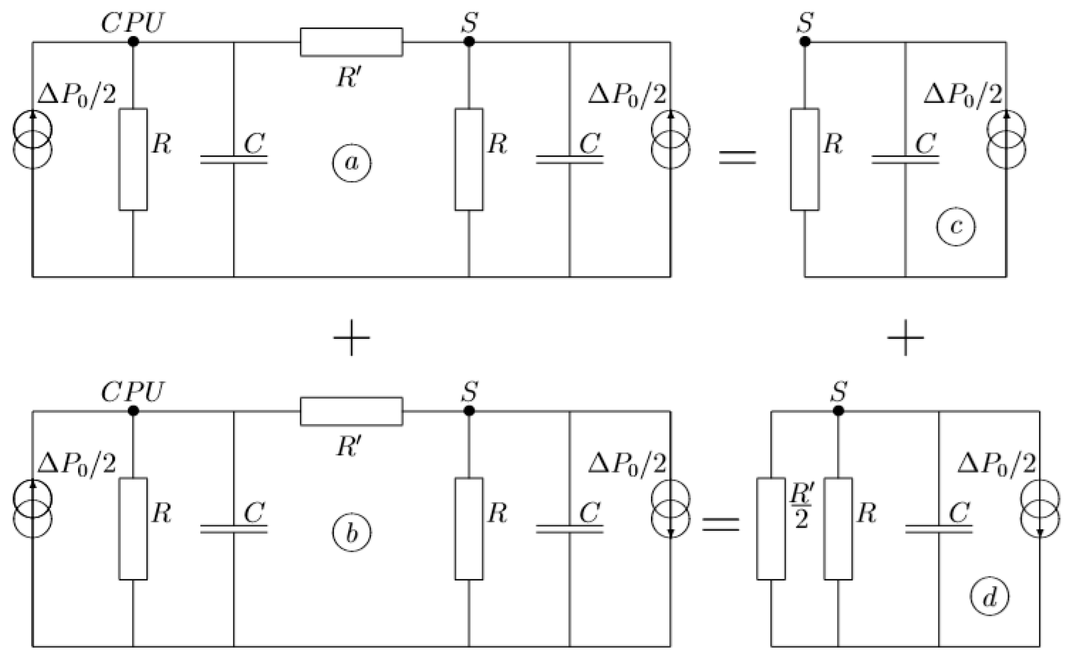
The easiest way to solve the network of Figure 3 is to use the so-called symmetrical components. One will notice that, apart from the current source, the network shown in Figure 3 is symmetrical.
Hence, the network can be represented as the superposition of two networks (a and b) shown in Figure A1. On the right-hand side, opposite current sources were introduced so that the total current remained zero. The network of Figure A1a is perfectly symmetrical so that no current can flow through the resistor R’. Hence, the network of Figure A1a is equivalent to the network of Figure A1c. The network of Figure A1b is antisymmetrical, which means that the middle of the resistor R’ is always at zero potential. Consequently, this network is equivalent to the network shown in Figure A1d. At last, we just have to solve the networks of Figure A1c,d. Both are simple RC networks that can be easily solved by inspection. Immediately, one finds the time constants of Equation (3). Adding the two solutions gives rise to the relation in Equation (2).
Figure A1.
Equivalent thermal network represented as the superposition of a symmetrical and an antisymmetrical network.
Figure A1.
Equivalent thermal network represented as the superposition of a symmetrical and an antisymmetrical network.
References
- Long, J.; Ogrenci-Memik, S.; Memik, G.; Mukherjee, R. Thermal monitoring mechanisms for chip multiprocessors. ACM Trans. Arch. Code Optim. 2008, 5, 1–33. [Google Scholar] [CrossRef] [Green Version]
- Memik, S.O.; Mukherjee, R.; Ni, M.; Long, J. Optimizing Thermal Sensor Allocation for Microprocessors. IEEE Trans. Comput. Des. Integr. Circuits Syst. 2008, 27, 516–527. [Google Scholar] [CrossRef]
- Huang, W.; Stan, M.R.; Skadron, K.; Sankaranarayanan, K.; Ghosh, S.; Velusam, S. Compact thermal modeling for temperature-Aware design. In Proceedings of the the 41st annual Design Automation Conference, San Diego, CA, USA, 19–23 July 2004; pp. 878–883. [Google Scholar]
- Samake, A.; Kocanda, P.; Kos, A. Effective approach of microprocessor throughput enhancement. Microelectron. Int. 2019, 36, 14–21. [Google Scholar] [CrossRef]
- Samake, A.; Kocanda, P.; Kos, A. Improvement of microsystem throughput using new cooling system. Sci. Lett. Rzeszow Univ. Technol. Electrotech. 2016, XXIV, 5–15. [Google Scholar] [CrossRef] [Green Version]
- Poppe, A.; Szekely, V. Dynamic temperature measurements: Tools providing a look into package and mount structures. Electron. Cool. 2002, 8, 10–18. [Google Scholar]
- Székely, V.; Van Bien, T. Fine structure of heat flow path in semiconductor devices: A measurement and identification method. Solid-State Electron. 1988, 31, 1363–1368. [Google Scholar] [CrossRef]
- Szekely, V. On Representation of infinite-Length distributed RC one-Ports. IEEE Trans. Circuits Syst. 1991, 38, 711–719. [Google Scholar] [CrossRef]
- Simon, D.; Boianceanu, C.; De Mey, G.; Topa, V. Experimental Reliability Improvement of Power Devices Operated under Fast Thermal Cycling. IEEE Electron Device Lett. 2015, 36. [Google Scholar] [CrossRef] [Green Version]
- Simon, D.; Boianceanu, C.; De Mey, G.; Topa, V.; Spitzer, A. Reliability Analysis for Power Devices Which Undergo Fast Thermal Cycling. IEEE Trans. Device Mater. Reliab. 2016, 16, 336–344. [Google Scholar] [CrossRef]
- Janicki, M.; de Mey, G.; Napieralski, A. Transient thermal analysis of multilayered structures using Green’s functions. Microelectron. Reliab. 2002, 42, 1064–1069. [Google Scholar] [CrossRef]
- Janicki, M.; De Mey, G.; Napieralski, A. Application of Green’s functions for analysis of transient thermal states in electronic circuits. Microelectron. J. 2002, 33, 733–738. [Google Scholar] [CrossRef]
- Janicki, M.; Banaszczyk, J.; De Mey, G.; Kamiński, M.; Vermeersch, B.; Napieralski, A. Dynamic thermal modelling of a power integrated circuit with the application of structure functions. Microelectron. J. 2009, 40, 1135–1140. [Google Scholar] [CrossRef]
- Janicki, M.; Banaszczyk, J.; Vermeersch, B.; De Mey, G.; Napieralski, A. Generation of reduced dynamic thermal models of electronic systems from time constant spectra of transient temperature responses. Microelectron. Reliab. 2011, 51, 1351–1355. [Google Scholar] [CrossRef]
- Kawka, P.; de Mey, G.; Vermeersch, B. Thermal characterisation of electronics packages using the Nyquist plot of the thermal impedance. IEEE Trans. Compon. Packag. Technol. 2007, 30, 660–665. [Google Scholar] [CrossRef]
- De Mey, G.; Pilarski, J.; Wojcik, M.; Lasota, M.; Banaszczyk, J.; Vermeersch, B.; Napieralski, A. Influence of interface materials on the thermal impedance of electronic packages. Int. Commun. Heat Mass Transf. 2009, 36, 210–212. [Google Scholar] [CrossRef]
- Vermeersch, B.; De Mey, G. Thermal impedance plots of micro-scaled devices. Microelectron. Reliab. 2006, 46, 174–177. [Google Scholar] [CrossRef] [Green Version]
- Vermeersch, B.; De Mey, G. Influence of substrate thickness on thermal impedance of microelectronic structures. Microelectron. Reliab. 2007, 47, 437–443. [Google Scholar] [CrossRef] [Green Version]
- De Mey, G.; Vermeersch, B.; Banaszczyk, J.; Swiatczak, T.; Wiecek, B.; Janicki, M.; Napieralski, A. Thermal impedances of thin plates. Int. J. Heat Mass Transf. 2007, 50, 4457–4460. [Google Scholar] [CrossRef]
- Vermeersch, B.; De Mey, G. A Fixed-Angle Dynamic Heat Spreading Model for (An)Isotropic Rear-Cooled Substrates. J. Heat Transf. 2008, 130, 121301. [Google Scholar] [CrossRef]
- Chatziathanasiou, V.; Chatzipanagiotou, P.; Papagiannopoulos, I.; de Mey, G.; Wiecek, B. Dynamic thermal analysis of underground medium power cables using thermal impedance, time constant distribution and structure function. Appl. Therm. Eng. 2013, 60, 256–260. [Google Scholar] [CrossRef]
- Więcek, B.; De Mey, G.; Chatziathanasiou, V.; Papagiannakis, A.; Theodosoglou, I. Harmonic analysis of dynamic thermal problems in high voltage overhead transmission lines and buried cables. Int. J. Electr. Power Energy Syst. 2014, 58, 199–205. [Google Scholar] [CrossRef]
- Chatzipanagiotou, P.; Chatziathanasiou, V.; De Mey, G.; Więcek, B. Influence of soil humidity on the thermal impedance, time constant and structure function of underground cables: A laboratory experiment. Appl. Therm. Eng. 2017, 113, 1444–1451. [Google Scholar] [CrossRef]
- Papagiannopoulos, I.; Chatziathanasiou, V.; Exizidis, L.; Andreou, G.; de Mey, G.; Wiecek, B. Behaviour of the thermal impedance of buried power cables. Int. J. Electr. Power Energy Syst. 2013, 44, 383–387. [Google Scholar] [CrossRef]
- Kałuża, M.; Więcek, B.; De Mey, G.; Hatzopoulos, A.; Chatziathanasiou, V. Thermal impedance measurement of integrated inductors on bulk silicon substrate. Microelectron. Reliab. 2017, 73, 54–59. [Google Scholar] [CrossRef]
- Legierski, J.; Więcek, B.; De Mey, G. Measurements and simulations of transient characteristics of heat pipes. Microelectron. Reliab. 2006, 46, 109–115. [Google Scholar] [CrossRef]
- De Mey, G.; Wyrzutowicz, J.; De Vos, A.; Marańda, W.; Napieralski, A. Influence of lateral heat diffusion on the thermal impedance measurement of photovoltaic panels. Sol. Energy Mater. Sol. Cells 2013, 112, 1–5. [Google Scholar] [CrossRef] [Green Version]
Figure 1.
Microprocessor activity and CPU/GPU temperature.

Figure 2.
Experimental recorded CPU temperature Texp (●) compared with an analytical function Tfitt.
Figure 2.
Experimental recorded CPU temperature Texp (●) compared with an analytical function Tfitt.
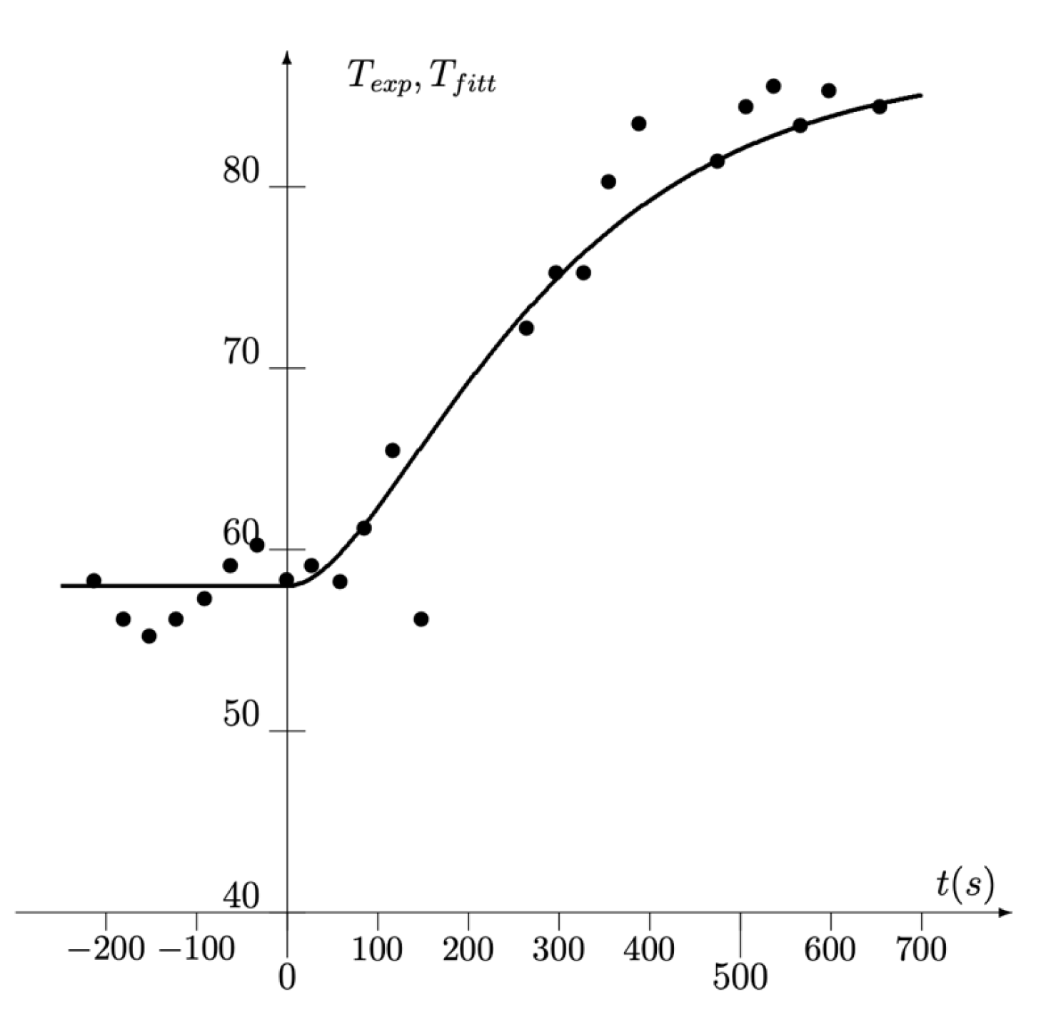
Figure 3.
Equivalent thermal network. ΔTCPU and ΔTS are temperature rises above the reference (=58°).
Figure 3.
Equivalent thermal network. ΔTCPU and ΔTS are temperature rises above the reference (=58°).
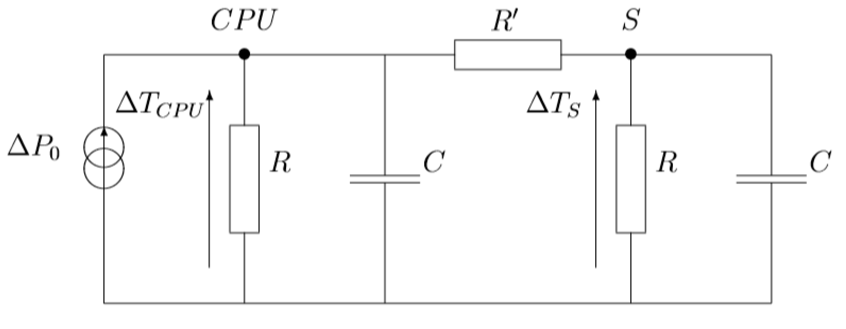
Figure 4.
CPU and sensor temperature versus time.

© 2020 by the authors. Licensee MDPI, Basel, Switzerland. This article is an open access article distributed under the terms and conditions of the Creative Commons Attribution (CC BY) license (http://creativecommons.org/licenses/by/4.0/).
Share and Cite
MDPI and ACS Style
De Mey, G.; Kos, A. The Influence of an Additional Sensor on the Microprocessor Temperature. Energies 2020, 13, 3156. https://doi.org/10.3390/en13123156
AMA Style
De Mey G, Kos A. The Influence of an Additional Sensor on the Microprocessor Temperature. Energies. 2020; 13(12):3156. https://doi.org/10.3390/en13123156
Chicago/Turabian StyleDe Mey, Gilbert, and Andrzej Kos. 2020. "The Influence of an Additional Sensor on the Microprocessor Temperature" Energies 13, no. 12: 3156. https://doi.org/10.3390/en13123156
Note that from the first issue of 2016, this journal uses article numbers instead of page numbers. See further details here.