Fast Heuristic AC Power Flow Analysis with Data-Driven Enhanced Linearized Model

Abstract

Though the full AC power flow model can accurately represent the physical power system, the use of this model is limited in practice due to the computational complexity associated with its non-linear and non-convexity characteristics. For instance, the AC power flow model is not incorporated in the unit commitment model for practical power systems. Instead, an alternative linearized DC power flow model is widely used in today’s power system operational and planning tools. However, DC power flow model will be useless when reactive power and voltage magnitude are of concern. Therefore, a linearized AC (LAC) power flow model is needed to address this issue. This paper first introduces a traditional LAC model and then proposes an enhanced data-driven linearized AC (DLAC) model using the regression analysis technique. Numerical simulations conducted on the Tennessee Valley Authority (TVA) system demonstrate the performance and effectiveness of the proposed DLAC model.

1. Introduction

The power system is one of the most complicated physical networks in the world. Almost all electricity demands are served through power systems. It is of utmost importance to study the fundamentals of power systems including power flow analysis. Power flow model is involved in a great number of problems and is incorporated in various application models. For instance, it is incorporated into the formulations of state estimation [1,2], security-constrained economic dispatch [3,4,5], security-constrained unit commitment [6,7], transmission maintenance scheduling [8], and transmission expansion planning [9,10,11,12]. Hence, power flow analysis is remarkably important for power system planning as well as power system operations. Currently, the two most popular power flow models are the full AC model and the linearized DC model.

The full AC power flow model, following Kirchhoff’s circuit laws and Ohm’s law, can accurately represent the physical power system. This model captures all electric variables of interest, including active power, reactive power, phase angle and voltage magnitude. However, it is not uncommon to observe the divergence of AC power flow problems even with commercial software such as PSS/E and DSATools. In addition, incorporating AC power flow model into an optimization model will make it impossible to solve.

Though a number of algorithms were proposed in literature to improve the convergence performance of the AC power flow model [13,14], it still remains to be an unresolved issue. The computational complexity due to its non-linearity and non-convexity makes it impossible to use the AC power flow model in a variety of optimization problems. For instance, though the classical formulation for AC model based economic dispatch was first created by Carpentier in 1962 [15], no robust and reliable algorithm has been developed since then to solve the problem in a timely manner due to its non-linearity, non-convexity, and large-scale features. As a result, the industry today still uses a linearized DC power flow model that ignores reactive power and voltage magnitude.

To relieve computational burden, the simplified traditional DC power flow model is adopted when only active power and phase angle are of concern. As the DC model is simple, efficient, and reliable, it is widely used in the power industry and many power system applications [16,17,18,19,20]. For instance, instead of the AC model, the DC model is employed in the day-ahead energy markets and real-time energy markets.

The DC model is a good approximation of the AC model in terms of active power solution for high voltage transmission networks, of which the X/R ratios are typically very high. However, DC power flow may fail to perform properly in some scenarios. For instance, the work in [21] shows that DC model based cascading failure simulators fail to capture the power system behaviors in several circumstances. Though the average error for active power is limited to 5%, significant errors are still observed on several individual lines [22]. Three DC power flow models are investigated in [23]. It is concluded that the α-matching model has the most accurate results. However, α-matching method is hot-start, and thus its utilization is only restricted to near-real-time applications with the knowledge of initial system status. Furthermore, DC model cannot be utilized in the cases that voltage magnitude and reactive power are of interest.

Though the full AC power flow model is accurate, its computational complexity and unstable characteristics restrict its utilization. DC power flow model can reduce the computational burden significantly, but it may suffer from an inaccuracy issue and report no information regarding reactive power and voltage magnitude. Therefore, for situations when the reactive power and voltage information are needed while the solution time is limited, a fast linearized AC (LAC) power flow model that can capture reactive power and voltage magnitude is desired.

Three linear-programming AC power flow models, derived with polyhedral relaxation and Taylor series, are proposed in [24]. Numerical simulation demonstrates the effectiveness of the proposed models. Another linear approximation of the AC model is presented in [25]. The error of this approximation is less than 6% for voltage magnitude. It is worth noting that the approximation error of the proposed model in this paper is only about 1%. A linear relaxation of AC power flow model using polynomial optimization is proposed in [26]. The linearized model is applied to transmission planning problem, and the case studies demonstrate its capability of obtaining approximate solutions in a reasonable time. However, the solution is not checked and compared with the accurate full AC model. An iterative linear power flow method proposed in [27] seems to be accurate and fast. However, this iterative method may fail to converge. All the above work [24,25,26,27] is demonstrated on small-scale standard test cases only, and further efforts are needed to investigate the model accuracy on large-scale practical power systems.

To solve the scalability and accuracy issues related to AC power flow linearization, a data-driven linearized AC (DLAC) power flow model is proposed in this paper. This model captures all system state variables including active power, phase angle, reactive power and voltage magnitude. First, a regular linearization of full AC power flow model is conducted by ignoring higher order terms. Then, coefficients are assigned to the terms that remain in the model. The regression analysis technique is performed to determine those coefficients, which can reflect the system’s typical or recent status. The philosophy behind this idea is that the system condition does not change significantly in a short timeframe such as a day. For instance, generator voltage setting points typically do not change or change within very narrow ranges, which indicates that voltage magnitude for other neighboring buses would also not change significantly. Another noticeable fact is that the voltage magnitudes for high voltage transmission networks are typically higher than one per unit.

The proposed enhanced DLAC power flow model can (i) substantially reduce the error associated with active power flows as compared with the traditional DC power flow model; (ii) and obtain much more accurate voltage profile and significantly improve reactive power flow solutions as compared with the traditional linearized AC model. In addition, the proposed DLAC model can be easily incorporated in various power system applications such as day-ahead unit commitment or real-time economic dispatch, which can substantially improve their performance. The effectiveness of the proposed DLAC model is demonstrated with a practical U.S. power system.

The rest of this paper is organized as follows. Section 2 presents an overview on the power flow model. Section 3 introduces the regression analysis technique. Section 4 discusses the regular LAC model and the proposed enhanced DLAC model. Case studies are presented in Section 5. Finally, Section 6 concludes the paper.

2. AC Power Flow Model

Power flow studies are the basis of power system analysis [28]. The per unit system and single-line diagram are usually used for simplification. In the power flow studies, the following assumptions are typically made:

• The system is three-phase balanced and thus, only the positive sequence network is of concern.
• The Pi-equivalent circuit model can accurately represent the transmission network.
• Individual generation and load are known except for the generation at the slack bus.

Given these assumptions, the following state variables can be obtained by solving an AC power flow problem through computer programs:

• voltage magnitude and phase angle at each bus,
• active power and reactive power generations at each bus,
• active power flow and reactive power flow in both directions on each branch,
• loss on each branch.

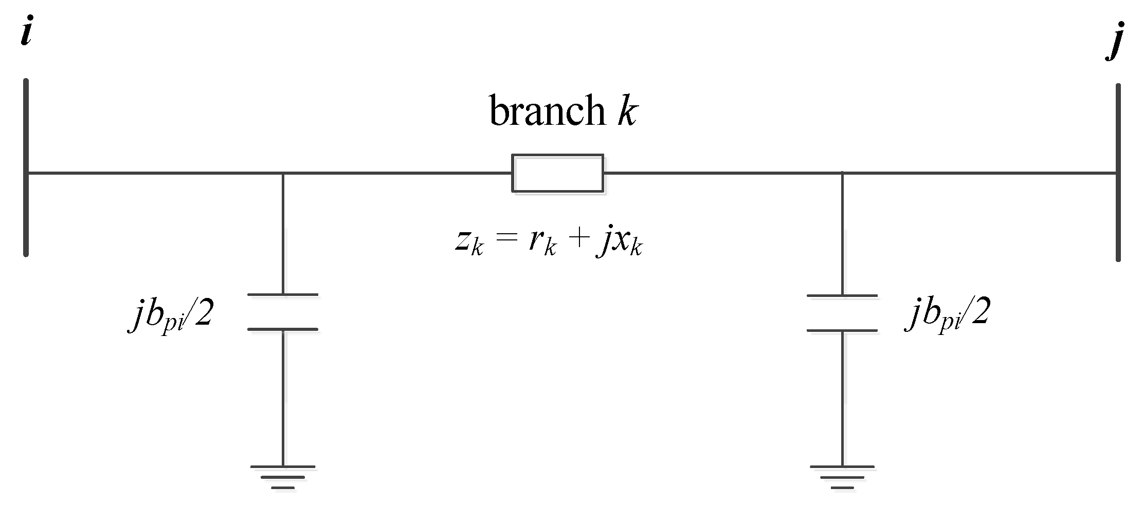
Figure 1 shows the single-line diagram of a two-terminal circuit. A power system network consists of a number of those 2-terminal circuits. Note that $P$ denotes active power while $Q$ stands for reactive power. Normally, the power flowing out of one end-bus does not equal to the power flowing into the other bus because of (i) the reactive power produced by transmission lines, and (ii) the losses on the branch connected to the two end buses, which means that $P_{ij}\ne -P_{ji}$ and $Q_{ij}\ne -Q_{ji}$.

The power flow equations for a branch are given below.

$$P_{ij}=V_i^2{g}_{ij}-V_i{V}_j\left(g_{ij}cos{\theta }_{ij}+b_{ij}sin{\theta }_{ij}\right)$$

(1)

$$Q_{ij}=-V_i^2\left(b_{ij}+\frac{b_{pi}}{2}\right)+V_i{V}_j\left(b_{ij}cos{\theta }_{ij}-g_{ij}sin{\theta }_{ij}\right)$$

(2)

where $P_{ij}$ and $Q_{ij}$ denote the active power and reactive power on branch k flowing from bus i to bus j respectively, ${\theta }_{ij}$ denotes the phase angle difference across this branch, while $V_i$ and $V_j$ are the voltage magnitude of bus i and bus j, respectively. $y_{ij}$ and $b_{pi}$ denote the series admittance and parallel susceptance of Pi-equivalent circuit respectively. $g_{ij}$ and $b_{ij}$ are the real part and imaginary part of $y_{ij}$ respectively, and they can be calculated with the following equation,

$$y_{ij}=g_{ij}+j{b}_{ij}=\frac{1}{z_{ij}}=\frac{1}{r_{ij}+j{x}_{ij}}=\frac{r_{ij}-j{x}_{ij}}{r_{ij}^2+x_{ij}^2}$$

(3)

where $z_{ij}$, $r_{ij}$, and $x_{ij}$ denote line impedance, resistance and reactance of the Pi-equivalent circuit respectively.

Other important equations for the power flow studies are the nodal power balance constraints as shown in Equations (4) and (5).

$$P_{ig}-P_{id}-{\displaystyle \sum }_{h\in S_{i+}}{P}_{ih}+{\displaystyle \sum }_{h\in S_{i-}}{P}_{hi}=0$$

(4)

$$Q_{ig}-Q_{id}-{\displaystyle \sum }_{h\in S_{i+}}{Q}_{ih}+{\displaystyle \sum }_{h\in S_{i-}}{Q}_{hi}=0$$

(5)

where $S_{i+}$ denotes the set of buses that are directly connected to bus i when bus i is designated as the sending end, and $S_{i-}$ denotes the set of buses that are directly connected to bus i when bus i is designated as the receiving end. $P_{ig}$ and $Q_{ig}$ represent the total active power and total reactive power produced by the generators at bus i, respectively, $P_{id}$ and $Q_{id}$ are the total active power load and total reactive power load at bus i respectively. $P_{ih}$ and $Q_{ih}$ denote the branch active power and reactive power flowing from bus i to bus h respectively.

3. Regression Analysis

Regression analysis is a widely used statistical technique for estimating the relationships among variables and determining the model for those variables [29,30]. It typically involves a dependent variable that is also referred to as a response variable, and one or multiple independent variables that are often called as regressors or predictors. The most popular method is the least squares approximation. A general multiple linear regression model with k regressors is defined as follows:

$$y={\beta }_0+{\displaystyle \sum }_{j=1}^k{\beta }_j{x}_j+\epsilon$$

(6)

where $x_j$ is the j^th regressor, $\beta$ denotes the coefficient, and $\epsilon$ denotes the error.

Provided a sample set of n observations, all parameters ${\beta }_j$ can be determined as ${\widehat{\beta }}_j$ through regression analysis. The estimated value ${\widehat{y}}_i$ and residual $e_i$ for the i^th observation in the sample space are defined as Equations (7) and (8) respectively.

$${\widehat{y}}_i={\widehat{\beta }}_0+{\displaystyle \sum }_{j=1}^k{\widehat{\beta }}_j{x}_{ij}$$

(7)

$$e_i=y_i-{\widehat{y}}_i$$

(8)

where $y_i$ is the observed value of the i^th observation. Residual $e$ denotes the difference between the observed value and the estimated or fitted value while error $\epsilon$ represents the discrepancy between the observed value and the true value.

After creating a regression model, it is important to (i) conduct model adequacy checking to ensure the model fits the data and (ii) perform model validation to demonstrate the effectiveness of the regression model.

3.1. Model Adequacy Checking

One statistical metric to evaluate the overall model adequacy is the Coefficient of Determination, which is a percentage number denoted as $R^2$. $R^2$ quantifies how good the regression model is and how much variation can be explained with the regression model. In other words, $R^2$ is the proportion of variation in the response variable explained and predicted by the regressors. 100% indicates that the regression model explains all the variability around the mean. $R^2$ is defined in the equation below,

$$R^2=1-\frac{S{S}_{res}}{S{S}_{total}}$$

(9)

where $S{S}_{res}$ denotes the residual sum of squares and $S{S}_{total}$ denotes the total sum of squares.

Residual analysis can effectively discover several types of model inadequacies and measure how good the regression model fits the data [30]. Scaled residuals such as standardized residuals may be a better analysis technique to find outliers and analyze the regression model. The standardized residuals with zero mean and approximately unit variance is defined in the equation below,

$$d_i=e_i/\sqrt{M{S}_{Res}}$$

(10)

where $M{S}_{Res}$ is the residual mean square that estimates the average variance of residuals.

Another commonly used scaled residual is the R-student residual, defined in Equation (11) shown below. R-student residuals are often used since their variance is constant.

$$t_i=e_i/\sqrt{S_{\left(i\right)}^2\left(1-h_{ii}\right)}$$

(11)

where $h_{ii}$ is an element of the hat matrix and $S_{\left(i\right)}^2$ denotes the estimate of variance with the i^th observation being moved from the dataset.

A plot of the residuals against the fitted values can help detect several types of model inadequacy. If the residuals in the plot are contained in a horizontal band, then, there is no indication of model deficiency. If the residuals against fitted values form a pattern such as a funnel, double bow, or nonlinear, then it indicates that defects may exist in the regression model and further investigation is required.

3.2. Model Validation

In the regression analysis domain, the best fitted model to the sample dataset may not accurately describe the relationship between variables. One key concern is the danger of extrapolation. Though a regression model is often used for extrapolation, it does not apply to the power flow analysis since the power system status does not change significantly especially in a short time frame. The case studies section in this paper demonstrate that the proposed regression model for linearized power flow equations has very similar performance in different system scenarios.

Multicollinearity may occur when regressors are highly linearly dependent and it has serious negative effects on the regression model. The regression coefficients may be poorly estimated when multicollinearity exists, which may result in inaccuracy of the regression model. One popular technique to detect multicollinearity is variance inflation factor (VIF). VIF measures how much variance of the estimated regressor coefficient is inflated. Each regressor in the regression model corresponds to one VIF value. This will be very useful to determine whether that regressor is involved in multicollinearity. High VIF indicates the associated regressor may have poor coefficient. VIFs below 3 suggests multicollinearity does not exist [31]. A VIF of one means there is no correlation between the associated regressor and the other regressors.

4. Data-Driven Linearized Power Flow Model

The regression analysis technique is often used for determining the causal effect relationship between the variables. With a power engineering insight, this work uses regression analysis technique to improve the simplified model derived from linearization of the complex full AC power flow model. This section first presents the traditional DC model and regular linearized AC model. Then, it describes the proposed data-driven DC (DDC) model and the proposed data-driven linearized AC model that can capture recent or historical system status with regression analysis.

4.1. DC Power Flow Model

The most commonly used linearized power flow model is the DC power flow model represented by the equation shown below. This DC power flow model can be used for applications when voltage magnitude and reactive power are not of concern. Due to its linearity and low computational burden, the DC power flow model is widely used in academic studies, as well as industry practices.

$$P_{ij}={\theta }_{ij}/x_{ij}$$

(12)

4.2. Linearized AC Power Flow Model

Though DC power flow model has been widely used for dozens of years, it does not apply for the scenarios when voltage and reactive power are of concern. Therefore, a linearized AC power flow model can be very useful. The nodal voltage magnitude can be written as follows [32],

$$V_i=1+\Delta V_i$$

(13)

where $\Delta V_i$ is supposed to be very small since nodal voltage is very close to one in normal situations. Substituting Equation (13) into Equations (1) and (2) and ignoring the second order terms including $\Delta V_i{\theta }_{ij}$ and $\Delta V_j{\theta }_{ij}$, we can obtain:

$$P_{ij}=-{\theta }_{ij}{b}_{ij}+\left(\Delta V_i-\Delta V_j\right)g_{ij}$$

(14)

$$Q_{ij}=-\left(1+2\Delta V_i\right)b_{pi}-{\theta }_{ij}{g}_{ij}-\left(\Delta V_i-\Delta V_j\right)b_{ij}$$

(15)

Then, substituting $\Delta V_i=V_i-1$, derived from Equation (13), back into Equations (14) and (15), we will obtain the linearized AC power flow equations shown below.

$$P_{ij}=-{\theta }_{ij}{b}_{ij}+\left(V_i-V_j\right)g_{ij}$$

(16)

$$Q_{ij}=b_{pi}-2V_i{b}_{pi}-{\theta }_{ij}{g}_{ij}-\left(V_i-V_j\right)b_{ij}$$

(17)

4.3. Data-Driven Linearized DC and AC Power Flow Models

In the simplification of the DC power flow model represented by Equation (12), voltage magnitude is assumed to be one per unit all over the entire system, which is one of the main sources why DC power flow model is not very accurate. It would be very useful if a more accurate model with similar computational complexity is available. Thus, this paper presents a data-driven DC power flow model that uses the regression analysis technique to capture the system specific condition and reflect it with different coefficients in the model. Thus, as shown in Equation (18), instead of having the proportional coefficient being one, we can adjust it and optimize it based on the system recent and historical status.

$$P_{ij}=K_D{\theta }_{ij}/x_{ij}$$

(18)

Similarly, adjustments to the LAC model can be made to improve the model by incorporating the system recent and/or historical status. The data-driven LAC model with coefficients associating to each term is shown below. Model Equation (19) represents regression model P while Equation (20) denotes regression model Q. The constant term in Equation (20) is the intercept of the regression model Q. As compared to the regular LAC model described in Section 4.2, the proposed DLAC model has better performance and smaller model error.

$$P_{ij}=-K_{A1}{\theta }_{ij}{b}_{ij}+K_{A2}\left(V_i-V_j\right)g_{ij}$$

(19)

$$Q_{ij}=b_{pi}-2K_{A3}{V}_i{b}_{pi}-K_{A4}{\theta }_{ij}{g}_{ij}-K_{A5}\left(V_i-V_j\right)b_{ij}$$

(20)

The proposed DDC and DLAC models have several advantages over other regression models. Unlike [33,34], the numbers of regressors in the proposed regression models Equations (18)–(20) do not increase with the size of the system, which enables the proposed DDC and DLAC models to be computationally efficient. As compared with the regular LAC model Equations (16)–(17), the proposed DLAC model Equations (19)–(20) shares very similar computational complexity since they have the same number of linear algebra equations. The addition of coefficients does not create substantial computational complexity. In addition, the proposed regression models are derived from the physical model and the regressors are not correlated. For instance, for the proposed regression model Q, each data entry includes the voltage magnitude of only one end bus of a line rather than two end buses of a line, which avoids potential correlation across regressors. To summarize, the proposed DDC and DLAC models have neither scalability nor collinearity issues.

4.4. Metrics

The approximation error of the simplified power flow heuristic model is defined in Equation (21) below,

$${ϵ}_m=\frac{1}{N_m}{\displaystyle \sum }_{i=1}^{N_m}\left|\frac{x_m^i-x_{AC}^i}{x_{AC}^i}\right|\ast 100\%$$

(21)

where $x_m$ denotes the state variable for a simplified power flow model m while $x_{AC}$ denotes the same state variable obtained with the full AC model. $i$ indicates the i^th element while $N_m$ denotes the number of elements in $x_m$ or $x_{AC}$.

To quantify how much the proposed data-driven model improves the solution accuracy against the traditional model, a model improvement index, a percentage number, is defined in Equation (22).

$${\eta }_{b,a}=\frac{{ϵ}_a-{ϵ}_b}{{ϵ}_a}\ast 100\%$$

(22)

In addition to analyzing the model improvement index, the sum and the average of absolute deviations across all buses of interest or all branches of interest are important indicators on the performance of heuristic models. The sum of absolute deviation for model m is defined in Equation (23) while the average of absolute deviations is defined in Equation (24).

$$s_m={\displaystyle \sum }_{i=1}^{N_m}\left|x_m^i-x_{AC}^i\right|$$

(23)

$${\gamma }_m=\frac{1}{N_m}{\displaystyle \sum }_{i=1}^{N_m}\left|x_m^i-x_{AC}^i\right|$$

(24)

5. Case Studies

The proposed data-driven DC model and data-driven linearized AC model are tested against the practical Tennessee Valley Authority (TVA) system and compared with the traditional full AC power flow model and simplified DC power flow model. TVA is a U.S. federally owned corporation that covers a population of about 10 million people [35].

This system has 1779 buses and 2301 branches. There are 72 consecutive hourly cases that covers 3 days’ scenarios [36]; they are used as the test cases in this work. They are referred to as hour 1 case, hour 2 case, …, and hour 72 case in this paper. AC power flow simulation is conducted on hour 1 case to obtain the system status that is used as the training data for regression analysis: the data used for determining the coefficient for data-driven DC model are line reactance, line active power flow and phase angle difference across the line; the data used for determining the coefficients for data-driven linearized AC model include line reactance and susceptance, line active power flow and reactive power flow, phase angle difference across the line, and voltage magnitudes at two end buses. The other cases are used to validate the proposed models. In this work, R is used as the statistical tool to perform regression analysis [37].

5.1. Data-Driven DC Model

With the power flow results obtained from the full AC power flow simulation on hour 1 case, regression analysis determines the coefficient $K_D$ in Equation (18) to be 1.12, which is above one unit. This is consistent with the fact that the average voltage magnitude for the same hour 1 case is 1.04 which is also above one unit.

The coefficient of determination for this regression model is 0.9964. This indicates that the regression model, $P_{ij}=1.12{\theta }_{ij}/x_{ij}$, can explain 99.64% of the variation of the response variable $P_{ij}$. VIF does not apply to regression model with one single regressor. Thus, the DDC model won’t have any multicollinearity or overfitting issues as it has only one single regressor.

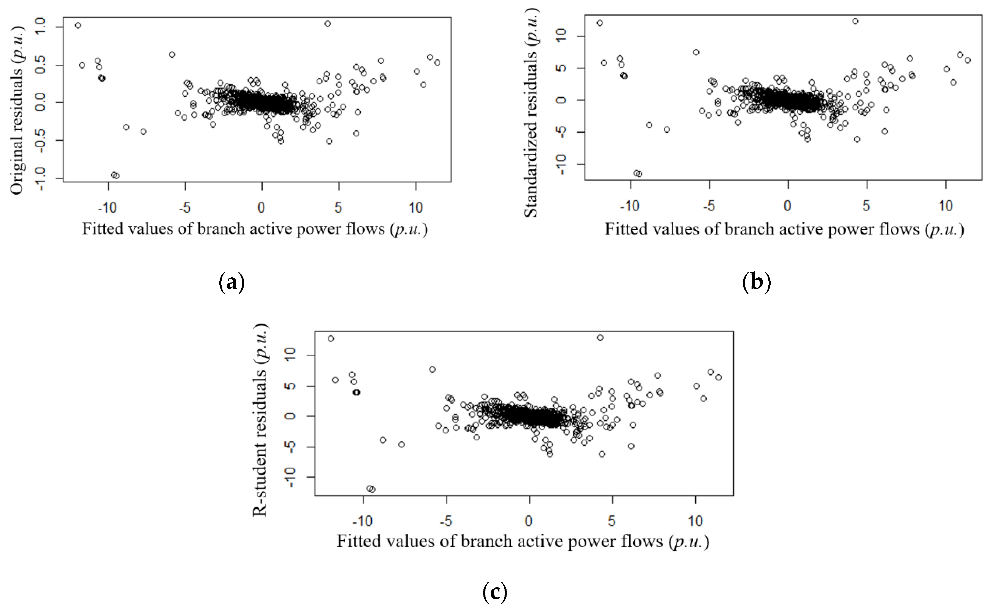
Figure 2 shows the plots of different types of residuals against the fitted values of branch active power flows for the hour 1 case. The residuals in Figure 2a–c correspond to the original residuals, standardized residuals, and R-student residuals, respectively. Note that the residual scale for Figure 2b,c is about 10 times larger than Figure 2a since Figure 2b,c show scaled residuals while Figure 2a does not. In Figure 2a, majority of the original residuals reside within the range of [−0.2, 0.2] and very few of them goes beyond the boundary of [−0.5, 0.5]. This indicates the errors of the regression model are within an acceptance range. Similarly, Figure 2b,c show that the residuals are mostly located within 3 units of the standard deviation. In conclusion, Figure 2 illustrates the effectiveness of the DDC power flow model.

Note that $K_D{\theta }_{ij}$ in Equation (18) is mathematically equivalent to ${\theta }_{ij}$ in Equation (12); in other words, the proposed DDC model will achieve the same $P_{ij}$ while it can improve the solution for ${\theta }_{ij}$. The power flow solutions obtained from the DC model and the DDC model for the TVA system condition represented by hour 1 case are presented in

Table 1. Results with DDC and DC Models for Hour 1 Case.

		$\mathbf{Tolerance}\mathbf{in}\mathbf{MW}\mathbf{for}{\mathit{P}}_{\mathit{i}\mathit{j}}$
		1	5	10	50
# of branches		2093	1973	1746	841
$P_{ij}$	${ϵ}_{DC}$	8.75%	6.59%	5.45%	3.66%
	${ϵ}_{DDC}$	8.75%	6.59%	5.45%	3.66%
${\theta }_{ij}$	${ϵ}_{DC}$	22.1%	17.4%	13.4%	11.2%
	${ϵ}_{DDC}$	16.9%	12.6%	8.4%	5.2%
	${\eta }_{DDC,DC}$	23.6%	27.8%	37.0%	53.2%

. The branch active power P calculated from both models are the same while the improvement on ${\theta }_{ij}$ is significant. The improvement for branches with flows of over 50 MW is more than 50% on average. As shown in

Table 2. Results with DDC and DC Models for Hour 2 Case.

		$\mathbf{Tolerance}\mathbf{in}\mathbf{MW}\mathbf{for}{\mathit{P}}_{\mathit{i}\mathit{j}}$
		1	5	10	50
# of branches		2082	1954	1722	815
$P_{ij}$	${ϵ}_{DC}$	6.96%	5.00%	4.28%	2.94%
	${ϵ}_{DDC}$	6.96%	5.00%	4.28%	2.94%
${\theta }_{ij}$	${ϵ}_{DC}$	18.0%	15.6%	11.2%	10.0%
	${ϵ}_{DDC}$	13.8%	11.6%	7.18%	5.20%
	${\eta }_{DDC,DC}$	22.9%	26.0%	36.0%	48.2%

, very similar results are observed for hour 2 case, which represents a different scenario with the one used to train the DDC model. This further demonstrates that the proposed DDC model can substantially improve ${\theta }_{ij}$ as compared to the traditional DC model.

5.2. Data-Driven Linearized AC Model

In the DLAC model, two separate regression models are built for branch active power and reactive power respectively. The results of coefficients are presented in

Table 3. Coefficients of the Regression Models.

Coefficient		${\mathit{K}}_{\mathit{A}1}$	${\mathit{K}}_{\mathit{A}2}$	${\mathit{K}}_{\mathit{A}3}$	${\mathit{K}}_{\mathit{A}4}$	${\mathit{K}}_{\mathit{A}5}$
Estimate		1.12	0.98	0.87	1.02	1.01
95% CI	2.5%	1.12	0.93	0.85	1.01	1.00
	97.5%	1.12	1.03	0.88	1.02	1.04

Note that CI denotes confidence interval.

. All five coefficients deviate from the value of one that is used for the regular LAC model. The 95% confidence interval for each regression coefficient is very narrow, which indicates that the coefficients are very stable and accurate for the given dataset or system conditions.

As presented in

Table 4. Results of Regression Analysis.

Regression Model	${\mathit{R}}^2$	VIF
		${\mathit{\theta }}_{\mathit{i}\mathit{j}}{\mathit{b}}_{\mathit{i}\mathit{j}}$	$\left({\mathit{V}}_{\mathit{i}}-{\mathit{V}}_{\mathit{j}}\right){\mathit{g}}_{\mathit{i}\mathit{j}}$	${\mathit{V}}_{\mathit{i}}{\mathit{b}}_{\mathit{p}\mathit{i}}$	${\mathit{\theta }}_{\mathit{i}\mathit{j}}{\mathit{g}}_{\mathit{i}\mathit{j}}$	$\left({\mathit{V}}_{\mathit{i}}-{\mathit{V}}_{\mathit{j}}\right){\mathit{b}}_{\mathit{i}\mathit{j}}$
P	99.74%	1.05	1.05	N/A	NA	NA
Q	98.71%	NA	NA	1.06	1.20	1.16

, the coefficients of determination $R^2$ are 99.74% and 98.71% for the two regression models respectively. This shows that both regression models can explain almost all variance of the branch flows to their means. Table 4 shows the VIFs for the regressors of both regression models are all very small, well below 3, which means that multicollinearity has little effect on the regression models and there is no overfit issue.

Table 5. Statistical results of Multiple Types of Residuals.

Regression Model	e		d		t
	Mean	Variance	Mean	Variance	Mean	Variance
P	0.0020	0.0052	0.027	1.00	0.028	1.05
Q	0.0095	0.0024	0.19	0.96	0.19	1.01

shows that the residual mean of the regression model Q is about five times higher than that of the regression model P. This indicates the proposed DLAC model is more accurate for branch active power than branch reactive power.

Table 6. Analysis of Variance for Response Variable P.

	Df	Sum Sq	Mean Sq	F Value	Pr (>F)
${\theta }_{ij}{b}_{ij}$	1	281.5	281.5	54167	<2.2e-16
$\left(V_i-V_j\right)g_{ij}$	1	4227.1	4227.1	813356	<2.2e-16
Residuals	2299	11.9	0.0052	NA	NA

shows the ANOVA analysis for regression model P, which are used for testing the significance of regression. As the last column indicates, the possibility of the two regressors being insignificance to the response is negligible. In other words, both the terms $\left(V_i-V_j\right)g_{ij}$ and ${\theta }_{ij}{b}_{ij}$ are necessary in regression model P. This implies that DC power flow models with only one term ${\theta }_{ij}{b}_{ij}$ has obvious room for accuracy improvement. This is consistent with the comparison between Table 1 and

Table 7. Results of Active Power with DLAC and LAC for Hour 1 Case.

		$\mathbf{Tolerance}\mathbf{in}\mathbf{MW}\mathbf{for}{\mathit{P}}_{\mathit{i}\mathit{j}}$
		1	5	10	50
# of branches		2093	1973	1746	841
$P_{ij}$	${ϵ}_{LAC}$	6.93%	5.37%	4.43%	3.19%
	${ϵ}_{DLAC}$	7.00%	5.40%	4.46%	3.20%
${\theta }_{ij}$	${ϵ}_{LAC}$	18.3%	14.4%	12.3%	11.3%
	${ϵ}_{DLAC}$	12.2%	8.73%	6.51%	4.71%
	${\eta }_{DLAC,LAC}$	33.6%	39.2%	46.9%	58.5%

. The active power solutions obtained from the LAC and DLAC are very similar, but they are 20% more accurate as compared to the solution obtained with the DC and DDC models. Figure 3 shows the scatter plot for hour 1 case, which indicates the fitted branch active power flows of the proposed DLAC model, are closely in line with the solutions obtained from the full AC model.

Table 7,

Table 8. Results of Reactive Power with DLAC and LAC for Hour 1 Case.

		$\mathbf{Tolerance}\mathbf{in}\mathbf{MVAr}\mathbf{for}{\mathit{Q}}_{\mathit{i}\mathit{j}}$
		1	5	10	50
# of branches		3860	2755	2013	366
$Q_{ij}$	${ϵ}_{LAC}$	64.1%	44.7%	36.0%	32.6%
	${ϵ}_{DLAC}$	42.2%	29.5%	23.6%	22.4%
	${\eta }_{DLAC,LAC}$	34.2%	34.0%	34.5%	31.3%

and

Table 9. Results of Voltage with the DLAC and LAC Models for Hour 1 Case.

		Voltage Level/KV
		All	>=200	(200, 100]	(100, 20]	<20
# of buses		1877	64	1205	192	416
$V_i$	LAC	0.0161	0.0171	0.0188	0.0159	0.0080
	DLAC	0.0105	0.0094	0.0124	0.0106	0.0050
$V_i$%	${ϵ}_{LAC}$	1.54%	1.61%	1.81%	1.54%	0.77%
	${ϵ}_{DLAC}$	1.00%	0.89%	1.19%	1.03%	0.48%
	${\eta }_{DLAC,LAC}$	35.0%	44.7%	34.3%	33.1%	37.7%

, show the statistical results of branch active power, reactive power and bus voltage obtained with DLAC and LAC models on hour 1 case respectively. It is observed that (i) the proposed DLAC model can improve branch reactive power accuracy by 34.5% on branches with flows exceeding 10 MVA and (ii) improve voltage solution by 35.0% against the regular LAC model. As shown in

Table 10. Results of Active Power with DLAC and LAC for Hour 2 Case.

		$\mathbf{Tolerance}\mathbf{for}{\mathit{P}}_{\mathit{i}\mathit{j}}\mathbf{in}\mathbf{MW}$
		1	5	10	50
# of branches		2082	1954	1722	815
$P_{ij}$	${ϵ}_{LAC}$	5.08%	3.98%	3.50%	2.53%
	${ϵ}_{DLAC}$	5.10%	4.01%	3.51%	2.53%
${\theta }_{ij}$	${ϵ}_{LAC}$	16.4%	14.0%	10.8%	10.2%
	${ϵ}_{DLAC}$	10.4%	8.42%	5.55%	4.40%
	${\eta }_{DLAC,LAC}$	36.5%	40.0%	48.7%	57.0%

,

Table 11. Results of Reactive Power with DLAC and LAC for Hour 2 Case.

		$\mathbf{Tolerance}\mathbf{for}{\mathit{Q}}_{\mathit{i}\mathit{j}}\mathbf{in}\mathbf{MVAr}$
		1	5	10	50
# of branches		3811	2747	1996	333
$Q_{ij}$	${ϵ}_{LAC}$	59.4%	42.6%	35.4%	32.0%
	${ϵ}_{DLAC}$	37.9%	27.7%	22.8%	21.1%
	${\eta }_{DLAC,LAC}$	36.2%	35.0%	35.5%	34.1%

and

Table 12. Results of Voltage with DLAC and LAC for Hour 2 Case.

		Voltage Level/KV
		All	>=200	(200, 100]	(100, 20]	<20
# of buses		1877	64	1205	192	416
$V_i$	LAC	0.0153	0.0166	0.0180	0.0152	0.0076
	DLAC	0.0097	0.0089	0.0115	0.0099	0.0045
$V_i$%	${ϵ}_{LAC}$	1.47%	1.56%	1.72%	1.47%	0.73%
	${ϵ}_{DLAC}$	0.93%	0.84%	1.10%	0.96%	0.44%
	${\eta }_{DLAC,LAC}$	36.8%	46.2%	36.1%	34.7%	39.7%

, very similar observations are made from the results by applying both models to hour 2 case. Thus, it is concluded that the proposed DLAC model can significantly improve reactive power accuracy against the regular LAC model, and the active power derived from the LAC/DLAC model is more accurate than the DC/DDC model.

It is important to analyze how much improvement the proposed DLAC model can achieve over the conventional LAC model in terms of branch complex power flow that is used to monitor line loading level against line thermal capacity limit. To avoid the effects of small amount of branch flows, the following analysis focuses on branches that have flows of at least 10 MVA. With this filter, the statistics for hour 1 case and hour 2 case are presented in

Table 13. Statistical Results of Branch Complex Power with Full AC Models with a Tolerance of 10 MVA for Hour 1 Case and Hour 2 Case.

	Min	Max	Mean	Median	s.d.	# of Branches
Hour 1 case	10.0	1189.7	89.9	49.5	135.9	1876
Hour 2 case	10.0	1174.9	86.9	48.0	132.3	1864

. For hour 1 case, the average branch flow error is 5.62% for LAC while it is only 4.65% for DLAC, which corresponds to 17.2% model improvement of DLAC over LAC. For hour 2 case, the average line flow error is 4.77% for LAC while it is 3.85% for DLAC, which corresponds to 19.1% improvement. The sum of absolute deviation in branch complex power flow (SADCP) is also compared for different models. For the traditional LAC model on hour 1 case, the SADCP is 8781 MVA over 1876 branches with an average flow error of 4.68 MVA per branch. With DLAC, the SADCP drops by 16.0% down to 7379 MVA, which correspond to 3.93 MVA per line on average. For hour 2 case, the SADCP is 7238 MVA over 1864 branches with an average flow error of 3.88 MVA per branch using LAC; with DLAC, the SADCP drops by 16.4% down to 6047 MVA, which corresponds to 3.24 MVA per line. Thus, it is concluded that the proposed DLAC model can substantially reduce the branch complex power flow error.

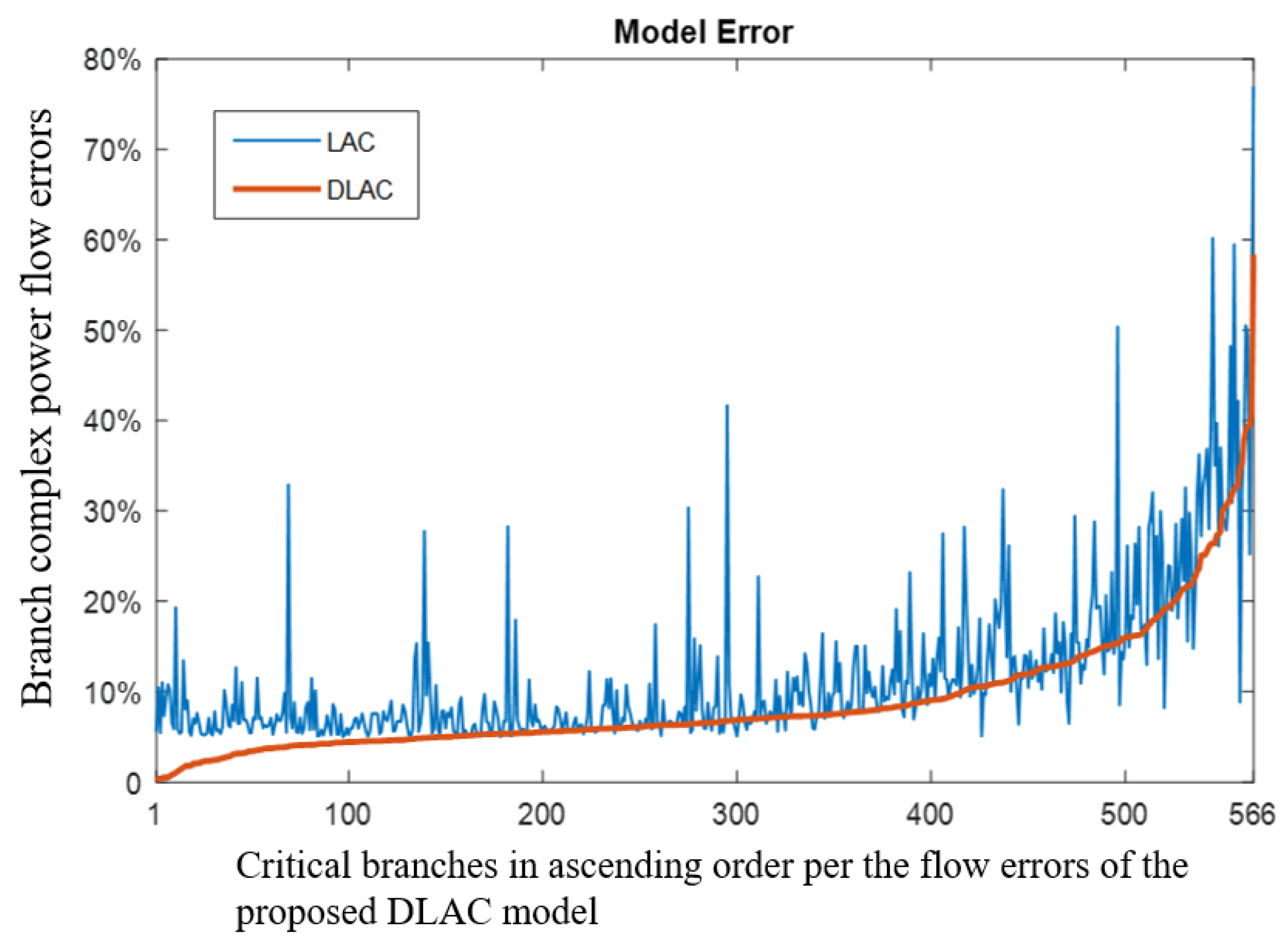
Two power flow simulations based on the regular LAC model and the proposed DLAC model are conducted on hour 1 case. As compared to the full AC model, the branch complex flow errors in percent for both LAC and DLAC are calculated and presented in Figure 4 where branches with less than 10 MVA flow and branches with flow errors less than 5% for LAC model are removed in order to clearly show the performance difference between the regular LAC model and the proposed DLAC model. There are 683 branches in Figure 4 and they are ordered based on flow errors of the proposed DLAC model. It is clearly observed from Figure 4 that the complex power flow errors of DLAC are well lower than LAC for most branches. To verify the proposed DLAC model on a different system operating condition, similar simulations are performed on hour 2 case representing the system scenario of the next following hour and the results are shown in Figure 5. Very similar observations can be made from Figure 5, which validates the proposed DLAC model. It is concluded the proposed DLAC model can substantially improve the regular LAC model with regression analysis.

With above analysis, it is demonstrated that the proposed data-driven linearized AC power flow model can largely enhance the system reactive power profile and voltage profile for the training case on which regression analysis is performed and the case of the very next following hour. Moreover, the proposed DLAC model and the traditional LAC model are tested on 70 more consecutive cases. The results are shown in

Table 14. Improvement of Voltage Magnitude for 72 Consecutive Cases.

Hour	LAC	DLAC	${\mathit{\eta }}_{\mathit{D}\mathit{L}\mathit{A}\mathit{C},\mathit{L}\mathit{A}\mathit{C}}$	Hour	LAC	DLAC	${\mathit{\eta }}_{\mathit{D}\mathit{L}\mathit{A}\mathit{C},\mathit{L}\mathit{A}\mathit{C}}$	Hour	LAC	DLAC	${\mathit{\eta }}_{\mathit{D}\mathit{L}\mathit{A}\mathit{C},\mathit{L}\mathit{A}\mathit{C}}$
1	0.0161	0.0105	35.0%	25	0.0169	0.0115	31.8%	49	0.0154	0.0098	36.0%
2	0.0153	0.0097	36.8%	26	0.0158	0.0104	34.3%	50	0.0145	0.0089	38.5%
3	0.0144	0.0085	41.2%	27	0.0137	0.0079	42.0%	51	0.0136	0.0076	43.8%
4	0.0116	0.0055	52.2%	28	0.0116	0.0056	51.4%	52	0.0116	0.0054	53.1%
5	0.0095	0.0034	63.8%	29	0.0102	0.0042	58.6%	53	0.0101	0.0039	61.3%
6	0.0089	0.0029	66.9%	30	0.0092	0.0034	63.6%	54	0.0093	0.0032	65.5%
7	0.0091	0.0032	65.2%	31	0.0091	0.0033	63.9%	55	0.0090	0.0030	66.7%
8	0.0090	0.0031	65.8%	32	0.0090	0.0031	65.2%	56	0.0088	0.0028	68.6%
9	0.0090	0.0029	67.3%	33	0.0089	0.0029	67.4%	57	0.0089	0.0027	69.8%
10	0.0088	0.0027	68.7%	34	0.0090	0.0030	66.5%	58	0.0090	0.0028	68.5%
11	0.0091	0.0030	67.1%	35	0.0092	0.0031	65.9%	59	0.0090	0.0027	69.6%
12	0.0105	0.0043	58.9%	36	0.0100	0.0039	61.1%	60	0.0094	0.0031	67.1%
13	0.0106	0.0044	58.2%	37	0.0105	0.0044	58.4%	61	0.0101	0.0038	62.7%
14	0.0117	0.0056	52.4%	38	0.0110	0.0050	54.8%	62	0.0108	0.0045	58.3%
15	0.0131	0.0070	46.3%	39	0.0119	0.0060	50.1%	63	0.0118	0.0055	52.9%
16	0.0144	0.0085	41.1%	40	0.0135	0.0076	43.4%	64	0.0144	0.0085	41.2%
17	0.0159	0.0101	36.9%	41	0.0145	0.0087	40.1%	65	0.0138	0.0078	43.7%
18	0.0163	0.0108	34.1%	42	0.0150	0.0095	37.1%	66	0.0148	0.0089	39.8%
19	0.0160	0.0107	33.0%	43	0.0157	0.0103	34.2%	67	0.0147	0.0091	38.1%
20	0.0185	0.0132	28.8%	44	0.0167	0.0114	31.8%	68	0.0150	0.0095	36.7%
21	0.0177	0.0125	29.4%	45	0.0174	0.0122	29.9%	69	0.0167	0.0112	33.1%
22	0.0179	0.0127	29.0%	46	0.0175	0.0123	29.6%	70	0.0171	0.0116	32.1%
23	0.0173	0.0121	30.3%	47	0.0165	0.0112	32.1%	71	0.0165	0.0110	33.4%
24	0.0160	0.0107	33.1%	48	0.0151	0.0097	35.6%	72	0.0159	0.0102	35.8%

and

Table 15. Improvement of Reactive Power for Branches Exceeding 10 MVAr for 72 Consecutive Cases.

Hour	LAC	DLAC	${\mathit{\eta }}_{\mathit{D}\mathit{L}\mathit{A}\mathit{C},\mathit{L}\mathit{A}\mathit{C}}$	Hour	LAC	DLAC	${\mathit{\eta }}_{\mathit{D}\mathit{L}\mathit{A}\mathit{C},\mathit{L}\mathit{A}\mathit{C}}$	Hour	LAC	DLAC	${\mathit{\eta }}_{\mathit{D}\mathit{L}\mathit{A}\mathit{C},\mathit{L}\mathit{A}\mathit{C}}$
1	36.0%	23.6%	34.5%	25	39.6%	27.0%	31.9%	49	37.0%	23.3%	37.2%
2	35.4%	22.8%	35.5%	26	39.6%	25.9%	34.6%	50	33.1%	20.7%	37.3%
3	33.6%	20.9%	37.8%	27	32.7%	19.7%	39.8%	51	31.3%	18.8%	40.1%
4	28.8%	16.8%	41.9%	28	27.0%	15.8%	41.6%	52	28.8%	16.7%	42.1%
5	22.2%	12.5%	43.6%	29	25.1%	14.2%	43.5%	53	25.6%	14.1%	44.8%
6	22.1%	12.2%	45.1%	30	23.1%	12.9%	44.0%	54	23.3%	13.0%	44.2%
7	22.5%	12.3%	45.4%	31	22.7%	12.9%	43.1%	55	22.7%	12.9%	43.4%
8	22.9%	12.6%	45.1%	32	22.1%	12.7%	42.6%	56	21.9%	12.3%	44.0%
9	23.0%	12.6%	45.0%	33	21.5%	12.2%	43.2%	57	21.2%	11.7%	44.8%
10	21.9%	12.4%	43.6%	34	21.7%	12.5%	42.3%	58	21.9%	12.3%	43.9%
11	22.9%	12.7%	44.6%	35	22.2%	12.6%	43.5%	59	21.7%	12.4%	42.9%
12	27.0%	14.9%	44.7%	36	23.4%	13.2%	43.5%	60	23.1%	13.0%	44.0%
13	28.2%	15.8%	43.8%	37	25.3%	14.3%	43.5%	61	23.5%	13.2%	43.8%
14	30.7%	18.0%	41.5%	38	26.6%	15.01%	43.5%	62	25.9%	14.5%	44.0%
15	35.1%	21.7%	38.1%	39	31.5%	18.7%	40.8%	63	27.3%	16.3%	40.2%
16	36.1%	22.5%	37.8%	40	35.4%	21.5%	39.3%	64	36.3%	22.6%	37.7%
17	38.4%	25.1%	34.6%	41	36.5%	22.6%	38.1%	65	34.4%	20.6%	40.2%
18	40.2%	26.5%	34.0%	42	35.9%	23.3%	35.1%	66	34.4%	21.6%	37.2%
19	39.7%	26.6%	33.0%	43	39.7%	26.0%	34.5%	67	35.8%	23.0%	35.7%
20	46.6%	32.3%	30.7%	44	39.8%	26.9%	32.5%	68	37.6%	23.2%	38.2%
21	44.1%	30.3%	31.3%	45	43.7%	30.1%	31.1%	69	38.9%	25.9%	33.2%
22	42.0%	29.1%	30.9%	46	42.1%	28.5%	32.3%	70	40.1%	27.2%	32.2%
23	40.8%	27.9%	31.5%	47	38.1%	25.7%	32.6%	71	38.9%	25.9%	33.3%
24	39.1%	26.0%	33.6%	48	36.9%	23.5%	36.5%	72	40.5%	25.8%	36.3%

.

The average voltage improvement with the proposed DLAC model against the regular LAC model over all 72 cases has a mean of 48.7% and a standard deviation of 14.2%; the average branch reactive power improvement with DLAC against LAC is 39.8% with a standard deviation of 4.7%. This demonstrates the proposed DLAC power flow model significantly improve the regular LAC model. The average error of voltage solutions obtained from DLAC is only 0.67% among 72 system scenarios. The standard deviation of voltage error is 0.33%, which indicates the proposed DLAC model is stable and robust over different system conditions. For branch reactive power, the average error is 19.4% with a standard deviation of 6%, and although reactive power solution is not as accurate as voltage, the proposed DLAC can provide reactive power information within an acceptable range, which shows its superiority over the traditional DC power flow model.

It is worth noting that determining regressors’ coefficients with linear regression is fast and the regression model can be easily retrained with the latest system operating data. However, frequent model retraining may not be necessary unless the system voltage profile and operating points have significantly deviated from the previous training data. This feature can enable the proposed DLAC model to be integrated in several power system applications, such as economic dispatch, unit commitment, and grid expansion planning.

6. Conclusions

Due to nonlinearity and nonconvexity of the AC power flow model, the simplified DC model is widely used in both academic and industry. However, the DC power flow model does not include any information about reactive power and voltage profile. To maintain linearity while capturing reactive power and voltage, this work first introduced a regular LAC model and then proposed a data-driven enhanced LAC model. The proposed DLAC model can improve the regular LAC model by tuning the coefficients with the regression analysis technology. Both regular LAC and enhanced DLAC model can substantially reduce the error associated with calculated branch active power flows against the traditional DC power flow model. Moreover, as compared with the regular LAC model, the proposed DLAC model can obtain a more accurate voltage profile and improve reactive power flow solutions. The reason why DLAC model is more accurate is that the enhanced DLAC model can take recent/historical system conditions into account. It is worth noting that the proposed DLAC model can be easily incorporated in various power system applications such as day-ahead unit commitment or real-time economic dispatch, which can substantially improve their performance.

Case studies on the large-scale practical TVA system demonstrate the performance and effectiveness of the proposed DLAC model. Numerical simulations show that the proposed DLAC model can substantially improve the reactive power and voltage solutions against the regular LAC model. The simulation results also show that there is no overfitting or multicollinearity issue for the proposed DLAC model, which indicates that the proposed DLAC model is robust.

References

- Wang, G.; Zamzam, A.S.; Giannakis, G.B.; Sidiropoulos, N.D. Power system state estimation via feasible point pursuit: Algorithms and Cramér-Rao bound. IEEE Trans. Signal Process. 2018, 66, 1649–1658. [Google Scholar] [CrossRef]
- Zhao, J.; Gómez-Expósito, A.; Netto, M.; Mili, L.; Abur, A.; Terzija, V.; Kamwa, I.; Pal, B.; Singh, A.K.; Qi, J.; et al. Power system dynamic state estimation: Motivations, definitions, methodologies, and future work. IEEE Trans. Power Syst. 2019, 34, 3188–3198. [Google Scholar] [CrossRef]
- Li, X.; Hedman, K.W. Enhanced energy management system with corrective transmission switching strategy—Part I: Methodology. IEEE Trans. Power Syst. 2019, 34, 4490–4502. [Google Scholar] [CrossRef] [Green Version]
- Li, X.; Hedman, K.W. Enhanced energy management system with corrective transmission switching strategy—Part II: Results and discussion. IEEE Trans. Power Syst. 2019, 34, 4503–4513. [Google Scholar] [CrossRef] [Green Version]
- Li, X.; Xia, Q. Stochastic optimal power flow with network reconfiguration: Congestion management and facilitating grid integration of renewables. In Proceedings of the IEEE PES T&D Conference & Exposition, Chicago, IL, USA, 12–15 October 2020. [Google Scholar]
- Ramesh, A.V.; Li, X. Security-constrained unit commitment with corrective transmission switching. In Proceedings of the North American Power Symposium (NAPS), Wichita, KS, USA, 13–15 October 2019. [Google Scholar]
- Ramesh, A.V.; Li, X. Reducing congestion-induced renewable curtailment with corrective network reconfiguration in day-ahead scheduling. In Proceedings of the IEEE PES General Meeting, Montreal, QC, Canada, 3–6 August 2020. [Google Scholar]
- Li, X.; Hedman, K.W. Fast heuristics for transmission outage coordination. In Proceedings of the Power Systems Computation Conference (PSCC), Genoa, Italy, 20–24 June 2016. [Google Scholar]
- Li, X.; Xia, Q. Power system expansion planning with seasonal network optimization. In Proceedings of the Innovative Smart Grid Technologies (ISGT), Washington, DC, USA, 17–20 February 2020. [Google Scholar]
- Kwon, J.; Hedman, K.W. Transmission expansion planning model considering conductor thermal dynamics and high temperature low sag conductors. IET Gener. Transm. Distrib. 2015, 9, 2311–2318. [Google Scholar] [CrossRef]
- Kwon, J.; Zhi, Z.; Levin, T.; Botterud, A. A stochastic multi-agent resource planning model: The impact of capacity remuneration mechanisms. In Proceedings of the IEEE International Conference on Probabilistic Methods Applied to Power Systems (PMAPS), Boise, ID, USA, 24–28 June 2018. [Google Scholar]
- Kwon, J.; Zhou, Z.; Levin, T.; Botterud, A. Resource adequacy in electricity markets with renewable energy. IEEE Trans. Power Syst. 2020, 35, 773–781. [Google Scholar] [CrossRef]
- Zhang, Y.S.; Chiang, H.D. Fast Newton-FGMRES solver for large-scale power flow study. IEEE Trans. Power Syst. 2010, 25, 769–776. [Google Scholar] [CrossRef]
- Pirnia, M.; Cañizares, C.A.; Bhattacharya, K. Revisiting the power flow problem based on a mixed complementarity formulation approach. IET Gener. Transm. Distrib. 2013, 7, 1194–1201. [Google Scholar] [CrossRef]
- Carpentier, J. Contribution to the economic dispatch problem. Bull. Soc. Fr. Electr. 1962, 3, 431–447. (In French) [Google Scholar]
- Bent, R.; Coffrin, C.; Gumucio, R.R.E.; Van Hentenryck, P. Transmission network expansion planning: Bridging the gap between AC heuristics and DC approximations. In Proceedings of the Power Systems Computation Conference, Wroclaw, Poland, 18–22 August 2014. [Google Scholar]
- Phillipe Vilaça, G.; Tomé Saraiva, J. A two-stage strategy for security-constrained AC dynamic transmission expansion planning. Electr. Power Syst. Res. 2020, 180, 106167. [Google Scholar]
- Villanueva, D.; Feijóo, A.E.; Pazos, J.L. An analytical method to solve the probabilistic load flow considering load demand correlation using the DC load flow. Electr. Power Syst. Res. 2014, 110, 1–8. [Google Scholar] [CrossRef]
- Cheng, X.; Overbye, T.J. PTDF-based power system equivalents. IEEE Trans. Power Syst. 2005, 20, 1868–1876. [Google Scholar] [CrossRef]
- Stott, B.; Jardim, J.; Alsaç, O. DC power flow revisited. IEEE Trans. Power Syst. 2009, 24, 1290–1300. [Google Scholar] [CrossRef]
- Yan, J.; Tang, Y.; He, H.; Sun, Y. Cascading failure analysis with DC power flow model and transient stability analysis. IEEE Trans. Power Syst. 2015, 30, 285–297. [Google Scholar] [CrossRef]
- Purchala, K.; Meeus, L.; Dommelen, D.V.; Belmans, R. Usefulness of DC power flow for active power flow analysis. In Proceedings of the IEEE PES General Meeting, San Francisco, CA, USA, 12–16 June 2005. [Google Scholar]
- Qi, Y.; Shi, D.; Tylavsky, D. Impact of assumptions on DC power flow model accuracy. In Proceedings of the North American Power Symposium (NAPS), Champaign, IL, USA, 9–11 September 2012. [Google Scholar]
- Coffrin, C.; Hentenryck, P.V. A linear-programming approximation of AC power flows. INFORMS J. Comput. 2014, 26, 718–734. [Google Scholar] [CrossRef]
- Koster, A.M.; Lemkens, S. Designing AC power grids using integer linear programming. In Network Optimization; Springer: Berlin/Heidelberg, Germany, 2011; pp. 478–483. [Google Scholar]
- Taylor, J.A.; Hover, F.S. Linear relaxations for transmission system planning. IEEE Trans. Power Syst. 2011, 26, 2533–2538. [Google Scholar] [CrossRef] [Green Version]
- Peterson, N.M.; Tinney, W.F.; Bree, D.W., Jr. Iterative linear AC power flow solution for fast approximate outage studies. IEEE Trans. Power Appar. Syst. 1972, 2048–2056. [Google Scholar] [CrossRef]
- Allen, J.; Wollenberg, B.F.; Sheblé, G.B. Power Generation, Operation, and Control, 3rd ed.; John Wiley & Sons: Hoboken, NJ, USA, 2013; ISBN 978-0-471-79055-6. [Google Scholar]
- Yan, X.; Su, X. Linear Regression Analysis: Theory and Computing, 1st ed.; World Scientific: Singapore, 2009; ISBN -13: 978-9812834102. [Google Scholar]
- Montgomery, D.C.; Peck, E.A.; Vining, G.G. Introduction to Linear Regression Analysis, 5th ed.; John Wiley & Sons: Hoboken, NJ, USA, 2012; Volume 821. [Google Scholar]
- Kraiczy, N. Innovations in Small and Medium-Sized Family Firms: An Analysis of Innovation Related Top Management Team Behaviors and Family Firm-Specific Characteristics; Springer Science & Business Media: Berlin, Germany, 2013; ISBN 978-3-658-00063-9. [Google Scholar]
- Zhang, H.; Heydt, G.T.; Vittal, V.; Quintero, J. An improved network model for transmission expansion planning considering reactive power and network losses. IEEE Trans. Power Syst. 2018, 28, 3471–3479. [Google Scholar] [CrossRef]
- Liu, Y.; Zhang, N.; Wang, Y.; Yang, J.; Kang, C. Data-driven power flow linearization: A regression approach. IEEE Trans. Smart Grid 2019, 10, 2569–2580. [Google Scholar] [CrossRef] [Green Version]
- Tan, Y.; Chen, Y.; Li, Y.; Cao, Y. Linearizing power flow model: A hybrid physical model-driven and data-driven approach. IEEE Trans. Power Syst. 2020, 35, 2475–2478. [Google Scholar] [CrossRef]
- Tennessee Valley Authority, Federally Owned Corporation in the United States. Available online: https://www.tva.gov/ (accessed on 20 June 2020).
- Li, X.; Balasubramanian, P.; Abdi-Khorsand, M.; Korad, A.S.; Hedman, K.W. Effect of topology control on system reliability: TVA test case. In Proceedings of the CIGRE US National Committee Grid of the Future Symposium, Houston, TX, USA, 20 October 2014. [Google Scholar]
- R Core Team. R: A Language and Environment for Statistical Computing; R Foundation for Statistical Computing: Vienna, Austria, 2018. Available online: https://www.R-project.org/ (accessed on 20 June 2020).
Figure 1.
Single-line diagram of a 2-terminal circuit.
Figure 2.
Plots of residuals against fitted values of branch power for hour 1 case: (a) Original residual e versus fitted value; (b) Standardized residual d versus fitted value; (c) R-student residual t versus fitted value.
Figure 3.
Branch flows of fitted DLAC model versus AC model for hour 1 case.
Figure 4.
Branch complex power flow errors of LAC model and DLAC model for hour 1 case.
Figure 5.
Branch complex power flow errors of LAC model and DLAC model for hour 2 case.