Thermodynamic Optimization of a Waste Heat Power System under Economic Constraint

Abstract

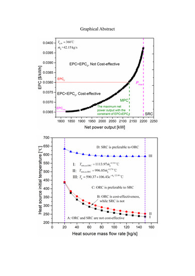
A novel thermo-economic performance indicator for a waste heat power system, namely, MPC, is proposed in this study, which denotes the maximum net power output with the constraint of EPC ≤ EPC₀, where EPC is the electricity production cost of the system and EPC₀ refers to the EPC of conventional fossil fuel power plants. The organic and steam Rankine cycle (ORC, SRC) systems driven by the flue gas are optimized to maximize the net power output with the constraint of EPC ≤ EPC₀ by using the Non-dominated Sorting Genetic Algorithm-II (NSGA-II). The optimization process entails the design of the heat exchangers, the instantaneous calculation of the turbine efficiency, and the system cost estimation based on the Aspen Process Economic Analyzer. Six organic fluids, n-butane, R245fa, n-pentane, cyclo-pentane, MM (Hexamethyldisiloxane), and toluene, are considered for the ORC system. Results indicate that the MPC of the ORC system using cyclo-pentane is 39.7% higher than that of the SRC system under the waste heat source from a cement plant with an initial temperature of 360 °C and mass flow rate of 42.15 kg/s. The precondition of the application of the waste heat power system is EPC ≤ EPC₀, and the minimum heat source temperatures to satisfy this condition for ORC and SRC systems are obtained. Finally, the selection map of ORC versus SRC based on their thermo-economic performance in terms of the heat source conditions is provided.

1. Introduction

Large quantities of waste heat are generated during the working processes of internal combustion engines, gas turbines, and many industries [1,2]. Recovering the waste heat helps reduce fossil energy consumption and the related emissions of CO₂ and atmospheric pollutants. One of the feasible ways is to convert the waste heat to electricity via power cycle systems.

Flue gas waste heat is generally discharged to the environment after heat release from the system; hence, we intend to recover as much electricity from the flue gas as possible. On the other hand, we also want to reduce the electricity production cost (EPC) of the waste heat power system, since the cost actually represents the energy and material resources consumed by the system from its manufacturing to operation and maintenance. In other words, the EPC reveals the utilization efficiency of the total energy and material resources of the system.

However, in some cases, the two objectives are in conflict. For example, given the waste heat source condition, the system’s net power output and EPC under two different design schemes are as follows: (A) 2.4 MW, 0.034 $/kWh, (B) 3.5 MW, 0.044 $/kWh. Plan A shows a lower EPC, but the electricity recovered from the heat source is also significantly lower than that of plan B. Therefore, which solution should we choose to design the system?

Here, we introduce the electricity production cost of a conventional fossil fuel power system, EPC₀, as a benchmark value. If the EPC of the waste heat power system is higher than EPC₀, it means that the waste heat power system consumes more energy and resources per unit of power generation than that of the fossil fuel power system, indicating that the waste heat power system cannot achieve energy saving. Therefore, the precondition of the application of the waste heat power system is EPC ≤ EPC₀. Only if this condition is satisfied can the system be cost-effective.

Based on this, we propose that the thermo-economic optimization objective of the waste heat power system is to maximize the net power output with the constraint of EPC ≤ EPC₀. For convenience, the maximum net power output with the constraint of EPC ≤ EPC₀ of the system is abbreviated as MPC.

The Rankine Cycle (RC) with water as the working fluid, namely, the steam Rankine cycle (SRC), is the conventional technology in waste heat power systems [3], while the organic Rankine cycle (ORC) has attracted more attention in the past few years due to the low to moderate temperature sources [4]. Comparative studies of ORC and SRC mostly focused on the thermodynamic performance. Karellas et al. [5] compared the energy and exergy efficiencies of the SRC and isopentane-RC systems. Results proved that the SRC achieves the better performance when the initial temperature of the exhaust gas exceeds 310 °C. Andreasen et al. [6] investigated the dual pressure SRC and the ORC for waste heat recovery from a marine engine. The results indicated that the net power output of the SRC system was higher at high engine loads, and the ORC system produced more power at lower engine loads. Santiago et al. [7] demonstrated that the ORC outperforms the SRC across the whole engine loading range. Li and Wang [8] optimized the net power output of ORC, SRC, and some other power cycles for waste heat recovery under different heat source conditions. The results indicated that SRC showed the poorest performance at an initial flue gas temperature lower than 500 °C.

This study aims to compare the MPC of the ORC and SRC systems for waste heat recovery and obtain the selection map that enables a straightforward selection between the two systems in terms of the heat source conditions. Hence, ORC and SRC systems are optimized to maximize the net power output with the constraint of EPC ≤ EPC_0, and the decision variables are evaporating temperature, turbine inlet temperature, condensing temperature, pinch point temperature difference in HRSG (heat recovery steam generator), and regenerator effectiveness (for ORC only). The relevant research methods including the heat exchanger design, turbine efficiency calculation, and system cost estimation are established. The GA (genetic algorithm) and NSGA-II (non-dominated sorting genetic algorithm) are employed as the optimization algorithms. Figure 1 shows the thermo-economic optimization process of the two systems.

2. System Description

The basic ORC and SRC systems have the same components: heat recovery steam generator (HRSG), turbine, power generator, condenser, working fluid pump, cooling water pump, and cooling tower. If the organic fluid is “too dry”, the turbine exhaust temperature is higher than the condensing temperature and introducing a regenerator can improve the thermal efficiency of the ORC system. Figure 2 shows the T–s diagrams of the regenerative ORC and SRC.

Figure 3 shows the schematic diagram of the regenerative ORC system for waste heat recovery. The working fluid coming from the condenser is compressed to the evaporating pressure by the pump (4–5), and then it is heated in the regenerator (5–6) before flowing into HRSG. In the HRSG, the working fluid is preheated in the economizer, evaporates in the evaporator, and then becomes superheated vapor in the superheater by absorbing heat from the flue gas (6–1). The generated vapor expands in the turbine to do work (1–2). The turbine exhaust is delivered to the regenerator to heat the working fluid from the pump (2–3). Finally, the working fluid is condensed into the saturated liquid by the cooling water in the condenser (3–4) and then enters the working fluid pump to complete the cycle. For the SRC system, the steam at the turbine outlet is in a two-phase state, and it runs directly to the condenser.

3. Methodology

3.1. Thermodynamic and Economic Modeling

The energy analysis of the ORC and SRC systems is based on the first law of thermodynamics. Each component is considered as a steady-flow device and does not radiate heat to the environment. The change of the potential and kinetic energies and the pressure drop of working fluid in the system are neglected. The thermodynamic model of each component is as follows.

The heat transferred in the HRSG and condenser for the SRC system is evaluated by:

$${\dot{Q}}_{\mathrm{HRSG}}={\dot{m}}_{\mathrm{g}}{c}_{\mathrm{p},\mathrm{g}}\left(T_{\mathrm{g},\mathrm{in}}-T_{\mathrm{g},\mathrm{out}}\right)={\dot{m}}_{\mathrm{wf}}\left(h_1-h_5\right)$$

(1)

$${\dot{Q}}_{\mathrm{con}}={\dot{m}}_{\mathrm{water}}\left(h_{\mathrm{water},\mathrm{out}}-h_{\mathrm{water},\mathrm{in}}\right)={\dot{m}}_{\mathrm{wf}}\left(h_2-h_4\right)$$

(2)

The heat transferred in the HRSG, condenser, and regenerator for the regenerative ORC system is evaluated by:

$${\dot{Q}}_{\mathrm{HRSG}}={\dot{m}}_{\mathrm{g}}{c}_{\mathrm{p},\mathrm{g}}\left(T_{\mathrm{g},\mathrm{in}}-T_{\mathrm{g},\mathrm{out}}\right)={\dot{m}}_{\mathrm{wf}}\left(h_1-h_6\right)$$

(3)

$${\dot{Q}}_{\mathrm{con}}={\dot{m}}_{\mathrm{water}}\left(h_{\mathrm{water},\mathrm{out}}-h_{\mathrm{water},\mathrm{in}}\right)={\dot{m}}_{\mathrm{wf}}\left(h_3-h_4\right)$$

(4)

$${\dot{Q}}_{\mathrm{reg}}={\dot{m}}_{\mathrm{wf}}\left(h_2-h_3\right)={\dot{m}}_{\mathrm{wf}}\left(h_6-h_5\right)$$

(5)

The effectiveness of the regenerator is expressed as:

$${\epsilon }_{\mathrm{reg}}=\left(h_2-h_3\right)/\left(h_2-h_{\left({\mathrm{P}}_3,{\mathrm{T}}_3={\mathrm{T}}_5\right)}\right)$$

(6)

$h_{\left({\mathrm{P}}_3,{\mathrm{T}}_3={\mathrm{T}}_5\right)}$ refers to the enthalpy value of state point 3 assuming that its temperature is equal to that of state point 5.

The power output of the turbine is evaluated by:

$${\dot{W}}_{\mathrm{turb}}={\dot{m}}_{\mathrm{wf}}\left(h_1-h_2\right)={\dot{m}}_{\mathrm{wf}}\left(h_1-h_{2\mathrm{s}}\right){\eta }_{\mathrm{turb}}$$

(7)

The power input of the working fluid pump is evaluated by:

$${\dot{W}}_{\mathrm{pump},\mathrm{wf}}={\dot{m}}_{\mathrm{wf}}\left(h_5-h_4\right)={\dot{m}}_{\mathrm{wf}}\left(h_{5s}-h_4\right)/{\eta }_{\mathrm{pump},\mathrm{wf}}$$

(8)

The power input of the cooling water pump is determined by the flow rate and the pressure drop of the cooling water in the cooling loop:

$${\dot{W}}_{\mathrm{pump},\mathrm{water}}={\dot{m}}_{\mathrm{water}}\mathsf{\Delta }{P}_{\mathrm{water}}/\left({\rho }_{\mathrm{water}}{\eta }_{\mathrm{pump},\mathrm{water}}\right)$$

(9)

The net power output of the system is evaluated by:

$${\dot{W}}_{\mathrm{net}}={\dot{W}}_{\mathrm{turb}}-{\dot{W}}_{\mathrm{pump},\mathrm{wf}}-{\dot{W}}_{\mathrm{pump},\mathrm{water}}$$

(10)

The EPC of the system is calculated as [9]:

$$EPC=\frac{\left(CRF\cdot C_{\mathrm{system}}+C_{\mathrm{O}\text{\&}\mathrm{M}}\right)}{\left({\dot{W}}_{\mathrm{net}}\cdot t_{\mathrm{full}\mathrm{load}}\right)}$$

(11)

where $C_{\mathrm{system}}$ refers to the total cost of designing, constructing, and installing the waste heat power system. $C_{\mathrm{O}\text{\&}\mathrm{M}}$ is the operation and maintenance cost of the system and is set as 1.5% of the $C_{\mathrm{system}}$. $t_{\mathrm{full}\mathrm{load}}$ is the annual full-load operation time of the system and is set as 7500 h. CRF denotes the capital recovery factor, which is estimated by:

$$CRF=i\cdot \frac{{(1+i)}^{L{T}_{\mathrm{plant}}}}{{(1+i)}^{L{T}_{\mathrm{plant}}}-1}$$

(12)

The interest rate i and plant lifetime $L{T}_{\mathrm{plant}}$ are set as 5% and 20 years, respectively.

3.2. Turbine Efficiency Estimation

Considering the turbine efficiency varies with the operating parameters, the optimization process couples with the turbine efficiency estimation, which means the turbine efficiency is calculated instantaneously based on the given operating parameters.

The multi-stage axial flow turbine is an inevitable choice for the SRC system owing to the high specific enthalpy drop and volume ratio during the expansion process of the steam. The efficiency of the steam turbine is inherently limited for the low power applications since the small mass flow rate of the steam results in small flow passages, which will increase the friction and clearance losses. Bahadori and Vuthaluru [10] developed a practical, reliable, and easy-to-use method to estimate the steam turbine efficiency, which is determined by the turbine rating power and speed, steam inlet superheats and pressure, turbine load factor, and the number of stages. In the present study, the load factor and the number of stages of the steam turbine are taken as 100% and 11, respectively.

Considering the system capacity is of MW scale in this study, the ORC system also adopts an axial-flow turbine. The lower enthalpy drops during the expansion process of organic fluids (typically 10–100 kJ/kg) permit the turbine with a reduced number of stages and enable a high efficiency turbine design due to the adequately large flow passages. Macchi [11] indicated that the efficiency of the organic-axial flow turbine is determined by three variables: the size parameter (SP), the volume ratio (Vr), and the specific speed (Ns):

$$\begin{array}{c}Vr=\frac{V_{\mathrm{out},\mathrm{is}}}{V_{\mathrm{in}}}\\ SP=\frac{V_{\mathrm{out},\mathrm{is}}^{0.5}}{\mathsf{\Delta }{h}_{\mathrm{is}}^{0.25}}\\ Ns=\frac{RPM}{60}\frac{V_{\mathrm{out},\mathrm{is}}^{0.5}}{\mathsf{\Delta }{h}_{\mathrm{is}}^{0.75}}\end{array}$$

(13)

For a given SP and Vr, there exists an optimal Ns whose value is generally 0.1–0.15 to maximize the turbine efficiency. A small SP causes large leakage and secondary losses, resulting in a sharp efficiency drop. Organics generally have a large molar mass, which entails a lower sound speed. Hence, the multistage turbine should be considered when the Vr is higher than 4 to avoid a high Mach number [12]. A multistage turbine can achieve higher efficiency, but also increases the component complexity and cost. In the present study, a three-stage turbine is considered for the ORC system. Its efficiency is estimated based on Equation (14), and the numerical values of the retrieved coefficient are listed in

Table 1. Regressed coefficients to be used in Equation (14) [11].

i	Fi	Ai	i	Fi	Ai
0	1	0.932274	7	ln(Vr)4	0.000298
1	ln(SP)	−0.01243	8	ln(Vr) ln(SP)	0.005959
2	ln(SP)2	−0.018	9	ln(Vr)2 ln(SP)	−0.00163
3	ln(SP)3	−0.00716	10	ln(Vr) ln(SP)2	0.001946
4	ln(SP)4	−0.00118	11	ln(Vr)3 ln(SP)	0.000163
5	Vr	−0.00044	12	ln(Vr)2 ln(SP)3	0.000211
6	ln(Vr)3	−0.0016	−	−	−

[11].

$${\eta }_{\mathrm{turb}}={\displaystyle \sum }_{i=0}^{12}{A}_{\mathrm{i}}{F}_{\mathrm{i}}$$

(14)

3.3. Heat Exchanger Design

The cost of heat exchangers contributes largely to the total system cost. It is crucial to select a suitable heat exchanger configuration considering the working condition and the properties of the heat exchanging fluids. The flue gas has a poor heat transfer performance and may contain fly ash and dust. Thus, the finned tube waste heat boiler is adopted as the HRSG. The shell-and-tube heat exchanger is adopted as the condenser. The considered regenerator is a plate-fin heat exchanger due to its high heat transfer efficiency and compact structure.

3.3.1. Heat Recovery Steam Generator

The working fluid flows in the tube, and the flue gas flows across the tube bundles. The heat transfer coefficient of the flue gas is much lower than that of the working fluid; thus, the annular fin-tube is used to reduce the thermal resistance of the flue gas side. The parameters of the HRSG are given in

Table 2. Parameters and restrictions of the heat exchangers.

HRSG		Condenser
Tube outside diameter, do (mm)	38	Tube outside diameter, do (mm)		18
Tube inside diameter, di (mm)	31	Tube inside diameter, di (mm)		15
Tube pitch, Pt (mm)	80	Inlet velocity of cooling water, (m/s)		1.5
Fin height, H (mm)	15	Inlet velocity of working fluid, (m/s)		40
Fin thickness, t (mm)	1	Fouling factor of cooling water, (m2·K/W)		0.0003
Fin spacing, Y (mm)	5	Shell and tube material		CS
Allowable pressure drops in tube, (kPa)	150	Plate-fin Regenerator
Allowable pressure drops in shell, (Pa)	1000		Vapor Side	Liquid Side
Tube wall thermal conductivity (W/m·K)	45	Fin height, H (mm)	9.5	4.7
Fouling factor of flue gas, (m2·K/W)	0.0005	Fin thickness, $\delta$ (mm)	0.2	0.3
Fouling factor of organic, (m2·K/W)	0.0002	Plate thickness, $\delta ’$ (mm)	0.2	0.3
Fouling factor of cooling water, (m2·K/W)	0.0002	Fin spacing, S (mm)	1.7	2.0
Tube and fin material	CS	Plate wide, B (mm)	720	720
		Plate and fin material	Aluminum

.

As depicted in Figure 4, the heat addition process of the working fluid in the HRSG consists of three parts: preheating, evaporating, and superheating. The heat exchange area of the HRSG is the sum of the three sections.

The outside surface area of the heat transfer tubes for each region is evaluated as:

$$A=\frac{\dot{Q}}{KF\mathsf{\Delta }{T}_{\mathrm{lm}}}$$

(15)

where $\dot{Q}$ is the total heat transfer rate in each region, K refers to the overall heat transfer coefficient based on the outside surface of bare tubes. $\mathsf{\Delta }{T}_{\mathrm{lm}}$ denotes the logarithmic mean temperature difference (LMTD) between the flue gas and working fluid. F is the correction factor of the LMTD since the flow between the flue gas and working fluid is not rigorous countercurrent, and it can be computed as described in Ref. Bowman [13].

$$K={\left[\left(\frac{1}{h_{\mathrm{i}}}+R_{\mathrm{f},\mathrm{i}}\right)\frac{d_{\mathrm{o}}}{d_{\mathrm{i}}}+\frac{d_{\mathrm{o}}}{2\lambda }\ln \left(\frac{d_{\mathrm{o}}}{d_{\mathrm{i}}}\right)+\left(\frac{1}{h_{\mathrm{o}}}+R_{\mathrm{f},\mathrm{o}}\right)\frac{1}{{\eta }_{\mathrm{o}}\beta }\right]}^{-1}$$

(16)

where $h_{\mathrm{i}}$ and $h_{\mathrm{o}}$ are the heat transfer coefficients of the respective working fluid and flue gas. $R_{\mathrm{f},\mathrm{i}}$ and $R_{\mathrm{f},\mathrm{o}}$ are the corresponding fouling factors. $\lambda$ refers to the thermal conductivity of the tube wall. ${\eta }_{\mathrm{o}}$ is the overall fin surface efficiency, and $\beta$ is the finned ratio.

$$\begin{array}{c}{\eta }_0=\frac{{\eta }_{\mathrm{f}}{A}_{\mathrm{f}}+A_{\mathrm{b}}}{A_{\mathrm{f}}+A_{\mathrm{b}}}\\ \beta =\frac{A_{\mathrm{f}}+A_{\mathrm{b}}}{A_{\mathrm{i}}}\end{array}$$

(17)

where $A_{\mathrm{f}}$ and $A_{\mathrm{b}}$ are the surface area of fins and the bare region outside the tubes, respectively, and $A_{\mathrm{i}}$ is the inside area of the tubes. For the annular fins, the calculation of the fin efficiency ${\eta }_{\mathrm{f}}$ can be simplified as follows [14]:

$$\begin{array}{c}{\eta }_{\mathrm{f}}=\frac{\tanh (ml)}{ml}\\ ml=\left(H+\frac{t}{2}\right)\sqrt{\frac{2h_{\mathrm{o}}}{\lambda t}}\sqrt{1+\frac{H}{d_{\mathrm{o}}}}\end{array}$$

(18)

(a)

Flue gas side

The heat transfer coefficient and pressure drop of the flue gas flowing across the staggered tube bundles can be obtained by the Briggs–Young correlations [15]:

$$h_{\mathrm{o}}=0.1378\left(\frac{{\lambda }_{\mathrm{g}}}{d_{\mathrm{o}}}\right){\left(\frac{d_{\mathrm{o}}{G}_{\mathrm{m},\mathrm{g}}}{{\mu }_{\mathrm{g}}}\right)}^{0.718}P{r}_{\mathrm{g}}^{0.33}{\left(\frac{Y}{H}\right)}^{0.296}$$

(19)

$$\begin{array}{c}\mathsf{\Delta }{P}_{\mathrm{g}}=f\cdot \frac{N_{\mathrm{tube}}{G}_{\mathrm{m},\mathrm{g}}^2}{2{\rho }_{\mathrm{g}}}\\ f=37.86{\left(\frac{d_{\mathrm{o}}{G}_{\mathrm{m},\mathrm{g}}}{{\mu }_{\mathrm{g}}}\right)}^{0.718}{\left(\frac{P_{\mathrm{t}}}{d_{\mathrm{o}}}\right)}^{-0.927}\end{array}$$

(20)

where $G_{\mathrm{m},\mathrm{g}}$ is the mass flux of the flue gas and $N_{\mathrm{tube}}$ refers to the number of the tube rows.

(b)

Working fluid side–single-phase region

The heat transfer coefficient of the single-phase working fluid flowing in the horizontal tube can be obtained by the Petukhov correlation [16]:

$$\begin{array}{c}{h}_{\mathrm{i}}=\frac{{\lambda }_{\mathrm{wf}}}{d_{\mathrm{i}}}\cdot \frac{\left(f/8\right)R{e}_{\mathrm{wf}}P{r}_{\mathrm{wf}}}{12.7{\left(f/8\right)}^{0.5}\left(P{r}_{\mathrm{wf}}^{2/3}-1\right)+1.07}\\ f={\left(1.82\cdot lg\left(R{e}_{\mathrm{wf}}\right)-1.64\right)}^{-2}\end{array}$$

(21)

The total pressure drops of the single-phase working fluid flowing in the HRSG can be calculated by [15]:

$$\begin{array}{c}\mathsf{\Delta }{P}_{\mathrm{wf}}=0.5{\rho }_{\mathrm{wf}}{u}_{\mathrm{wf}}^2\left[f_{\mathrm{wf}}{N}_{\mathrm{tube}}{L}_{\mathrm{tube}}/d_{\mathrm{i}}+3N_{\mathrm{tube}}+1.5\right]\\ f_{\mathrm{wf}}=64/R{e}_{\mathrm{wf}},R{e}_{\mathrm{wf}}<2000\\ f_{\mathrm{wf}}=0.3164/R{e}_{\mathrm{wf}}^{0.25},R{e}_{\mathrm{wf}}>2000\end{array}$$

(22)

(c)

Working fluid side–two-phase region

The Kandlikar semi-empirical correlation [17] is selected to estimate the heat transfer coefficient for the working fluid evaporating in the horizontal tube:

$$\begin{array}{c}{h}_i=h_L\cdot \left[C_{1}C{o}^A{\left(25F{r}_{\mathrm{L}}\right)}^B+C_{2}B{o}^C{F}_{\mathrm{L}}\right]\\ A=-0.9,B=0.3,C=0.7,C_1=1.136,C_2=667.2,Co\le 0.65\\ A=-0.2,B=0.3,C=0.7,C_1=0.6683,C_2=1058,Co>0.65\end{array}$$

(23)

$$h_{\mathrm{L}}=\frac{{\lambda }_{\mathrm{L}}}{d_{\mathrm{i}}}\cdot 0.023\cdot {\left[\frac{G_{\mathrm{wf}}(1-x)d_{\mathrm{i}}}{{\mu }_{\mathrm{L}}}\right]}^{0.8}P{r}_{\mathrm{L}}^{0.4}$$

(24)

The convective boiling number $Co$, nucleate boiling number $Bo$, and liquid Froude number $F{r}_{\mathrm{L}}$ are calculated by the following equations:

$$Co={\left(\frac{1-x}{x}\right)}^{0.8}{\left(\frac{{\rho }_{\mathrm{g}}}{{\rho }_{\mathrm{L}}}\right)}^{0.8}Bo=\frac{q}{G_{\mathrm{wf}}\mathsf{\Delta }{H}_{\mathrm{vap}}}F{r}_l=\frac{G_{\mathrm{wf}}^2}{9.8{\rho }_{\mathrm{L}}^2{d}_{\mathrm{i}}}$$

(25)

$x$ denotes the vapor quality and q is the heat flux. The evaporating zone is divided into 100 segments with an identical heat transfer rate, and the total area of the evaporating section is the sum of each segment.

The pressure drops of the working fluid evaporating inside the tubes are due to the friction and acceleration, and the latter reflects the change in flow kinetic energy. The total pressure drops can be evaluated as follows:

$$\mathsf{\Delta }{P}_{\mathrm{wf}}=\mathsf{\Delta }{P}_{\mathrm{acc}}+\mathsf{\Delta }{P}_{\mathrm{fric}}$$

(26)

The acceleration pressure drop is obtained by [18]:

$$\mathsf{\Delta }{P}_{\mathrm{acc}}=G_{\mathrm{wf}}^2\left\{\left[\frac{x_{\mathrm{o}}^2}{{\rho }_{\mathrm{v}}{\alpha }_{\mathrm{o}}}+\frac{{\left(1-x_{\mathrm{o}}\right)}^2}{{\rho }_{\mathrm{L}}\left(1-{\alpha }_{\mathrm{o}}\right)}\right]-\left[\frac{x_{\mathrm{i}}^2}{{\rho }_{\mathrm{v}}{\alpha }_{\mathrm{i}}}+\frac{{\left(1-x_{\mathrm{i}}\right)}^2}{{\rho }_{\mathrm{L}}\left(1-{\alpha }_{\mathrm{i}}\right)}\right]\right\}$$

(27)

where $x_{\mathrm{o}}$ and $x_{\mathrm{i}}$ indicate the vapor qualities of the working fluid at the respective inlet and outlet of each segment. The void fraction $\alpha$ is expressed by the Zivi Equation [19]:

$$\alpha ={\left[1+\left(\frac{1-x}{x}\right){\left(\frac{{\rho }_{\mathrm{v}}}{{\rho }_{\mathrm{L}}}\right)}^{0.67}\right]}^{-1}$$

(28)

The frictional pressure drop can be calculated over the reviewed quality range as [20]:

$$\begin{array}{c}\mathsf{\Delta }{P}_{\mathrm{fric}}=\mathsf{\Delta }{P}_{\mathrm{L}}\left(\frac{1}{\mathsf{\Delta }x}\int {\phi }_{\mathrm{L}}^{2}dx\right)\\ \mathsf{\Delta }{P}_{\mathrm{L}}=\frac{2f_{\mathrm{L}}{G}_{\mathrm{wf}}^2{L}_{\mathrm{tube}}}{{\rho }_{\mathrm{L}}{d}_{\mathrm{i}}}{f}_{\mathrm{L}}=\frac{0.079}{R{e}_{\mathrm{L}}^{0.25}}\\ {\phi }_{\mathrm{L}}^2=\left(1.376+c_1{X}_{\mathrm{tt}}^{-c_2}\right){(1-x)}^{1.75}\\ c_1=4.172+5.48F{r}_{\mathrm{L}}-1.564F{r}_{\mathrm{L}}^2{c}_2=1.773-0.169F{r}_{\mathrm{L}}\\ X_{\mathrm{tt}}={\left(\frac{1-x}{x}\right)}^{0.875}{\left(\frac{{\rho }_{\mathrm{v}}}{{\rho }_{\mathrm{L}}}\right)}^{0.5}{\left(\frac{{\mu }_{\mathrm{L}}}{{\mu }_{\mathrm{v}}}\right)}^{0.125}\end{array}$$

(29)

3.3.2. Condenser

The condenser can be divided into two parts: cooling region and condensation region, as shown in Figure 5. The parameters of the condenser are given in Table 2. The condensation coefficient outside the single horizontal tube can be estimated by Nusselt correlation [21]:

$$h_{\mathrm{con}}=0.725{\left[\frac{{\lambda }_{\mathrm{L}}^3{\rho }_{\mathrm{L}}\left({\rho }_{\mathrm{L}}-{\rho }_{\mathrm{v}}\right)g\mathsf{\Delta }{h}_{\mathrm{con}}}{{\mu }_{\mathrm{L}}\left(T_{\mathrm{s}}-T_{\mathrm{w}}\right)d_{\mathrm{o}}}\right]}^{0.25}$$

(30)

For the horizontal tube bundles, considering the effects of liquid dropping between pipe rows and the vapor flowing through the tube bundles, the heat transfer coefficient of the working fluid condensation in the shell side is modified as [22]:

$$h_{\mathrm{wf}}=h_{\mathrm{con}}{N}_{\mathrm{v}}^{-1/6}$$

(31)

$N_{\mathrm{v}}$ denotes the number of tubes in the vertical direction.

If the working fluid entering the condenser is in the superheated gas state, the heat transfer coefficient of the superheated vapor flowing in the shell side can be calculated using the Kern correlation [23]:

$$h_{\mathrm{wf}}=\frac{{\lambda }_{\mathrm{wf}}}{d_{\mathrm{o}}}\cdot 0.36\cdot R{e}_{\mathrm{wf}}^{0.55}P{r}_{\mathrm{wf}}^{0.33}{\left(\frac{{\mu }_{\mathrm{b}}}{{\mu }_{\mathrm{w}}}\right)}^{0.14}$$

(32)

The heat transfer coefficient $h_{\mathrm{water}}$ and pressure drop $\mathsf{\Delta }{P}_{\mathrm{water}}$ of the cooling water flowing in the tube can be calculated using Equations (21) and (22).

3.3.3. Regenerator

Figure 6 shows the geometry structure of the basic unit of the plate-fin heat exchanger. The parameters of the regenerator are listed in Table 2. The heat transfer between the vapor and the liquid occurs in the regenerator for the regenerative ORC system. The low and thick serrated fins are selected for the liquid side, high and thin serrated fins for the vapor side. The vapor flows from top to bottom, and the liquid moves from bottom to top.

The heat transfer coefficient of the fluid can be calculated as follows [24,25]:

$$\begin{array}{c}{h}_{\mathrm{wf}}=j\cdot \frac{c_{p,\mathrm{wf}}{G}_{\mathrm{wf}}}{P{r}_{\mathrm{wf}}^{2/3}}\\ \ln j=-0.0264{\left(\ln \left(R{e}_{\mathrm{wf}}\right)\right)}^3+0.556{\left(\ln \left(R{e}_{\mathrm{wf}}\right)\right)}^2-4.09ln\left(R{e}_{\mathrm{wf}}\right)+6.216\end{array}$$

(33)

The pressure drops of working fluid flowing in the heat exchange channels can be obtained by:

$$\begin{array}{c}\mathsf{\Delta }P=\frac{G_{\mathrm{wf}}^2}{2{\rho }_{\mathrm{wf},\mathrm{in}}}\left[2\left(\frac{{\rho }_{\mathrm{wf},\mathrm{in}}}{{\rho }_{\mathrm{wf},\mathrm{out}}}\right)-1\right]+\left(\frac{4fL}{d_{\mathrm{e}}}\right)\frac{{\rho }_{\mathrm{wf},\mathrm{in}}}{{\rho }_{\mathrm{wf},\mathrm{m}}}\\ lnf=0.133{\left(ln\left(R{e}_{\mathrm{wf}}\right)\right)}^2-2.28ln\left(R{e}_{\mathrm{wf}}\right)+6.796\end{array}$$

(34)

where ${\rho }_{\mathrm{wf},\mathrm{m}}$ is the average density of the working fluid entering and leaving the regenerator; L and $d_{\mathrm{e}}$ are the respective length and hydraulic diameter of the channel.

3.4. Cost Estimation of the System

In the present study, the system cost estimation is performed via the software Aspen Process Economic Analyzer (Version 9), which uses Aspen ICARUS™ Technology and is the most widely used software for estimating chemical plant costs. The cost estimation models are developed by a team of cost engineers based on data collected from engineering, procurement, and construction companies and equipment manufacturers. Therefore, compared with the correlation-based economic evaluation methods in the open literature, Aspen PEA can give reasonably detailed and reliable estimates [26].

The type of components contained in the ORC and SRC systems and the corresponding size parameters to be input into the Aspen PEA are as follows: waste heat boiler—heat transfer area, mass flow rate of steam; axial flow turbine—power output, steam inlet pressure; electric generator— power output; plate-fin heat exchanger—heat exchanger size (length, width, and height); shell and tube heat exchanger—heat transfer area, pressure on tube side and shell side; centrifugal pump— liquid flow rate, fluid head; cooling tower—cooling water flow rate.

The total system cost estimated by the Aspen PEA consists of two parts: direct cost and indirect cost. The former refers to the material and labor costs required of the plant itself, and the related auxiliary facilities such as operating rooms, control rooms, power stations, etc. The latter includes the design, engineering and procurement costs, freight and taxes, construction field indirect costs, field construction supervision and plant start-up cost, general and administrative overheads, and contingency cost, etc.

3.5. Optimization Algorithm

As shown in Figure 1, the single-objective optimization is first performed by a genetic algorithm (GA) with the minimum EPC as the objective. If the EPC_min of the system is higher than EPC₀, the system is not cost-effective under the given heat source condition. If the EPC_min of the system is lower than EPC₀, then the system should be optimized to maximize the net power output with the constraint of EPC ≤ EPC₀. Considering that the EPC and net power output are determined by the decision variables, we transform the constrained single-objective optimization into the multi-objective optimization, that is, to carry out the dual-objective optimization with the minimum EPC and maximum net power output as the objectives. The obtained results are a set of optimal solutions, the so-called Pareto frontier, among which we can obtain the optimal point that reveals the maximum net power output with the constraint of EPC ≤ EPC₀ of the system. The non-dominated sorting genetic algorithm-II (NSGA-II) is adopted as the multi-objective optimization algorithm. Both GA and NSGA-II are real-valued coded, and the elitist preservation strategy is introduced.

Table 3. Control parameters in GA and NSGA-II.

Number of individuals	100
The probability of crossover	0.8
The probability for mutation	0.1
The minimum number of generations	1000
Objective function tolerance	0.0001

lists the control parameters in GA and NSGA-II, and the optimization process is based on the MATLAB platform.

3.6. Working Fluid Selection for the ORC System

The working fluid is the fundamental element of an ORC system, and the preliminary selection of the working fluid mainly focuses on the application occasion and the heat source temperature. The appropriate working fluid would show a better thermal match with the given heat source conditions in the heat addition process. For the ORC system driven by the flue gas waste heat, many studies agreed that the critical temperature of the working fluid should be slightly lower than the heat source initial temperature [7,23]. Also, characteristics such as low or zero GWP and ODP, nontoxic, nonflammable, noncorrosive, and thermal stability are expected. Six organic fluids which have been commercially used by Ormat, Turboden, GE, and other companies are considered as the candidate working fluids [27], as listed in

Table 4. Properties of the considered working fluids.

Fluid	Molar Mass (kg/kmol)	Tcrit (°C)	Pcrit (MPa)	ODP	GWP	Thermal Stability Limit (°C)
n-butane	58.12	151.97	3.79	0	4	310 [30]
R245fa	134.05	154.01	3.65	0	1030	300 [31]
n-pentane	72.15	196.55	3.37	0	$4\pm 2$	280 [32]
Cyclopentane	70.13	238.54	4.52	0	$<25$	275 [30]
MM	162.38	245.55	1.94	0	0	300 [33]
Toluene	92.14	318.6	4.13	0	3.3	290

. The thermophysical properties of the six working fluids are based on REFPROP NIST 9.0 [28]. The decomposition rate of toluene at 315 °C is $\left(6.6\pm 1.8\right)\times {10}^{-9}$ [29], and the corresponding half-time, which is the time required for half of the fluid to decompose, is 3.3 years. The decomposition rate is considered unacceptable, and we set the thermal stability limit of toluene as 290 °C.

3.7. Optimization Parameters of the Systems

The decision variables for the SRC system are evaporating temperature, turbine inlet temperature, condensing temperature, and the pinch point temperature difference between the working fluid and flue gas in the HRSG. For the ORC system, regenerator effectiveness is also selected as an optimization variable.

The following constraints should be satisfied: considering the safety and stability of the system, the upper limit of the evaporating temperature is T_cirt −5 °C, and the turbine inlet temperature cannot exceed the thermal stability limit for the organic fluid. The lower limits of the pinch point temperature difference in HRSG and regenerator are 15 °C and 5 °C, respectively. The minimum condensing temperature is 25 °C. The vapor quality of the turbine exhaust must be greater than 0.88 in the SRC system to avoid the droplet erosion of the turbine blades, and wet expansion is not allowed in the ORC system.

3.8. Specified Parameters of the Systems

The efficiency of the working fluid pump and the cooling water pump is assumed as 0.8, and the electric generator efficiency is set to 1. The respective inlet and outlet temperatures of the cooling water in the condenser are 15 °C and 23 °C. The specific heat capacity of flue gas is 1.1 kJ/(kg·K).

According to the analysis in Section 1, the waste heat power system is cost-effective only when its EPC ≤ EPC₀, where EPC₀ refers to the average EPC of the fossil fuel power systems. The value of EPC₀ is determined by many factors, such as the fuel price, plant size, plant efficiency, capacity factor, the location of the plant, interest rate, etc. The EPC₀ varies in different world regions, and its value in Asia is lower than that in Europe and America. The EPCs of lignite-fired and hard-fired power plants are about 0.04–0.041 $/kWh and 0.047–0.055 $/kWh, respectively [34]. Considering the situation of China [35], we take EPC₀ as 0.038 $/kWh in this study.

4. Results and Discussion

4.1. Thermo-Economic Optimization Based on Cement Industry Waste Heat Condition

Based on the exhaust gas heat source with an initial temperature of 360 °C and a mass flow rate of 42.15 kg/s, which is from the clinker cooler of a 5000 t/day cement kiln [1], the parameters of the ORC and SRC systems are optimized with the minimum EPC and the maximum net power output as objectives by using NSGA-II. The obtained Pareto frontier for the ORC system with n-pentane as the working fluid is shown in Figure 7.

It definitely reveals the trade-off between the two objectives, that is, as the net power output increases, the EPC increases accordingly. The minimum EPC and the corresponding net power output of the system exist at point A, and the maximum net power output and the corresponding EPC (we can call it EPC_max) occur at point B. In other words, point A and point B are the optimal results with EPC and net power output as the single-objective functions, respectively. Point C reveals the maximum net power output with the constraint of EPC ≤ EPC₀. For the different systems, the higher the MPC, the better the thermo-economic performance of the system.

Figure 8 displays the distributions of the pinch point temperature difference in the HRSG, the system thermal efficiency, and the system cost for the Pareto frontier of the n-pentane-RC system. It indicates that the enhancement in net power output is mainly attributed to the decrease of the pinch point temperature difference, which leads to the increase in the heat absorption and the cost of the system. However, the growth of system thermal efficiency is minor (from 24.3% to 26.7%). Hence, the EPC has also increased accordingly. When the system achieves the maximum net power output, the pinch point temperature difference is in the lower boundary, and the EPC reaches the maximum value of the Pareto frontier.

The Pareto frontiers for the SRC and ORC systems are displayed in Figure 9. The minimum EPCs of the ORC systems with R245fa, n-butane, and MM as the working fluids are higher than EPC₀, indicating that the systems are not cost-effective under the given heat source condition, even though they can output more power than the SRC system.

The minimum EPCs of the SRC system and ORC systems using n-pentane, cyclo-pentane, and toluene are lower than EPC₀. The MPCs of the above four systems are 2130.4 kW, 2474.4 kW, 2977.1 kW, and 2791.8 kW, respectively, and the corresponding optimal values of the decision variables and the performance of the system are listed in

Table 5. Optimized decision variables and system performance of the SRC and ORC systems.

Fluids	Teva (°C)	TIT (°C)	Tcon (°C)	${\mathit{\eta }}_{\mathbf{reg}}$ (%)	$\Delta {\mathit{T}}_{\mathbf{PP}}$ (°C)	Tg, out (°C)	$\Delta {\mathit{T}}_{\mathbf{HRSG}}$ (°C)	${\mathit{\eta }}_{\mathit{t}\mathit{u}\mathit{r}\mathit{b}}(\%)$	Cost (k$)	Wnet (kW)
n-pentane	184.8	217.9	28.9	90.1	43.7	143.3	84.1	87.4	7490.9	2474.4
Cyclopentane	210.1	210.1	27.9	−	34.4	68.3	61.1	86.1	9378.3	2977.1
Toluene	210.4	210.4	30.3	89.3	33.9	124.5	65.3	85.0	8431.4	2791.8
Water	170.5	327.8	27.9	−	15.7	141.9	85.8	73.6	6445.7	2130.4

.

The MPC of the ORC system using cyclo-pentane is 39.7% higher than that of the SRC system, which is attributed to the ORC system achieving higher waste heat utilization and turbine efficiency. Figure 10 shows the T-Q diagram in the HRSG of the cyclo-pentane-RC and SRC system, and it can be seen that the cyclo-pentane-RC system shows a better thermal matching between the heat source and working fluid than the SRC system.

Figure 11 shows the estimated cost of the cyclo-pentane-RC system given by Aspen PEA, and Figure 12 reveals the component cost repartition of the cyclo-pentane-RC and SRC plants. The HRSG contributes the highest proportion of the total cost due to its larger heat transfer area. The total cost of the axial turbine and electricity generator contributes to approximately 40% of the plant cost, which is comparable to the cost of heat exchangers including the HRSG and condenser, and this percentage is consistent with the results of Ref. [23]. The specific investment cost of the two systems is about 3000 $/kW, which is within the range reported by Ref. [36] and Ref. [37].

4.2. The Minimum Heat Source Temperature to Ensure the System Is Cost-effective

Figure 13 illustrates the minimum EPCs of the SRC and ORC systems under different heat source temperatures with a specified flue gas mass flow rate of 42.15 kg/s. The thermal efficiency and capacity of the system and the temperature difference between working fluid and heat source decrease with the decrease of the heat source temperature, which makes EPC increase. When the EPC_min of the system is equal to EPC₀, the corresponding heat source temperature reaches the minimum value to ensure the system is cost-effective, and we refer to this temperature as T_min,ce. If the heat source temperature is lower than T_min,ce, the EPC_min of the system will be higher than EPC₀, which means that the system is not cost-effective.

The ORC system with cyclo-pentane as a working fluid has the lower EPC_min than other organic working fluids. Correspondingly, the T_min,ce for the cyclo-pentane-RC system is lower than that of other ORC systems. The EPC_min of the SRC system decreases rapidly with the increase in heat source temperature. When the heat source temperature reaches 440 °C, the EPC_min of the SRC system is lower than that of the ORC systems.

According to Figure 13, the T_min,ce for the SRC and cyclo-pentane-RC systems is 345 °C and 330 °C, respectively. This suggests that when the initial temperature of the flue gas waste heat source with a mass flow rate of 42.15 kg/s is lower than 330 °C, other methods for waste heat recovery such as direct heat utilization should be considered instead of power generation by the ORC and SRC systems.

It is easy to imagine that if the mass flow rate of flue gas is reduced, the EPC of the system will increase, and T_min,ce will increase accordingly. The T_min,ce of the ORC and SRC systems under different flue gas mass flow rate conditions will be shown in the next section.

4.3. Selection Map of the ORC System Versus the SRC System

Figure 14 shows the Pareto frontiers for the cyclo-pentane-RC system under different heat source temperatures with a specified flue gas mass flow rate of 42.15 kg/s. As mentioned in Section 4.2, the T_min,ce for the cyclo-pentane-RC system is 330 °C; thus, the EPC_min condition represents the optimal thermo-economic performance solution under the heat source temperature of 330 °C. With the increase in the heat source temperature, the MPC increases. When the heat source temperature reaches 400 °C, the EPC_max of the system is equal to EPC₀, indicating that the maximum net power output condition yields the optimal thermo-economic performance. If the heat source temperature is further increased, the EPC_max of the system is lower than EPC₀, which indicates that MPC is essentially equal to the maximum net power output of the system. It reminds us that cycle configurations permitting better temperature matching between the heat source and working fluid such as the trans-critical cycle, dual-pressure cycle, and flash cycle should be employed to enhance the net power output of the system. Although the improvement in the net power output may be achieved at the expense of the increase in the EPC, it is still a valuable contribution towards the system’s thermo-economic performance amelioration as long as the EPC is lower than EPC₀.

The MPCs of the SRC and ORC systems under different heat source initial temperatures ranging from 350 °C to 650 °C are shown in Figure 15. The T_min,ce for the SRC system and ORC systems using cyclo-pentane and toluene are lower than 350 °C. For the other ORC systems, the T_min,ce is higher than 350 °C. Hence, when the heat source temperature is 350 °C, only the results of SRC, cyclo-pentane-RC, and toluene-RC systems are given.

As Figure 15 shows, cyclo-pentane shows the optimal performance for the ORC system, followed by toluene. For the waste heat source with an initial temperature below 600 °C, the cyclo-pentane-ORC system produces a higher MPC than the SRC system, which is attributed to cyclo-pentane allowing better temperature matching with the flue gas in the heat addition process and the higher turbine efficiency than water. However, the turbine inlet temperature of the cyclo-pentane-RC system is restricted by the thermal stability limit of the organic fluid, which affects the thermal efficiency of the system. Thus, when the heat source temperature exceeds 600 °C, the SRC system achieves a higher MPC than that of the ORC system.

The above results are based on the flue gas mass flow rate of 42.15 kg/s. Then, the ORC and SRC systems are optimized and compared under different flue gas mass flow rates ranging from 20 kg/s to 150 kg/s. Finally, the selection map of the ORC system using cyclo-pentane versus the SRC system based on their thermo-economic performance is displayed in Figure 16.

The whole area is divided into four regions by three curves. Curves I and II illustrate the T_min,ce for ORC and SRC systems, respectively. Hence, for power recovery of the flue gas waste heat source whose condition is in region A, the ORC and SRC systems are not cost-effective, and other recovery methods should be considered. For the power recovery of the waste heat source whose condition is in region B, only the ORC system can be applied. The correlations between the T_min,ce and the mass flow rate of the flue gas are fitted: $T_{\min ,\mathrm{ce},\mathrm{ORC}}=1113.97{\dot{m}}_{\mathrm{g}}^{-0.318}$ °C, $T_{\min ,\mathrm{ce},\mathrm{SRC}}=996.85{\dot{m}}_{\mathrm{g}}^{-0.278}$ °C ($20\mathrm{kg}/\mathrm{s}\le {\dot{m}}_{\mathrm{g}} \le 150\mathrm{kg}/\mathrm{s}$).

Curve III depicts the heat source temperatures under which the MPC of the SRC system is equal to that of the ORC system, and the temperature and mass flow rate conform to $T_{\mathrm{g}}=590.37+106.43e^{-{\dot{m}}_{\mathrm{g}}/22.89}$. The temperature increases with the decrease of the heat source mass flow rate; the reason lies in that the reduction of steam turbine efficiency with the decrease of system capacity is more significant than that of the organic working fluid-axial flow turbine. Therefore, ORC proves to be preferable to the SRC for the heat source conditions in region C, and the SRC is recommended for the heat source conditions in region D.

5. Other Considerations

The selection map exhibited in Figure 16 is based on EPC₀ = 0.038 $/kWh, which refers to the electricity production cost of coal-fired power plants. If the external cost of the coal-fired power plants is taken into account, the value of EPC₀ will increase.

During the operation of the coal-fired power plants, numerous CO₂ and atmospheric pollutants (SO_x, NO_x, particulate matter, etc.) are produced. The environmental cost of the CO₂ emissions can be evaluated by the cost of CO₂ capture and storage system (CCS). The percent increase in EPC of the supercritical pulverized coal power plants with post-combustion capture is about 46–69% [38]. The captured CO₂ can be applied to EOR (enhanced oil recovery), and the revenue from selling CO₂ can significantly reduce the added cost of the CCS. We can roughly take the added cost of the CCS as 30% of EPC₀. Considering that the measures (desulfurization, denitrification, dust removal, etc.) have been adopted in coal-fired power plants and the relevant costs have been reflected in the electricity production cost, the corresponding added environmental cost of atmospheric pollutants emissions is roughly taken as 5% of EPC₀. Besides, coal-fired power plants generally use the power grid to supply electricity. The added transmission cost can be roughly estimated as 15% of EPC₀ to state the transmission loss and the operation and maintenance costs of the power grid. While the electricity generated by the waste heat power system is generally used by the enterprises themselves, the transmission cost is avoided.

To sum up, the external costs of coal-fired power plants can be assumed to be 50% of their electricity production costs. If the external cost is considered, EPC₀ = 0.057 $/kWh. Based on this value, the selection map of the ORC versus SRC system is presented in Figure 17. Compared with the results shown in Figure 16, there is no doubt that the $T_{\min ,c\mathrm{e}}$ for the ORC and SRC systems will decrease. The fitted correlations are $T_{\min ,\mathrm{ce},\mathrm{ORC}}=604.04{\dot{m}}_{\mathrm{g}}^{-0.256}$ °C, $T_{\min ,\mathrm{ce},\mathrm{SRC}}=717.79{\dot{m}}_{\mathrm{g}}^{-0.269}$ °C.

Nonetheless, curve III reveals the same temperature as that presented in Figure 16, since the EPC_max of the ORC and SRC systems is lower than 0.038 $/kWh, which means the MPC is equal to the maximum net power output under the corresponding heat source conditions, and the constraint EPC ≤ EPC₀ cannot affect the value of MPC.

In the present study, the cost of the system is estimated by Aspen PEA, the cost of operation and maintenance is assumed as 1.5% of the system cost, and the interest rate and life time of the system are set as 5% and 20 years, respectively. There is a great deal of uncertainty in this process, which will affect the EPC of the system. If the EPCs of ORC and SRC systems are both reduced by 15%, the minimum heat source temperatures to ensure the systems are cost-effective are $T_{\min ,\mathrm{ce},\mathrm{ORC}}=1078.1{\dot{m}}_{\mathrm{g}}^{-0.357}$ °C, $T_{\min ,\mathrm{ce},\mathrm{SRC}}=962.2{\dot{m}}_{\mathrm{g}}^{-0.304}$ °C for EPC₀ = 0.038 $/kWh and $T_{\min ,\mathrm{ce},\mathrm{ORC}}=574.9{\dot{m}}_{\mathrm{g}}^{-0.313}$ °C, $T_{\min ,\mathrm{ce},\mathrm{SRC}}=685.9{\dot{m}}_{\mathrm{g}}^{-0.306}$ °C for EPC₀ = 0.057 $/kWh. If the EPCs of the ORC and SRC systems are both increased by 15%, the minimum heat source temperatures to ensure the systems are cost-effective are $T_{\min ,\mathrm{ce},\mathrm{ORC}}=983.6{\dot{m}}_{\mathrm{g}}^{-0.248}$ °C, $T_{\min ,\mathrm{ce},\mathrm{SRC}}=945.6{\dot{m}}_{\mathrm{g}}^{-0.234}$ °C for EPC₀ = 0.038 $/kWh and $T_{\min ,\mathrm{ce},\mathrm{ORC}}=580.8{\dot{m}}_{\mathrm{g}}^{-0.191}$ °C, $T_{\min ,\mathrm{ce},\mathrm{SRC}}=679.2{\dot{m}}_{\mathrm{g}}^{-0.215}$ °C for EPC₀ = 0.057 $/kWh.

6. Conclusions

Focusing on the power recovery of flue gas waste heat, a novel thermo-economic performance indicator MPC, which refers to the maximum net power output of the system with the constraint of EPC ≤ EPC_0, is proposed in this study. The ORC and SRC systems are optimized to maximize the net power output with the constraint of EPC ≤ EPC₀. Six organic fluids are considered for the ORC system, and the thermo-economic performance of the ORC and SRC systems is compared. The main conclusions can be briefly summarized as follows:

• In the case of the waste heat source with an initial temperature of 360 °C and a mass flow rate of 42.15 kg/s, the MPC of the ORC system using cyclo-pentane is 39.7% higher than that of the SRC system.
• The minimum heat source temperature to ensure the system is cost-effective, i.e., T_min,ce, is obtained. The fitted correlations between the T_min,ce of the ORC and SRC systems and the mass flow rate of the flue gas are $T_{\min ,\mathrm{ce},\mathrm{ORC}}=1113.97{\dot{m}}_{\mathrm{g}}^{-0.318}$ °C,$T_{\min ,\mathrm{ce},\mathrm{SRC}}=996.85{\dot{m}}_{\mathrm{g}}^{-0.278}$ °C. If the heat source temperature is lower than T_min,ce, other recovery methods should be considered instead of power generation by the ORC and SRC systems.
• The selection map of the ORC system versus the SRC system based on their thermo-economic performance in terms of the heat source temperature and mass flow rate is presented. ORC proves to be preferable to SRC in a broad range of applications owing to the better temperature matching between the flue gas and working fluid, as well as the higher turbine efficiency. SRC achieves a higher MPC than ORC for a heat source temperature higher than $T_{\mathrm{g}}$, where $T_{\mathrm{g}}=590.37+106.43e^{-{\dot{m}}_{\mathrm{g}}/22.89}$ °C.

References

- Bundela, P.S.; Chawla, V. Sustainable development through waste heat recovery. Am. J. Environ. Sci. 2010, 6, 83–89. [Google Scholar] [CrossRef]
- Baskar, V. New technology for reducing and recovering wasted heat energy in industry. In ACEEE Summer Study on Energy Efficiency in Industry; ACEEE American Council for an Energy-Efficient Economy: New York, NY, USA, 2013. [Google Scholar]
- Wang, T.; Zhang, Y.; Peng, Z.; Shu, G. A review of researches on thermal exhaust heat recovery with Rankine cycle. Renew. Sustain. Energy Rev. 2011, 15, 2862–2871. [Google Scholar] [CrossRef]
- Tchanche, B.F.; Petrissans, M.; Papadakis, G. Heat resources and organic Rankine cycle machines. Renew. Sustain. Energy Rev. 2014, 39, 1185–1199. [Google Scholar] [CrossRef]
- Karellas, S.; Leontaritis, A.D.; Panousis, G.; Bellos, E.; Kakaras, E. Energetic and exergetic analysis of waste heat recovery systems in the cement industry. Energy 2013, 58, 147–156. [Google Scholar] [CrossRef]
- Jesper, A.; Andrea, M.; Fredrik, H. A comparison of organic and steam Rankine cycle power systems for waste heat recovery on large ships. Energies 2017, 10, 547. [Google Scholar]
- Fuente, S.S.D.L.; Greig, A.R. Making shipping greener: Comparative study between organic fluids and water for Rankine cycle waste heat recovery. J. Mar. Eng. Technol. 2015, 14, 70–84. [Google Scholar] [CrossRef]
- Li, C.; Wang, H. Power cycles for waste heat recovery from medium to high temperature flue gas sources-from a view of thermodynamic optimization. Appl. Energy 2016, 180, 707–721. [Google Scholar] [CrossRef]
- Shu, G.; Yu, G.; Tian, H.; Wei, H.; Liang, X.; Huang, Z. Multi-approach evaluations of a cascade-organic Rankine cycle (C-ORC) system driven by diesel engine waste heat: Part B-techno-economic evaluations. Energy Convers. Manag. 2016, 108, 596–608. [Google Scholar] [CrossRef]
- Bahadori, A.; Vuthaluru, H.B. Estimation of performance of steam turbines using a simple predictive tool. Appl. Therm. Energy 2010, 30, 1832–1838. [Google Scholar] [CrossRef]
- Macchi, E. Organic Rankine Cycle (ORC) Power Systems-Axial Flow Turbines for Organic Rankine Cycle Applications; Woodhead publishing: Milan, Italy, 2017; Volume 9, pp. 299–319. [Google Scholar]
- Astolfi, M.; Romano, M.C.; Bombarda, P.A.; Macchi, E. Binary ORC (Organic Rankine Cycles) power plants for the exploitation of medium low temperature geothermal sources Part B: Techno-economic optimization. Energy 2014, 66, 435–446. [Google Scholar] [CrossRef]
- Bowman, R.A.; Mueller, A.C.; Nagle, W.M. Mean temperature difference in design. Trans. ASME 2002, 62, 283–294. [Google Scholar]
- Liu, J. Theory and Design for Fin-Tube Heat Exchangers; Harbin Institute of Technology Press: Harbin, China, 2013; pp. 34–37. [Google Scholar]
- Ramesh, K.S.; Dusan, P.S. Fundamentals of Heat Exchanger Design; China Machine Press: Beijing, China, 2010; pp. 393–396. [Google Scholar]
- Lakew, A.A.; Bolland, O. Working fluids for low-temperature heat source. Appl. Therm. Energy 2010, 30, 1262–1268. [Google Scholar] [CrossRef]
- Kandlikar, S.G. A general correlation for saturated two-phase flow boiling heat transfer inside horizontal and vertical tubes. J. Heat Transf. 1990, 112, 219–228. [Google Scholar] [CrossRef] [Green Version]
- Thom, J.R.S. Prediction of Pressure Drop During Forced-Circulation Boiling Water. Int. J. Heat Mass Transf. 1964, 7, 709–724. [Google Scholar] [CrossRef]
- Zivi, S.M. Estimation of Steady-State Steam Void Fraction by Means of the Principle of Minimum Entropy Production. J. Heat Transf. 1964, 86, 247–252. [Google Scholar] [CrossRef]
- Souza, A.; Chato, J.; Jabardo, J.; Wattelet, J.; Panek, J.; Christoffersen, B.; Rhines, N. Pressure Drop During Two-Phase Flow of Refrigerants in Horizontal Smooth Tubes; Air Conditioning and Refrigeration Center, College of Engineering, University of Illinois at Urbana-Champaign: Champaign, IL, USA, 1992. [Google Scholar]
- Qian, S. Heat Exchanger Design Handbook; Chemical Industry Press: Beijing, China, 2002; pp. 114–116. [Google Scholar]
- Schlunder, E.U. Heat Exchanger Design Handbook; China Petrochemical Press: Beijing, China, 1988; pp. 106–132. [Google Scholar]
- Toffolo, A.; Lazzaretto, A.; Manente, G.; Paci, M. A multi-criteria approach for the optimal selection of working fluid and design parameters in organic rankine cycle systems. Appl. Energy 2014, 121, 219–232. [Google Scholar] [CrossRef]
- Shi, M.; Wang, Z. Principle and Design of Heat Exchanger; Southeast University Press: Nanjing, China, 2009; pp. 145–153. [Google Scholar]
- Yang, C. Plate Heat Exchanger Design Handbook; Mechanical Industry Press: Beijing, China, 1994; pp. 59–64. [Google Scholar]
- Richard, T. Analysis, Synthesis, and Design of Chemical Processes; Courier in Westford: Boston, MA, USA, 2008. [Google Scholar]
- Colonna, P.; Casati, E.; Trapp, C.; Mathijssen, T.; Larjola, J.; Turunensaaresti, T.; Uusitalo, A. Organic Rankine cycle power systems: From the concept to current technology, applications, and an outlook to the future. J. Eng. Gas Turb. Power 2015, 137, 100801. [Google Scholar] [CrossRef] [Green Version]
- Lemmon, E.W.; Huber, M.L.; McLinden, M.O. Reference Fluid Thermodynamic and Transport Properties REFPROP; Version 9.0; National Institute of Standards and Technology: Gaithersburg, MD, USA, 2013. [Google Scholar]
- Andersen, W.C.; Bruno, T.J. Rapid screening of fluids for chemical stability in organic Rankine cycle applications. Ind. Eng. Chem. Res. 2005, 44, 5560–5566. [Google Scholar] [CrossRef]
- Pasetti, M.; Invernizzi, C.M.; Iora, P. Thermal stability of working fluids for organic Rankine cycles: An improved survey method and experimental results for cyclopentane, isopentane and n-butane. Appl. Therm. Energy 2014, 73, 764–774. [Google Scholar] [CrossRef]
- Angelino, G.; Invernizzi, C. Experimental investigation on the thermal stability of some new zero ODP refrigerants. Int. J. Refrig. 2003, 26, 51–58. [Google Scholar] [CrossRef]
- Dai, X.; Shi, L.; An, Q.; Qian, W. Chemical kinetics method for evaluating the thermal stability of Organic Rankine Cycle working fluids. Appl. Therm. Energy 2016, 100, 708–713. [Google Scholar] [CrossRef]
- Markus, P.; Dieter, B. Thermal stability of hexamethyldisiloxane (MM) for high temperature applications. In Proceedings of the 3rd International Seminar on ORC Power Systems, Brussels, Belgium, 12–14 October 2015. [Google Scholar]
- Simon, L.; Dean, F.; Simon, D.; Sven, K.; Mikael, H. Reviewing electricity production cost assessments. Renew. Sustain. Energy Rev. 2014, 30, 170–183. [Google Scholar]
- Fan, J.; Wei, S.; Xu, M. The LCOE of Chinese coal-fired power plants with CCS technology: A comparison with natural gas power plants. Energy Procedia 2018, 154, 29–35. [Google Scholar] [CrossRef]
- Quoilin, S.; Sébastien, D.; Tchanche, B.F.; Lemort, V. Thermo-economic optimization of waste heat recovery organic rankine cycles. Appl. Therm. Eng. 2011, 31, 2885–2893. [Google Scholar] [CrossRef] [Green Version]
- Lecompte, S.; Huisseune, H.; den Broek, M.V.; de Schampheleire, S.; de Paepe, M. Part load based thermo-economic optimization of the Organic Rankine Cycle (ORC) applied to a combined heat and power (CHP) system. Appl. Energy 2013, 111, 871–881. [Google Scholar] [CrossRef]
- Rubin, E.S.; Davison, J.; Herzog, H.J. The cost of CO2 capture and storage. Int. J. Greenhouse Gas Control 2015, 40, 378–400. [Google Scholar] [CrossRef]
Figure 1.
Thermo-economic optimization flow chart of the waste heat power system.
Figure 2.
T–s diagram of the regenerative: (a) ORC; (b) SRC.
Figure 3.
Schematic diagram of the regenerative ORC system for waste heat recovery.
Figure 4.
The temperature profile in HRSG.
Figure 5.
The temperature profile of the condenser.
Figure 6.
The geometry structure of the basic unit of plate-fin heat exchange.
Figure 7.
The Pareto frontier of EPC with net power output for an n-pentane-RC system.
Figure 8.
The scattered distribution of the pinch point temperature difference, thermal efficiency, and system cost for the Pareto frontier.
Figure 9.
Pareto frontiers of EPC with net power output for the SRC and ORC systems.
Figure 10.
T-Q diagram between the heat source and working fluid.
Figure 11.
The estimated cost of the cyclo-pentane-RC system.
Figure 12.
The component cost repartition of: (a) cyclo-pentane-RC; (b) SRC systems.
Figure 13.
The minimum EPCs of the ORC and SRC systems under different heat source temperatures.
Figure 14.
Pareto frontiers for the cyclo-pentane-RC system under different heat source temperatures.
Figure 15.
The MPCs of SRC and ORC systems.
Figure 16.
Selection map of the ORC system vs. the SRC system in terms of the flue gas waste heat condition.
Figure 17.
Selection map of the ORC system vs. SRC system based on EPC0 = 0.057 $/kWh.