Modeling and Parameter Optimization of Grid-Connected Photovoltaic Systems Considering the Low Voltage Ride-through Control

Abstract

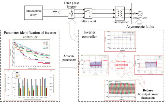
The asymmetric faults often cause the power grid current imbalance and power grid oscillation, which brings great instability risk to the power grid. To address this problem, this paper presented a modeling and parameter optimization method of grid-connected photovoltaic (PV) systems, considering the low voltage ride-through (LVRT) control. The harmonics of the grid current under asymmetric faults were analyzed based on the negative-sequence voltage feedforward control method. The notch filter was added to the voltage loop to filter out the harmonic components of the DC bus voltage and reduce the harmonic contents of the given grid current value. The proportional resonant (PR) controller was added to the current loop. The combination of these two components could reduce the 3rd, 5th, and 7th harmonics of the grid current and the output power fluctuation. Then, the parameters of the inverter controller were identified by the adaptive differential evolution (ADE) algorithm based on the sensitivity analysis. The effectiveness of the proposed method was compared with two other strategies under the asymmetric grid faults. The suppression of DC bus voltage fluctuation, power fluctuation, and low-order harmonics of the grid current all had better results, ensuring the safe and stable operation of the PV plant under grid faults.

1. Introduction

With the increasing demand for clean, safe, and efficient energy systems, the photovoltaic (PV) technology has attracted extensive attention [1,2,3,4,5]. In 2003, the requirements of low voltage ride-through (LVRT) for wind farms were added to the German grid code. Now the grid code has also been applied to the photovoltaic (PV) system [6]. The PV system should keep its connected mode once the fault occurs unless the fault causes the power system instability, and its inverter should make a rapid response to the fault. Therefore, the grid-connected PV inverters have been implanted higher requirements, especially those on the control under asymmetric faults.

Scholars have done a lot of research on the LVRT of PV generation systems. In [7], the conventional power closed-loop is adopted to maintain the power balance between front and rear stages for PV generation systems, which do not consider the asymmetric faults. However, the asymmetric faults appear more frequently than symmetrical faults in the actual grid operation. The grid current contains a large amplitude of negative-sequence components for asymmetric faults, which can lead to a high imbalance and harmonic increase of the grid current [8,9]. As a result, the inverter cannot operate stably. Therefore, the control strategies have been proposed to improve the LVRT capability of the inverter, such as the proportional-resonant (PR) control [10], the fuzzy logic control [11], and the coordinated control of PV energy storage system [12].

With the development of digital signal processing technology, complicated control strategies are applied to grid-connected inverters, such as the sliding mode control [13], the model predictive control [14], the neural network control [15], etc. To reduce the complexity of the control system, a robust control strategy without a phase-locked loop is used [16], which reduces the adjustment efforts of additional controller parameters. The negative-sequence feedforward control strategy in the d-q coordinate system has been proposed [17], but the negative-sequence voltage component is still not well suppressed. The existing researches mainly focus on the suppression methods of active power fluctuation [18], reactive power fluctuation [19], current harmonic [20], or combined targets [21,22]. However, there lack effective methods that can precisely analyze the harmonic components of various variables and suppress harmonics on the premise of power fluctuation suppression under asymmetric faults.

It is essential to obtain the parameters of the PV generation system [23]. Researchers have tried to use the heuristic algorithm that has no strict requirements for the objective function of identification [24,25,26]. The identification focuses on the parameters of PV arrays, controller, or limiters of PV inverter [27,28], but less for the LVRT control parameters. The LVRT control should be contained for the inverter that is the core of the grid-connected PV system, but its controller parameters are not easy to be obtained [29]. The identification based on measured data [30,31] is one of the feasible means to obtain parameters, which is an important link in standardized modeling. The appropriate disturbance signals should be chosen for parameter identification [29]. The single disturbance excitation method has been applied [32,33], but it lacks verification for various operating conditions.

Compared with previous studies, this paper is innovative in the following aspects:

(i)

The specific harmonic in the grid current and DC bus voltage was eliminated by the combination of the notch filter and PR controller based on the harmonic analysis, which is beneficial to improve the output power quality.

(ii)

The influence of inverter controller parameters on the transient process and the steady-state value was obtained through sensitivity analysis, which could guide the process of parameter identification.

(iii)

A disturbance setting suitable for parameter identification of the inverter controller considering LVRT capability was proposed.

(iv)

The optimal algorithm was selected through the parameter identification comparison of several heuristic algorithms, and the sensitivity analysis was verified. The strategy of identifying high-sensitivity parameters through ADE (i.e., adaptive differential evolution) algorithm could reliably obtain the controller parameters. The parameters of the actual PV power station were identified based on the measured data.

The organization of this paper is as follows. The harmonic analysis of the grid current is presented in Section 2. The inverter control model is built in Section 3. The influence of parameters perturbation of the inverter controller on the transient process and steady-state value of the system is obtained based on the sensitivity analysis in Section 4. Section 4 also proposes the optimal algorithm of PV inverter controller parameters. The results and discussion are presented in Section 5.

2. Analysis of Grid-connected PV System

2.1. PV Array Model

Figure 1 shows the equivalent model of the PV cell.

In Figure 1, U and I are the output voltage and current of PV cells, respectively. R_L is the load resistance. R_S and R_sh are the equivalent series resistance and parallel resistance of the PV cell, respectively. The I_d is the reverse saturation current of the diode. I_SC is the current source current.

The output characteristic of the PV cell is expressed as follows:

$$I=I_{sc}-I_{\mathrm{d}}(e^{\frac{q(U+I{R}_s)}{AkT}}-1)-\frac{U+I{R}_s}{R_{sh}}$$

(1)

where q is the electron charge with the value of 1.602 × 10⁻¹⁹ C, a is the constant of a PN junction curve (i.e., 1 ≤ a ≤ 2), and K is the Boltzmann constant with the value of 1.38 × 10⁻³² J/K.

Since Rsh is large, ignoring the (U + IR_s)/R_sh term in Equation (1) results in:

$$I=I_{sc}-C_1{I}_{sc}(e^{\frac{U}{C_2{U}_{oc}}}-1)$$

(2)

where $C_1=(1-\frac{I_{\mathrm{m}}}{I_{sc}})e^{-\frac{U_m}{C_2{U}_{oc}}}$ and $C_2=(\frac{U_m}{U_{oc}}-1)/\ln (1-\frac{I_{\mathrm{m}}}{I_{sc}})$ under standard working conditions.

Under general working conditions, the parameter expression is obtained by Equation (3).

$$\{\begin{array}{c}\mathsf{\Delta }T=T-T_{ref}\\ \mathsf{\Delta }G=\frac{G}{G_{ref}}-1\\ U_{oc}^{\prime }=U_{oc}(1-c\mathsf{\Delta }T)\ln (e+b\mathsf{\Delta }G)\\ I_{sc}^{\prime }=I_{sc}\frac{G}{G_{ref}}(1+a\mathsf{\Delta }T)\\ U_m^{\prime }=U_m(1-c\mathsf{\Delta }T)\ln (e+b\mathsf{\Delta }G)\\ I_m^{\prime }=I_m\frac{G}{G_{ref}}(1+a\mathsf{\Delta }T)\end{array}$$

(3)

In Equation (3), the typical values of correction factors, namely, a, b, and c are 0.0025, 0.5, and 0.00288, respectively. The PV array is composed of a series and parallel connection of the PV cell model.

2.2. Power Flow Analysis of the PV Inverter

According to Kirchhoff’s voltage and current laws, the mathematical model of the three-phase PV inverter in the two-phase synchronous rotating coordinate system under asymmetric grid faults is given by:

$$\{\begin{array}{l}{U}_d^{+}=e_d^{+}+L\frac{d{i}_d^{+}}{dt}+R{i}_d^{+}+\omega L{i}_q^{+}\\ U_d^{-}=e_d^{-}+L\frac{d{i}_d^{-}}{dt}+R{i}_d^{-}-\omega L{i}_q^{-}\\ U_q^{+}=e_q^{+}+L\frac{d{i}_q^{+}}{dt}+R{i}_q^{+}-\omega L{i}_d^{+}\\ U_q^{-}=e_q^{-}+L\frac{d{i}_q^{-}}{dt}+R{i}_q^{-}+\omega L{i}_d^{-}\end{array}$$

(4)

where ‘+’ and ‘−’ represent the positive and negative-sequence components of the grid voltage and grid current, respectively.

According to the mathematical model of grid-connected PV inverter and Equation (4), the equation for DC power balance without considering the loss of the PV inverter under asymmetric faults is expressed as:

$$C{U}_{dc}\frac{d{U}_{dc}}{dt}=P_{PV}-P$$

(5)

The instantaneous complex power output of PV inverter under asymmetric faults can be expressed as:

$$S_g=\frac{3}{2}{\dot{U}}_{\alpha \beta }{\dot{I}}_{\alpha \beta }=\frac{3}{2}(e^{j\omega }{\dot{U}}_{dq}^{+}+e^{-j\omega }{\dot{U}}_{dq}^{-})(e^{j\omega }{\dot{I}}_{dq}^{+}+e^{-j\omega }{\dot{I}}_{dq}^{-})$$

(6)

By combining Equations (5) and (6), the Equation (7) is obtained:

$$C{U}_{dc}\frac{d{U}_{dc}}{dt}=P_{PV}-[P_0+P_{c2}\cos (2\omega t)+P_{s2}\sin (2\omega t)]$$

(7)

As can be seen from Equation (7), when the asymmetrical fault occurs, the double fundamental frequency fluctuation of active power will cause the DC side capacitor of the inverter to be frequently charged and discharged. This causes the DC bus voltage fluctuation and affects the stability of the power system.

2.3. Harmonic Analysis of Grid Current

Based on the symmetrical component theory, the harmonic components of the grid current for asymmetry fault are analyzed in a synchronous rotating coordinate system. Figure 2 shows the spatial vector relationship of dq⁺ and dq⁻ in the αβ stationary coordinate system. The superscript "+" and "−" represent the positive and negative rotating coordinate systems, respectively. F represents the generalized voltage and current vectors.

In the case of asymmetric grid faults, the coordinate transformation relationship between the variables of the system can be expressed as:

$$\{\begin{array}{c}{F}_{dq}^{+}=F_{\alpha \beta }{e}^{-j\omega t}\\ F_{dq}^{-}=F_{\alpha \beta }{e}^{j\omega t}\\ F_{dq}^{+}=F_{dq}^{-}{e}^{-j2\omega t}\\ F_{dq}^{-}=F_{dq}^{+}{e}^{j2\omega t}\end{array}$$

(8)

$$\left[\begin{array}{c}{U}_{\mathrm{a}}\\ U_b\\ U_c\end{array}\right]=\sqrt{\frac{2}{3}}\left[\begin{array}{ccc}\cos \omega t& \cos (\omega t-{120}^{\circ })& \cos (\omega t+{120}^{\circ })\\ -\sin \omega t& -\sin (\omega t-{120}^{\circ })& -\sin (\omega t+{120}^{\circ })\\ \frac{1}{\sqrt{2}}& \frac{1}{\sqrt{2}}& \frac{1}{\sqrt{2}}\end{array}\right]\left[\begin{array}{c}{U}_d\\ U_q\\ U_0\end{array}\right]$$

(9)

According to Equation (8), the positive and negative sequence components of the variables in the positive and negative rotation coordinate system under asymmetric grid faults are shown as:

$$\{\begin{array}{c}{U}_{dq}=U_{dqp}^{+}+U_{dqn}^{-}=U_{dqp}^{+}+U_{dqn}^{+}{e}^{-j2\omega t}\\ I_{dq}=I_{dqp}^{+}+I_{dqn}^{-}=I_{dqp}^{+}+I_{dqn}^{+}{e}^{-j2\omega t}\end{array}$$

(10)

where the subscripts p and n represent positive and negative sequence components, respectively.

According to Equations (9) and (10), it can be known that under the asymmetric fault of the power grid, the grid voltage and grid current have the double fundamental frequency fluctuation in the positive and negative rotating coordinate system. The grid voltage has the triple fundamental frequency fluctuation, and the grid current also has the triple frequency fluctuation. Supposing only harmonic components that are integer multiples of the fundamental wave are considered, the grid voltage and grid current are shown in Equation (11).

$$\{\begin{array}{c}{U}_A={\displaystyle \sum _{\mathrm{k}=1}^{\infty }{U}_{km}\sin (k\omega t)}\\ U_B={\displaystyle \sum _{\mathrm{k}=1}^{\infty }{U}_{km}\sin \left[k(\omega t-\frac{2\pi }{3})\right]}\\ U_C={\displaystyle \sum _{\mathrm{k}=1}^{\infty }{U}_{km}\sin \left[k(\omega t+\frac{2\pi }{3})\right]}\end{array}\begin{array}{c}\end{array}\mathrm{and}\begin{array}{c}\end{array}\{\begin{array}{c}{I}_A={\displaystyle \sum _{\mathrm{k}=1}^{\infty }{I}_{km}\sin (k\omega t+{\mathsf{\Phi }}_k)}\\ I_B={\displaystyle \sum _{\mathrm{k}=1}^{\infty }{I}_{km}\sin \left[k(\omega t-\frac{2\pi }{3})+{\mathsf{\Phi }}_k\right]}\\ I_C={\displaystyle \sum _{\mathrm{k}=1}^{\infty }{I}_{km}\sin \left[k(\omega t+\frac{2\pi }{3})+{\mathsf{\Phi }}_k\right]}\end{array}$$

(11)

Assuming that the grid voltage and grid current have no harmonic components, it can be known from the analysis in Section 2.2 that the DC bus voltage contains the double fundamental frequency component. Ũ_dc is the ripple of the DC bus voltage shown in Equation (12).

$${\tilde{U}}_{dc}=\frac{P_{s2}}{2C\omega U_{dc}}\cos (2\omega t)-\frac{P_{c2}}{2C\omega U_{dc}}\sin (2\omega t)$$

(12)

For the inverter adopting dual-loop control, the d-axis reference value of the grid current is shown in Equation (13).

$$I_{dref}=(K_{PU}+\frac{K_{IU}}{s})(U_{dc}^{*}-{\overline{U}}_{dc}-{\tilde{U}}_{dc})=(K_{PU}+\frac{K_{IU}}{s})[U_{dc}^{*}-{\overline{U}}_{dc}-\frac{P_{s2}}{2C\omega U_{dc}}\cos (2\omega t)-\frac{P_{c2}}{2C\omega U_{dc}}\sin (2\omega t)]$$

(13)

According to Equation (13), there is the double fundamental frequency fluctuation in the d-axis reference value I_dref of the grid current. There is triple fundamental frequency fluctuation in the grid voltage and current after modulation, as U_3m ≠ 0 and I_3m ≠ 0. Without considering the fluctuation of the grid voltage and current caused by the negative sequence component, the double fundamental frequency component of I_dref also causes the ripple fundamental frequency fluctuation of the grid current. The mutual influence between harmonic voltage and harmonic current is ignored, and the decomposition of “U_AI_A” is taken as an example. According to Equation (11), the instantaneous active power can be expressed by Equation (14).

$$\begin{array}{l}P=U_A{I}_A+U_B{I}_B+U_C{I}_C\\ \begin{array}{l}\hfill \end{array}=\frac{1}{2}{U}_{k1}{I}_{k1}\cos ({\mathsf{\Phi }}_1)-\frac{1}{2}{U}_{k1}{I}_{k1}\cos (2\omega t+{\mathsf{\Phi }}_1)+U_{k1}{\displaystyle \sum _{k=2}^{\infty }{I}_{km}\sin (k\omega t+{\mathsf{\Phi }}_k)\sin (\omega t)}\\ \begin{array}{l}\hfill \end{array}+I_{k1}{\displaystyle \sum _{\mathrm{k}=1}^{\infty }{U}_{km}\sin (k\omega t)}\sin (\omega t+{\mathsf{\Phi }}_1)+U_B{I}_B+U_C{I}_C\end{array}$$

(14)

According to Equations (5) and (14), the DC bus voltage will appear in second and fourth harmonics because of the second and fourth harmonics in instantaneous active power. The reference value for the d-axis component of the grid current will appear in the 4th harmonic caused by the 3rd harmonic of the grid current. Therefore, the grid current will appear in the fifth harmonic. By analogy, the grid current has 3rd, 5th, 7th, and other low-order harmonics, and the DC bus voltage has 2nd, 4th, 6th, and other low-order harmonics.

3. Control Model for PV Inverter

The negative sequence voltage feedforward control method can suppress the negative sequence component under asymmetric faults, but there are still a large number of harmonics in the grid current and DC bus voltage, resulting in the fluctuation of several output variables [34,35] in the LVRT process. Therefore, it is necessary to filter out these harmonics, as well as to suppress the fluctuations of voltage, active, and reactive power simultaneously.

According to the analysis in Section 2.3, the grid current has odd harmonics, and the DC bus voltage has even harmonics under the conventional dual-loop control strategy when asymmetrical grid faults occur. The notch filter can eliminate the specific harmonics of the DC bus voltage. The PR controller is applied to eliminate the low-order harmonics of the grid current caused by the asymmetric faults. The outer-loop and inner-loop control model of the inverter is constructed by combining the notch filter and the PR controller. The improved model is used to achieve the purpose of DC bus voltage fluctuation and power fluctuation suppression.

3.1. Overall Control Model

Figure 3 shows the overall model of inverter control under grid faults. In Figure 3, The MPPT (i.e., maximum power point tracking) module is designed for the maximum power point tracking control. The DSOGI-PLL (i.e., double second order generalized integrator phase locked loop) module is designed to separate positive and negative sequence components and obtain the accurate phase. The SVPWM (i.e., space vector pulse width modulation) module is designed to generate drive signals.

The output U_g of the grid voltage amplitude calculation module is used to judge that the grid voltage is normal or not. The voltage loop outputs the active current reference value I_dref, and the reactive current reference value I_qref is zero during the normal operation.

The inverter control with reactive power priority is adopted in the case of grid voltage sags, which stops the MPPT control. When the new reference value is obtained through the active and reactive current reference value calculation module, the active power and reactive power input to the grid can be redistributed.

3.2. Grid Code for LVRT

The PV system should provide reactive power support under grid faults according to the requirements of the grid code [36]. The German grid codes are shown in Figure 4 and Figure 5.

The PV generation system tracks the voltage changes at the grid connection point during the fault, and it should output a certain amount of reactive current to maintain the voltage. At this time, the reference value of the reactive and active current can be calculated according to Equations (15) and (16).

$$i_{qref}^{*}=\{\begin{array}{l}{I}_q=0,\begin{array}{cc}\begin{array}{cc}\begin{array}{cc}\begin{array}{cc}& \end{array}& \end{array}& \end{array}& U_g\ge 0.9\begin{array}{l}\hfill \end{array}\mathrm{p}.\mathrm{u}.\end{array}\hfill \\ \begin{array}{l}{I}_q=\lambda (1-U_g)I_N,\begin{array}{cc}& (1-\frac{1}{\lambda })\begin{array}{l}\hfill \end{array}\mathrm{p}.\mathrm{u}.\le U_g\le 0.9\begin{array}{l}\hfill \end{array}\mathrm{p}.\mathrm{u}.\end{array}\hfill \\ I_q=I_N,\begin{array}{cc}\begin{array}{cc}\begin{array}{cc}\begin{array}{cc}& \end{array}& \end{array}& \end{array}& 0\le U_g\le (1-\frac{1}{\lambda })\begin{array}{l}\hfill \end{array}\mathrm{p}.\mathrm{u}.\end{array}\hfill \end{array}\hfill \end{array}$$

(15)

$$i_{dref}^{*}=\min (I_{dref},\sqrt{I_{\max }^2-i_{qref}^{*2}})$$

(16)

where λ ≥ 2, I_N is the rated current of the inverter, and I_max is the allowable maximum current.

3.3. Voltage Sag Fault Detection

Considering the voltage sag fault detection, the three-phase voltage can be expressed as:

$$U_{abc}=U_{abc}^f+U_{abc}^h=U_{abc}^{f\_s}-U_{abc}^{f\_c}+U_{abc}^h$$

(17)

where f represents the fundamental component, and h represents the harmonic component. s is the steady-state component, and c is the compensation component.

In this paper, the method of Kalman filter [37] for voltage sag detection can accurately detect the voltage sag amplitude under the influence of harmonics, which has strong robustness.

The amplitude of the fundamental wave of grid voltage is calculated as follows:

$$U_{\mathrm{g}}=\sqrt{{\frac{{(X_{\alpha }^f)}^2+(X_{\beta }^f)}{2}}^2}$$

(18)

where X is the estimated value of the Kalman filter.

The voltage drop detection model is formed together with the positive and negative sequence separation module [38] and a positioning module [39]. The position module includes a mathematical morphology filter (MMF) and a grille fractal (GF). Figure 6 shows the voltage sag detection model. Figure 7 shows the fundamental signal detected under a voltage sag of 50%.

3.4. Outer-Loop and Inner-Loop Controls of the PV Inverter

Figure 8 shows the outer-loop and inner-loop control block diagrams of the inverter controller.

The outer-loop control eliminates the 2nd, 4th, 6th harmonic components by adding a notch filter to the DC bus voltage feedback U_dc under grid faults. It further reduces the fluctuation of DC bus voltage by feeding the instantaneous current forward at the DC side. The reference value of the active output current is shown in Equation (19).

$$\begin{array}{l}{I}_{dref}=\{\begin{array}{cc}(K_{PU}+\frac{K_{IU}}{s})(U_{dc}^{*}-U_{dc}·G_{(\mathrm{s})}^{\prime })+\frac{P^{*}}{U_{dc}}& U_g<T{h}_2\\ (K_{PU}+\frac{K_{IU}}{s})(U_{dc}^{*}-U_{dc}·G_{(\mathrm{s})}^{\prime })& U_g\ge T{h}_2\end{array}\begin{array}{cc}& \end{array}\\ \mathrm{where}\begin{array}{c}\end{array}{G}_{(S)}^{\prime }=(\frac{s^2+{\omega }_2^2}{s^2+K{\omega }_2^{2}s+{\omega }_2^2})(\frac{s^2+{\omega }_4^2}{s^2+K{\omega }_4^{2}s+{\omega }_4^2})(\frac{s^2+{\omega }_6^2}{s^2+K{\omega }_6^{2}s+{\omega }_6^2})\end{array}$$

(19)

where P^*/U_dc is the feed-forward values of instantaneous current at the DC side, and Th₂ is 0.9. K = 1/Q, and Q is the quality factor.

The influence of the parameter error of notch filter on the overall system is analyzed in Figure 9. The sensitivity analysis method is used. The parameter perturbation is 5%, the disturbance is set at 0.1 s, and the grid voltage drops to 0.4 per unit (pu). The sensitivities of the parameter error to active power, reactive power, DC bus voltage, and voltage and current in AC side are obtained as follows:

The average trajectories sensitivity of P with a unit of kW, Q with a unit of kVar, U_dc with a unit of V, U_A with a unit of V, and I_A with a unit of A is 0.192, 0.110, 0.002, 0.002, and 1.550, respectively. It can be seen from the trajectory sensitivity analysis that parameter error of K has an obvious influence on P, Q, U_dc, and entire influence on AC voltage and current. The AC current has the most effect on the current ripple. Therefore, a proper setting of K is conducive to the stable operation of the PV system.

The inner-loop suppresses the negative sequence component of the grid voltage by controlling the negative sequence component of the voltage to zero when the grid voltage is unbalanced. However, there are low-order harmonics in the grid current under this control strategy, and the low-order harmonics, such as 3rd, 5th, and 7th, are significant. In this paper, the PR controller is used for harmonic suppression.

Compared with the proportional-integral (PI) controller, the gain of the inner-loop PR controller is much larger, and it is easier to extract the signal characteristics of the resonant frequency, so as to realize the control without steady-state error. The PR controller cannot only ensure the good power quality of the grid current but also help to decrease the power fluctuation. Its transfer function is shown in Equation (20).

$$G_{PR}(s)=K_{PI}+\frac{2K_{RI}s}{s^2+{\omega }_0^2}+{\displaystyle \sum _{h=2,4,6}\frac{K_{Rh}s}{s^2+{(h{\omega }_0)}^2}}$$

(20)

In the engineering process, a low-pass filter is usually used to replace the pure integration link in the PR controller to improve the anti-interference performance and system stability. Figure 10 shows the amplitude-frequency and phase-frequency characteristic curves of the transfer function of the quasi-PR controller. Its transfer function, with harmonic suppression control, and simplified function are expressed as:

$$\begin{array}{l}{G}_{PR}^{\prime }(s)=K_{PI}+\frac{2{\omega }_c(s+{\omega }_c)}{s^2+2{\omega }_{c}s+{\omega }_c^2+{\omega }_0^2}{K}_{RI}+{\displaystyle \sum _{h=2,4,6}\frac{2K_{Rh}{\omega }_{ch}(s+{\omega }_{ch})}{s^2+2{\omega }_{ch}s+{\omega }_{ch}^2+{(h{\omega }_0)}^2}}\\ G_{PR}^{\prime }(s)=K_{PI}+\frac{2{\omega }_{c}s}{s^2+2{\omega }_{c}s+{\omega }_0^2}{K}_{RI}+{\displaystyle \sum _{h=2,4,6}\frac{2K_{Rh}{\omega }_{ch}s}{s^2+2{\omega }_{ch}s+{(h{\omega }_0)}^2}}\mathrm{while}{\omega }_{\mathrm{c}},{\omega }_{\mathrm{ch}}\ll {\omega }_0\end{array}$$

(21)

By using the PR controller and negative sequence voltage feedforward control, the inner-loop mathematical model can be expressed as:

$$\{\begin{array}{c}{U}_d=u_d^{+}+G_{PR}^{\prime }(s)(i_{dref}^{*}-i_d)-\omega L_2{i}_q-u_d^{-}\\ U_q=u_q^{+}+G_{PR}^{\prime }(s)(i_{qref}^{*}-i_q)-\omega L_1{i}_d-u_q^{-}\end{array}$$

(22)

From Equation (22) and Figure 8, the negative sequence component of feed-forward grid voltage is offset with the negative sequence component of inverter output voltage under asymmetric faults for the inner-loop control.

4. Parameter Identification

4.1. Parameter Identification Process

Both the outer-loop parameters (i.e., K_PU and K_IU) and the inner-loop parameters (i.e., K_PI and K_RI) have a great influence on the output power. They are selected for identification. The ADE, GA (i.e., genetic algorithm), FPA (i.e., flower pollination algorithm), PSO (i.e., particle swarm optimization), CPSO (i.e., chaos particle swarm optimization) [40], BBO (i.e., biogeography-based optimization), and ALO (i.e., ant lion optimization) algorithms are selected to identify the parameters in the established PV generation system model. The ADE algorithm has strong global and local search abilities. The adaptive mutation operator was introduced to avoid premature convergence as follows:

$$F=F_0\times 2^{\tau },\tau =e^{1-\frac{G_m}{G_m+1-G}}$$

(23)

where F is the scaling factor, and F₀ is the mutation rate. In this paper, F₀ = 0.5.

Figure 11 shows the schematic of controller parameter identification.

The fitness function J is defined as:

$$J=\frac{1}{n}\{{\displaystyle \sum _{k=1}^n[U_d(k)-U_d^{\prime }}(k){]}^2+{\displaystyle \sum _{k=1}^n[}{U}_q(k)-U_q^{\prime }(k){]}^2\}$$

(24)

4.2. Sensitivity Analysis on Controller Parameters

The sensitivity analysis [41] is performed on the parameters of the inverter controller to obtain the parameter identifiability. The trajectory sensitivity is expressed as:

$${\tilde{G}}_{\mathrm{k}}=\underset{\mathsf{\Delta }{a}_j\to 0}{\lim }\frac{\left[{\mathrm{y}}_i(a_1,\dots a_j+\mathsf{\Delta }{a}_j,\dots a_m,t)-{\mathrm{y}}_i(a_1,\dots a_j-\mathsf{\Delta }{a}_j,\dots a_m,t)\right]/y_{i0}}{2\mathsf{\Delta }{a}_j/a_{j0}}$$

(25)

In order to compare the trajectory sensitivity of each parameter, the average value of the absolute value of sensitivity is calculated as the sensitivity index, that is:

$$H_{\mathrm{ij}}=\frac{1}{k}{\displaystyle \sum _{k=1}^K\left|\widetilde{G_{\mathrm{k}}}\right|}$$

(26)

where k is the total number of points for trajectory sensitivity.

The setting of the inner-loop and outer-loop parameters of the inverter controller has an important influence on the dynamic and static characteristics of the system. The initial value of the output is 1 per unit (pu). When the disturbance occurs at 0.1 s, the voltage sag of phase A is 60%, and it lasts for 0.1 s. The simulation is carried out under the condition that the inner-loop and outer-loop parameters are perturbed by 1% and 5%, respectively. The trajectory sensitivity analysis takes the I_d as an example, and the sensitivity curves are recorded in Figure 12, and the results of the sensitivity analysis are recorded in

Table 1. The result of the sensitivity analysis of parameter.

Parameter	Sensitivity Index		Terminal Value Id
	Disturbances of ±1%	Disturbances of ±5%	Disturbances of ±1%	Disturbances of ±5%
KPI	0.011495	0.011654	1.067324/1.067162	1.067279/1.066989
KRI	0.009406	0.009517	1.067011/1.066916	1.066982/1.067131
KPU	0.002546	0.002653	1.067043/1.067015	1.067836/1.068014
KIU	0.000545	0.000604	1.067157/1.066861	1.066882/1.066643
Parameter	Terminal Value Iq		Terminal Value Udc
	Disturbances of ±1%	Disturbances of ±5%	Disturbances of ±1%	Disturbances of ±1%
KPI	1.034561/1.030714	1.040867/1.029032	1.003369/1.003442	1.003229/1.003156
KRI	1.029934/1.025226	1.032258/1.036151	1.003422/1.003455	1.003445/1.003313
KPU	1.036331/1.034835	1.033091/1.034272	1.003295/1.003437	1.002558/1.003027
KIU	1.032258/1.036151	1.035354/1.037577	1.003229/1.003156	1.003319/1.003560
Parameter	Terminal Value P		Terminal Value Q
	Disturbances of ±1%	Disturbances of ±5%	Disturbances of ±1%	Disturbances of ±5%
KPI	0.994143/0.994477	0.994720/0.994523	1.030622/1.025733	1.038964/1.024035
KRI	0.994261/0.993694	0.994068/0.994033	1.024949/1.020192	1.027286/1.031219
KPU	0.994582/0.994320	0.995425/0.994757	1.031489/1.029887	1.028135/1.029323
KIU	0.994720/0.994523	0.994198/0.993845	1.027286/1.031219	1.030419/1.032668

.

It can be seen from Figure 12 and Table 1 that after the occurrence of voltage sag, the sensitivity fluctuation amplitude of the inner-loop parameters is larger than that of outer-loop parameters. The trajectory sensitivity value for the perturbation of K_PI is the largest of the four parameters, so adjusting the inner-loop proportion coefficient has the greatest influence on the system.

It can also be seen from Table 1 that under the perturbation of both 1% and 5%, the sensitivity index of K_PI is the highest among the four parameters, indicating that it has the greatest impact on the system transient process. The sensitivity index follows K_PI > K_RI > K_PU > K_IU. The parameter perturbation influence on the terminal value of I_q and Q is greater than that of I_d and P. Under the perturbation of K_PI, the variable terminal values deviate largest, and the influence of the perturbation of K_RI is less. The parameters of K_PU and K_IU have less influence on the variable terminal values.

In summary, the impact of K_PI has a larger effect under deeper parameter disturbance. The trajectory sensitivity of K_IU is the lowest, so it is not easy to identify. Therefore, K_IU is calculated by the analytical method to improve identification efficiency.

4.3. Parameter Identification Results

In the MATLAB 2018a (MathWorks, Natick, MA, USA) environment, the different algorithms are used to identify the controller parameters of the grid-connected inverter. The algorithms are identified for many times, and the identification results are shown in Figure 13 and Figure 14.

It can be seen from Figure 13 and Figure 14 that the initial convergence rate of ADE and FPA algorithm is better, but the final identification accuracy of the FPA algorithm is poor. In general, the FPA, PSO, CPSO, ALO, and BBO algorithms have lower identification accuracy compared with GA and ADE algorithms. Although GA and ADE algorithms have similar identification accuracy, the parameter identification results differ obviously. This is because there are suboptimal values for outer-loop parameters. For identification time, T_FPA > T_ADE > T_CPSO > T_GA > T_PSO > T_ALO > T_BBO. If the requirement of identification accuracy is not high, the ALO and BBO algorithms can be used as fast identification methods. The ADE algorithm has better initial convergence speed and identification accuracy, which is selected for parameter identification. In addition, the identification effect of the above algorithms is the worst for K_IU and best for K_PI, which proves the results of the sensitivity analysis. Therefore, K_IU can be calculated by the analytical method.

The model runs under steady-state conditions, and the PV modules operate under standard test conditions (i.e., S = 1000 W/m², T = 25 °C). The disturbances are set as:

(a)

It is assumed that the voltage sag occurs in phase A at 0.1 s, and the grid voltage drops to 0.4 pu. The fault is removed at 0.3 s.

(b)

It is assumed that the voltages drop to 0.4 pu in phase B and phase C at 0.1 s, and then the fault is removed at 0.3 s.

(c)

It is assumed that when the system runs stably to 0.1 s, a three-phase voltage drop occurs, and the grid voltage drops to 0.4 pu. The fault is removed at 0.3 s.

The controller parameter values of a grid-connected inverter are determined by the system amplitude margin, phase margin, and cut-off frequency [42]. In the process of iteration, it should be judged whether the individual satisfies the boundary conditions of the solution space to ensure the validity of the solution; otherwise, the individual is regenerated by a random method. The boundary conditions and reference values are set in

Table 2. Solution space boundary condition and reference value.

Parameter	XMIN	XMAX	Reference Value
KPU	0	100	6.7
KPI	0	10	0.9
KRI	0	150	10

.

According to the sensitivity analysis and multi-algorithm identification results, the ADE algorithm is used to identify the inner-loop parameters (K_PI, K_RI) and outer-loop parameter (K_PU).

Table 3. Parameter identification results under ADE algorithm.

Parameter		Single-Phase	Two-Phase	Three-Phase
KPU	Identification	6.6959	6.6941	6.6659
	Error rate/%	0.0612	0.0881	0.5089
KPI	Identification	0.9000	0.9002	0.8998
	Error rate/%	0.0000	0.0222	0.0222
KRI	Identification	10.0000	10.0009	10.0919
	Error rate/%	0.0000	0.0090	0.9190
Fitness value		2.7 × 10−13	2.5 × 10−12	1.2 × 10−11

shows the parameter identification results.

According to Table 3, the identification results are good under each working condition. The other three parameters can be identified more accurately if the K_IU parameter is obtained firstly. It can also be seen from the fitness values in Table 3 that the identification accuracy is higher in the case of single-phase voltage sag.

Figure 15 shows the simulation and tested curves of the model under phase A voltage sag. The results show that the simulation curves are consistent with the tested curves, and the simulation errors are small, which verifies the validity and rationality of the established model and its parameter selection. Good results have been achieved under the other working conditions, and the model parameters can be obtained effectively.

4.4. Measurement Identification of the PV Plant

To further verify the adaptability of the model and parameters, the disturbance tests of the inverter are performed on PV power stations, including active and reactive power step disturbances.

Table 4. Simulation parameters of the actual PV generation system.

Parameter	Meaning of Parameter	Value
Prated	Rated power	0.5 MW
Udc	DC bus voltage	900 V
UPV	PV cell voltage	85.3 V
IPV	PV cell current	6.09 A
C	DC side capacitance	14.4 mF
L1	Filter inductance	240 mH
L2	Filter inductance	60 mH
f	Switching frequency	1.228 kHz

shows the parameter settings of the established model for the actual PV generation system.

According to the light conditions during the test, the active output power of the inverter is limited to 517 kW. The active power setting value of the inverter is changed about ±10% of the rated power, and then the voltage, current, and power changes of the inverter’s AC side are recorded. Figure 16 shows the dynamic output curves under the same conditions compared with measured data.

It can be seen from Figure 16 that when the active power step disturbance occurs, the phase voltage U_ab remains stable, while the phase A current and active power decrease with the disturbance. The parameters are identified with the measured data in other test conditions, and the results are consistent with the measured data, which proves the accuracy and effectiveness of the model under the disturbance.

5. Results and Discussion

To further verify the applicability of proposed control and parameter optimization, a simulation model of a 250 kW grid-connected PV generation system is built upon the Matlab/Simulink (version 2018a, MathWorks, Natick, MA, USA) simulation platform. The parameters of the established model are listed in

Table 5. Simulation parameters.

Parameter	Meaning of Parameter	Value
Prated	Rated power	0.25 MW
Udc	DC bus voltage	580 V
Um	Voltage at maximum power	72.6 V
Im	Current at maximum power	5.69 A
Uoc	Open circuit voltage	85.3 V
Isc	Short-circuit current	6.09 A
m	Serial number	7
n	Parallel number	88
C	DC side capacitance	1500 µF
LF	Inductor of the boost converter	10 mH
L	Filter inductor	0.5 mH
f	Switching frequency	1.228 kHz
KPU	Proportional coefficient of voltage loop	6.7
KIU	Integral coefficient of voltage loop	44.5
KPI	Proportional coefficient of current loop	0.9
KRI	Resonant coefficient of current loop	10
KRh	Resonant coefficient in harmonics suppression control	22
ωc	Cut-off frequency at fundamental frequency	π rad/s
ωch	Cut-off frequency at h times fundamental frequency	π × h rad/s

.

(a)

It is assumed that when the system operates steadily at 0.1 s, the voltage sag occurs in phase A, and the grid voltage drops to 0.4 pu (i.e., condition One). The fault is removed at 0.3 s.

(b)

Different from condition One, the voltages drop to 0.4 pu in phase B and phase C at 0.1 s, and the fault is removed at 0.3 s for condition Two.

Figure 17 and Figure 18 show the operating characteristics of three control modes under each working condition. The control modes are shown in

Table 6. The control modes for simulation operation.

Control Modes	Descriptions
Strategy One	The traditional voltage and current dual-loop control strategy is adopted, and the PI (proportional-integral) controller is used for both outer and inner loops. This strategy does not contain asymmetric fault control.
Strategy Two	The negative sequence voltage feedforward control is adopted in the inner-loop, and a notch filter is added to the DC bus voltage feedback to eliminate harmonics in the outer-loop. The PI controller is used for both outer and inner loops.
Strategy Three	The PR (proportional-resonant) controller with harmonic suppression is adopted in the inner-loop, and the other control strategies are the same as strategy Two.

.

It can be seen that under two different working conditions, the grid voltage imbalance is more severe in Figure 18. From Figure 17a and Figure 18a, the DC bus voltage increases rapidly at the moment of the grid fault under the traditional PI control strategy (i.e., strategy One), destroying the safe and stable operation. It responds to the fault immediately under strategy Three, and the overall fluctuation of DC bus voltage is small.

From Figure 17b,c, the active and reactive power of strategy One fluctuate dramatically when the grid voltage is unbalanced. The negative sequence voltage feedforward control based on the notch filter and the PI controller (i.e., strategy Two) reduces the power fluctuation, but the output power waveform still fluctuates more significantly compared with that of strategy Three. The power fluctuations are relatively stable by using the improved negative sequence voltage feedforward control based on the notch filter and the PR controller (i.e., strategy Three). Figure 18b,c show that the power fluctuations are more significant due to the increase of the imbalance degree. From Figure 17d and Figure 18d, the output current is effectively limited within 1.1 pu, which avoids overcurrent impulse.

From Figure 17e and Figure 18e, the total harmonic distortion (THD) of the grid current is larger under strategy One, and the harmonics contents, such as 3rd, 5th, and 7th, are high. The third harmonic is 13.6% and 16%, respectively, under two working conditions. Figure 17f,g and Figure 18f,g show that the 3rd, 5th, and 7th harmonic components of grid current under strategy Three are significantly reduced, and the current THD is controlled within 5%. The entire system with strategy Three improves the power quality in the case of grid voltage sags, which also has a smooth transition before, during, and after the faults, improving the dynamic control performance.

Figure 19 shows the operating characteristics of the proposed model under strategy Three, while the power grid suffers symmetrical faults. The three-phase voltage drops to 0.4 pu at 0.1 s, and the fault is removed at 0.3 s. The results show that the grid current amplitudes and THD values are restricted within safe limits. Due to the reactive power support during voltage sag, the grid-connected PV system can operate safely and stably. Therefore, the established model can also satisfy the LVRT requirements under the symmetric grid fault.

Figure 20 shows the influence of parameter identification on the control effect. Based on the identification results, a −5% error is set for K_PI, K_RI, K_PU, K_IU, respectively. Here, the simulation results of ±5% error under different working conditions are similar, so the experimental results under −5% error in case of phase A voltage sag are analyzed. It can be seen from Figure 20 that the errors of K_PI, K_RI, K_PU have a great influence on the output curve of the PV system, and the error of K_IU has little influence. The DC bus voltage, active power, and reactive power will fluctuate, and the AC side over-current will occur in the LVRT process if K_PI, K_RI, or K_PU cannot be identified accurately. According to the obtained identification results, the PV system can operate stably under strategy Three.

6. Conclusions

This paper proposed an improved method of modeling and parameter optimization without complicated control. According to the trajectory sensitivity analysis and multi-parameter identification performance comparison, the strategy of identifying high-sensitivity parameters through the ADE algorithm could reliably obtain the controller parameters based on the measured data. The response of the proposed method was compared with the PI control strategy, and the effect of the PR controller on power fluctuation suppression was demonstrated. The proposed model ensured the stability of the DC bus voltage and the output power of the PV generation system under asymmetric grid faults and effectively suppressed the harmonics of the grid current. It was conducive to the smooth transition of the power grid during the period of LVRT.

The simulation results verified the feasibility of the grid-connected PV generation system under asymmetric and symmetric faults. The proposed model and parameter identification method lay a foundation for building a high-reliability transient equivalent model of the PV generation system during grid faults.

References

- Ludin, N.; Mustafa, N.; Hanafiah, M.; Ibrahim, M.A.; Teridi, M.A.M.; Sepeai, S.; Zaharim, A.; Sopian, K. Prospects of life cycle assessment of renewable energy from solar photovoltaic technologies: A review. Renew. Sustain. Energy Rev. 2018, 96, 11–28. [Google Scholar] [CrossRef]
- Annapoorna, C.; Saha, K.; Mithulananthan, N. Harmonic impact of high penetration photovoltaic system on unbalanced distribution networks–learning from an urban photovoltaic network. IET Renew. Power Gener. 2016, 10, 485–494. [Google Scholar]
- Oon, K.; Tan, C.; Bakar, A.; Che, H.; Mokhlis, H.; Illias, H. Establishment of fault current characteristics for solar photovoltaic generator considering low voltage ride through and reactive current injection requirement. Renew. Sustain. Energy Rev. 2018, 92, 478–488. [Google Scholar] [CrossRef]
- Zhu, Y.; Kim, M.K.; Wen, H. Simulation and analysis of perturbation and observation-based self-adaptable step size maximum power point tracking strategy with low power loss for photovoltaics. Energies 2019, 12, 92. [Google Scholar] [CrossRef] [Green Version]
- Benali, A.; Khiat, M.; Allaoui, T.; Denaï, M. Power quality improvement and low voltage ride through capability in hybrid wind-PV farms grid-connected using dynamic voltage restorer. IEEE Access 2018, 6, 68634–68648. [Google Scholar] [CrossRef]
- BDEW. Technical Guideline, Generating Plants Connected to the Medium-Voltage Network; BDEW: Berlin, Germany, 2008. [Google Scholar]
- Yang, F.; Yang, L.; Ma, X. An advanced control strategy of PV generation system for low-voltage ride-through capability enhancement. Sol. Energy 2014, 109, 24–35. [Google Scholar] [CrossRef]
- Nasiri, M.; Mohammadi, R. Peak current limitation for grid side inverter by limited active power in PMSG-based wind turbines during different grid faults. IEEE Trans. Sustain. Energy 2017, 8, 3–12. [Google Scholar] [CrossRef]
- Camacho, A.; Castilla, M.; Miret, J.; Borrell, A.; De Vicuña, L.G. Active and reactive power strategies with peak current limitation for distributed generation inverters during unbalanced grid faults. IEEE Trans. Ind. Electron. 2015, 62, 1515–1525. [Google Scholar] [CrossRef] [Green Version]
- Xu, L.; Han, M. Control strategy of low-voltage ride-through for micro-grid under asymmetric grid voltage. High Power Convert. Technol. 2016, 3, 36–39. [Google Scholar]
- Yassin, H.; Hanafy, H.; Hallouda, M. Enhancement low-voltage ride through capability of permanent magnet synchronous generator-based wind turbines using interval type-2 fuzzy control. IET Renew. Power Gener. 2016, 10, 339–348. [Google Scholar] [CrossRef]
- Mahmud, N.; Zahedi, A.; Mahmud, A. A cooperative operation of novel PV inverter control scheme and storage energy management system based on ANFIS for voltage regulation of grid-tied PV generation system. IEEE Trans. Ind. Inf. 2017, 13, 2657–2668. [Google Scholar] [CrossRef]
- Merabet, A.; Labib, L.; Ghias, A.; Ghenai, C.; Salameh, T. Robust feedback linearizing control with sliding mode compensation for a grid-connected photovoltaic inverter system under unbalanced grid voltages. IEEE J. Photovolt. 2017, 7, 828–838. [Google Scholar] [CrossRef]
- Moghadasi, A.; Sargolzaei, A.; Anzalchi, A.; Moghaddami, M.; Khalilnejad, A.; Sarwat, A. A model predictive power control approach for a three-phase single-stage grid-tied PV module-integrated converter. IEEE Trans. Ind. Appl. 2018, 54, 1823–1831. [Google Scholar] [CrossRef]
- Lin, F.; Lu, K.; Ke, T. Probabilistic wavelet fuzzy neural network based reactive power control for grid-connected three-phase PV generation system during grid faults. Renew. Energy 2016, 92, 437–449. [Google Scholar] [CrossRef]
- Adeel, S.; Salim, I. A robust control scheme for grid-connected photovoltaic converters with low-voltage ride-through ability without phase-locked loop. ISA Trans. 2019, 96, 289–298. [Google Scholar]
- Vincenti, D.; Jin, H. A three-phase regulated PWM rectifier with on-line feedforward input unbalance correction. IEEE Trans. Ind. Electron. 1994, 41, 526–532. [Google Scholar] [CrossRef]
- Sosa, J.; Castilla, M.; Miret, J.; Matas, J.; Al-Turki, Y. Control strategy to maximize the power capability of PV three-phase inverters during voltage sags. IEEE Trans. Power Electron. 2016, 31, 3314–3323. [Google Scholar] [CrossRef] [Green Version]
- Sufyan, M.; Rahim, N.; Eid, B.; Raihan, S. A comprehensive review of reactive power control strategies for three phase grid connected photovoltaic systems with low voltage ride through capability. J. Renew. Sustain. Energy 2019, 11, 042701. [Google Scholar] [CrossRef]
- Zhou, N.; Ye, L.; Lou, X.; Wang, Q. Novel optimal control strategy for power fluctuation and current harmonic suppression of a three-phase photovoltaic inverter under unbalanced grid faults. Int. Trans. Electr. Energy Syst. 2015, 26, 1049–1065. [Google Scholar] [CrossRef]
- Al-Shetwi, A.; Sujod, M.; Blaabjerg, F. Low voltage ride-through capability control for single-stage inverter-based grid-connected photovoltaic power plant. Sol. Energy 2018, 159, 665–681. [Google Scholar] [CrossRef] [Green Version]
- Brandao, D.; Mendes, F.; Ferreira, R.; Silvaand, S.; Pires, I. Active and reactive power injection strategies for three-phase four-wire inverters during symmetrical/asymmetrical voltage sags. IEEE Trans. Ind. Appl. 2019, 55, 2347–2355. [Google Scholar] [CrossRef]
- Chen, X.; Kun, Y.; Wen, D.; Wen, Z.; Guo, L. Parameters identification of solar cell models using generalized oppositional teaching learning based optimization. Energy 2016, 99, 170–180. [Google Scholar] [CrossRef]
- Li, S.; Gu, Q.; Gong, W.; Ning, B. An enhanced adaptive differential evolution algorithm for parameter extraction of photovoltaic models. Energy Convers. Manag. 2020, 205, 112443. [Google Scholar] [CrossRef]
- Ebrahimi, S.; Salahshour, E.; Malekzadeh, M.; Gordillo, F. Parameters identification of PV solar cells and modules using flexible particle swarm optimization algorithm. Energy 2019, 179, 358–372. [Google Scholar] [CrossRef]
- Valdivia-González, A.; Zaldívar, D.; Cuevas, E.; Pérez-Cisneros, M.; Fausto, F.; González, A. A chaos-embedded gravitational search algorithm for the identification of electrical parameters of photovoltaic cells. Energies 2017, 10, 1052. [Google Scholar] [CrossRef] [Green Version]
- Zhang, J.; Sun, Y.; Liu, M.; Dong, W.; Han, P. Research on modeling of microgrid based on data testing and parameter identification. Energies 2018, 11, 2525. [Google Scholar] [CrossRef] [Green Version]
- Yu, K.; Qu, B.; Yue, C.; Ge, S.; Chen, X.; Liang, J. A performance-guided JAYA algorithm for parameters identification of photovoltaic cell and module. Appl. Energy 2019, 237, 241–257. [Google Scholar] [CrossRef]
- Liu, Z.; Wu, H.; Jin, W.; Xu, B.; Ji, Y.; Wu, M. Two-step method for identifying photovoltaic grid-connected inverter controller parameters based on the adaptive differential evolution algorithm. IET Gener. Trans. Distrib. 2017, 11, 4282–4290. [Google Scholar] [CrossRef]
- Mahmoud, Y.; El-Saadany, E. A photovoltaic model with reduced computational time. IEEE Trans. Power Electron. 2015, 62, 3534–3544. [Google Scholar] [CrossRef]
- Yu, K.; Liang, J.; Qu, B.; Cheng, Z.; Wang, H. Multiple learning backtracking search algorithm for estimating parameters of photovoltaic models. Appl. Energy 2018, 226, 408–422. [Google Scholar] [CrossRef]
- Ma, J.; Bi, Z.; Ting, T.; Hao, S.; Hao, W. Comparative performance on photovoltaic model parameter identification via bio-inspired algorithms. Sol. Energy 2016, 132, 606–616. [Google Scholar] [CrossRef]
- Chen, Z.; Yuan, X.; Tian, H.; Ji, B. Improved gravitational search algorithm for parameter identification of water turbine regulation system. Energy Convers. Manag. 2014, 78, 306–315. [Google Scholar] [CrossRef]
- Kamil, H.S.; Said, D.M.; Mustafa, M.W.; Miveh, M.R.; Ahmad, N. Low-voltage ride-through methods for grid-connected photovoltaic systems in microgrids. Int. J. Power Electron. Drive Syst. 2018, 9, 1834–1841. [Google Scholar]
- Gelma, B.; Li, W.; Chao, P.; Peng, S. A comprehensive LVRT strategy of two-stage photovoltaic systems under balanced and unbalanced faults. Int. J. Electr. Power Energy Syst. 2018, 103, 288–301. [Google Scholar]
- Yang, Y.; Wang, H.; Blaabjerg, F. Reactive power injection strategies for single-phase photovoltaic systems considering grid requirements. IEEE Trans. Ind. Appl. 2014, 50, 4065–4076. [Google Scholar] [CrossRef] [Green Version]
- Xue, S.; Cai, J. An advanced detection method for three-phase voltage sag. Proc. CSEE 2012, 32, 92–97. [Google Scholar]
- Ke, C.; Wu, A.; Bing, C.; Yi, L. Measuring and reconstruction algorithm based on improved second-order generalised integrator configured as a quadrature signal generator and phase locked loop for the three-phase AC signals of independent power generation systems. IET Power Electron. 2016, 9, 2155–2161. [Google Scholar] [CrossRef]
- Li, G.; Luo, Y.; Zhou, M.; Wang, Y. Power quality disturbance detection and location based on mathematical morphology and grille fractal. Proc. CSEE 2006, 26, 25–30. [Google Scholar]
- Wang, L.; Qiao, T.; Zhao, B.; Zeng, X. Modeling and parameter identification of grid-connected PV system during asymmetrical grid faults. In Proceedings of the IEEE 3rd Conference on Energy Internet and Energy System Integration, Changsha, China, 8–10 November 2019; pp. 2086–2090. [Google Scholar]
- Wang, L.; Zhao, J.; Liu, D.; Lin, Y.; Zhao, Y.; Lin, Z.; Zhao, T.; Lei, Y. Parameter identification with the random perturbation particle swarm optimization method and sensitivity analysis of an advanced pressurized water reactor nuclear power plant model for power systems. Energies 2017, 10, 173. [Google Scholar] [CrossRef] [Green Version]
- Liu, F.; Zhou, Y.; Duan, S.; Yin, J.; Liu, B.; Liu, F. Parameter Design of a Two-current-loop controller used in a grid-connected inverter system with LCL filter. IEEE Trans. Power Electron. 2009, 56, 4483–4491. [Google Scholar]
Figure 1.
Equivalent model of the photovoltaic (PV) cell.
Figure 2.
Vector diagram of the positive and negative synchronous rotation coordinates.
Figure 3.
Model of the inverter control.
Figure 4.
LVRT (low voltage ride-through) curves in German grid code.
Figure 5.
Reactive power configuration during LVRT.
Figure 6.
Principle diagram of voltage sag fault detection.
Figure 7.
Detected value of fundamental signal: (a) Voltage sag initiation process; (b) Voltage sag recovery process.
Figure 8.
Control block diagrams of the inverter controller: (a) Outer-loop control block diagram; (b) Inner-loop control block diagram.
Figure 9.
Trajectories sensitivity of notch filter parameters: (a) Active power sensitivity; (b) Reactive power sensitivity; (c) DC bus voltage sensitivity; (d) Phase A voltage sensitivity; (e) Phase A current sensitivity;
Figure 10.
Amplitude and frequency characteristic curves of the quasi-PR (proportional resonant) controller model.
Figure 11.
Schematic diagram of controller parameter identification.
Figure 12.
Dynamic response to perturbation of controller parameters: (a) Inner-loop parameters KPI; (b) Inner-loop parameters KRI; (c) Outer-loop parameters KPU; (d) Outer-loop parameters KIU.
Figure 13.
Convergence curves of different heuristic algorithms.
Figure 14.
Parameters identification results of different heuristic algorithms.
Figure 15.
Comparison between simulation and tested curves under phase A voltage sag: (a) Simulation and tested curves of phase A; (b) Simulation and tested curves of d axis current; (c) Simulation and tested curves of q axis current.
Figure 16.
Measured identification curve of inverters under a step disturbance of active power: (a) AB phase voltage; (b) A phase current; (c) Active power; (d) Reactive power.
Figure 17.
Operating characteristics and waveforms in case of phase A voltage sag under different control strategies: (a) DC bus voltage; (b) Active output power of the inverter; (c) Comparison of output reactive power of inverter; (d) Grid current under strategy Three; (e) The THD (i.e., total harmonic distortion) of grid current under strategy One; (f) The THD of grid current under strategy Three; (g) Harmonic currents under strategy One and strategy Three.
Figure 18.
Operating characteristics and waveforms in case of phase B and phase C voltage sags under different control strategies: (a) DC bus voltage; (b) Active output power of the inverter; (c) Reactive output power of inverter; (d) Grid current under strategy Three; (e) The THD of grid current under strategy One; (f) The THD of grid current under strategy Three; (g) Harmonic currents under strategy One and strategy Three.
Figure 19.
Operating characteristics and waveforms in case of three-phase voltage sag under strategy Three: (a) DC bus voltage; (b) Active and reactive output power of the inverter; (c) Grid current; (d) The THD of grid current.
Figure 20.
Analysis of parameter identification effect in case of phase A voltage sag under strategy Three: (a) DC bus voltage; (b) Active output power of the inverter; (c) Reactive output power of the inverter; (d) Grid current.