Optimizing Gas Turbine Performance Using the Surrogate Management Framework and High-Fidelity Flow Modeling

 , , , and
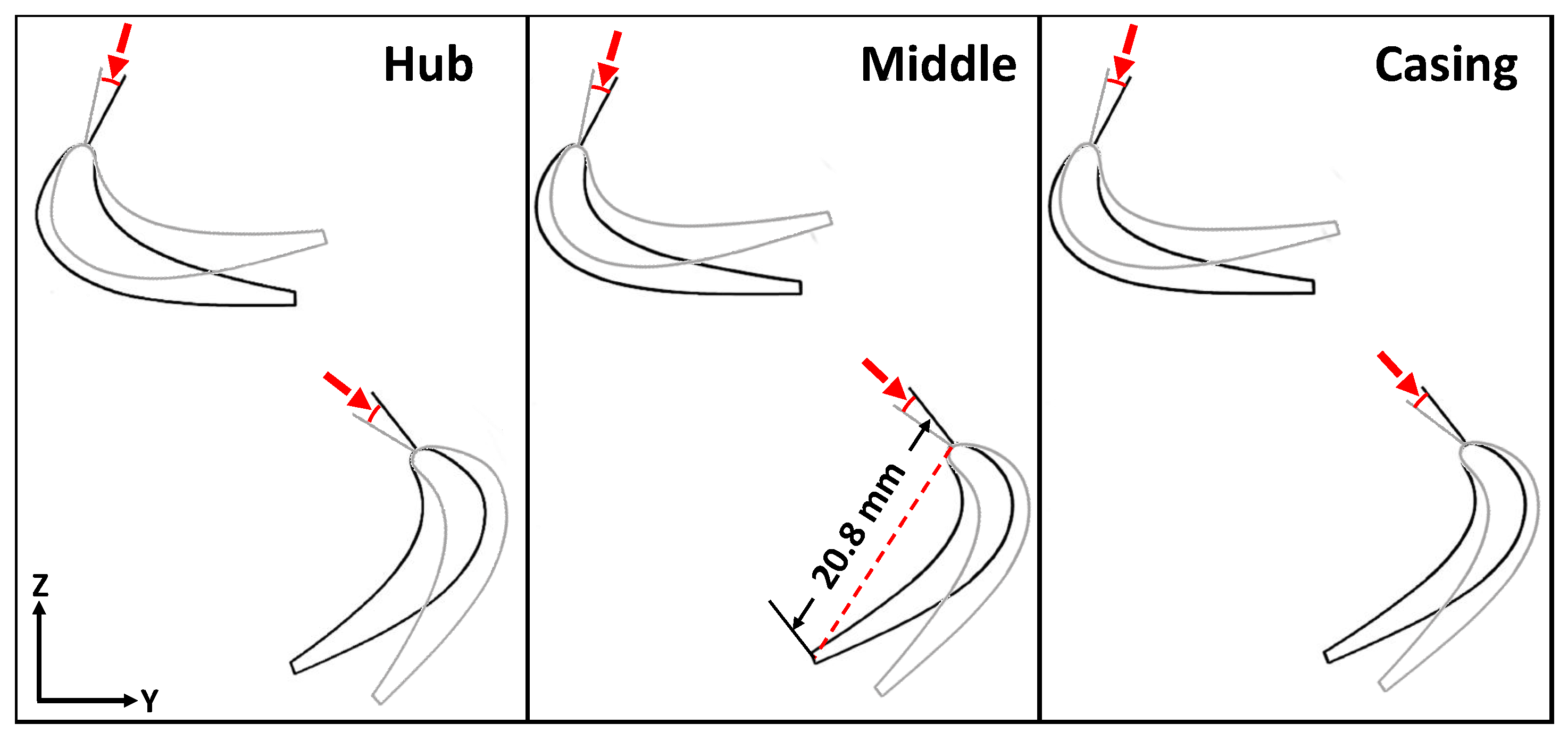
Abstract
:1. Introduction
2. High-Fidelity Modeling of Compressible Flow in a Gas Turbine Stage
2.1. Moving-Domain Finite Element Formulation of Compressible Flows
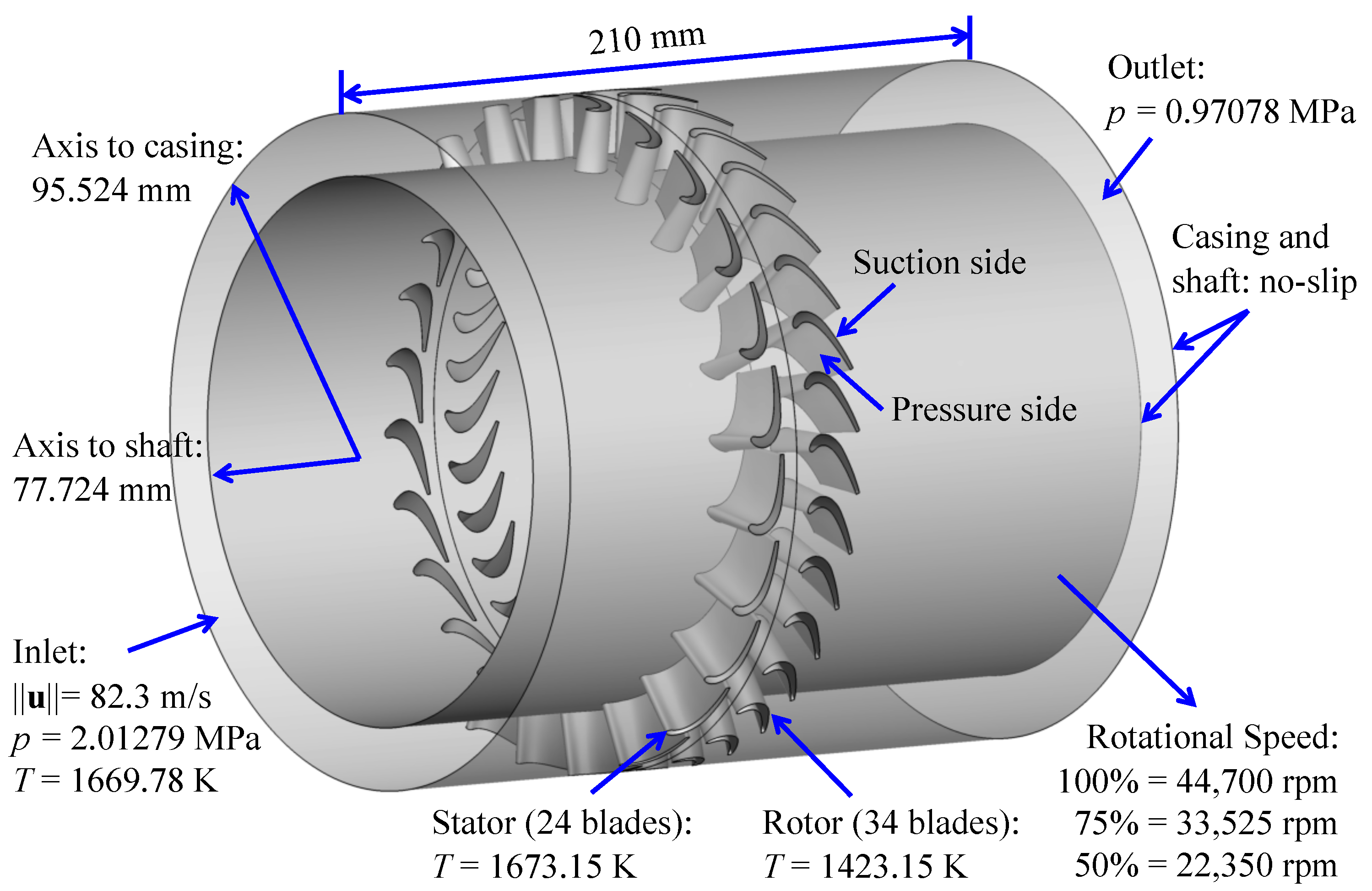
2.2. Model of the Turbine Stage
3. Design Optimization Methodology
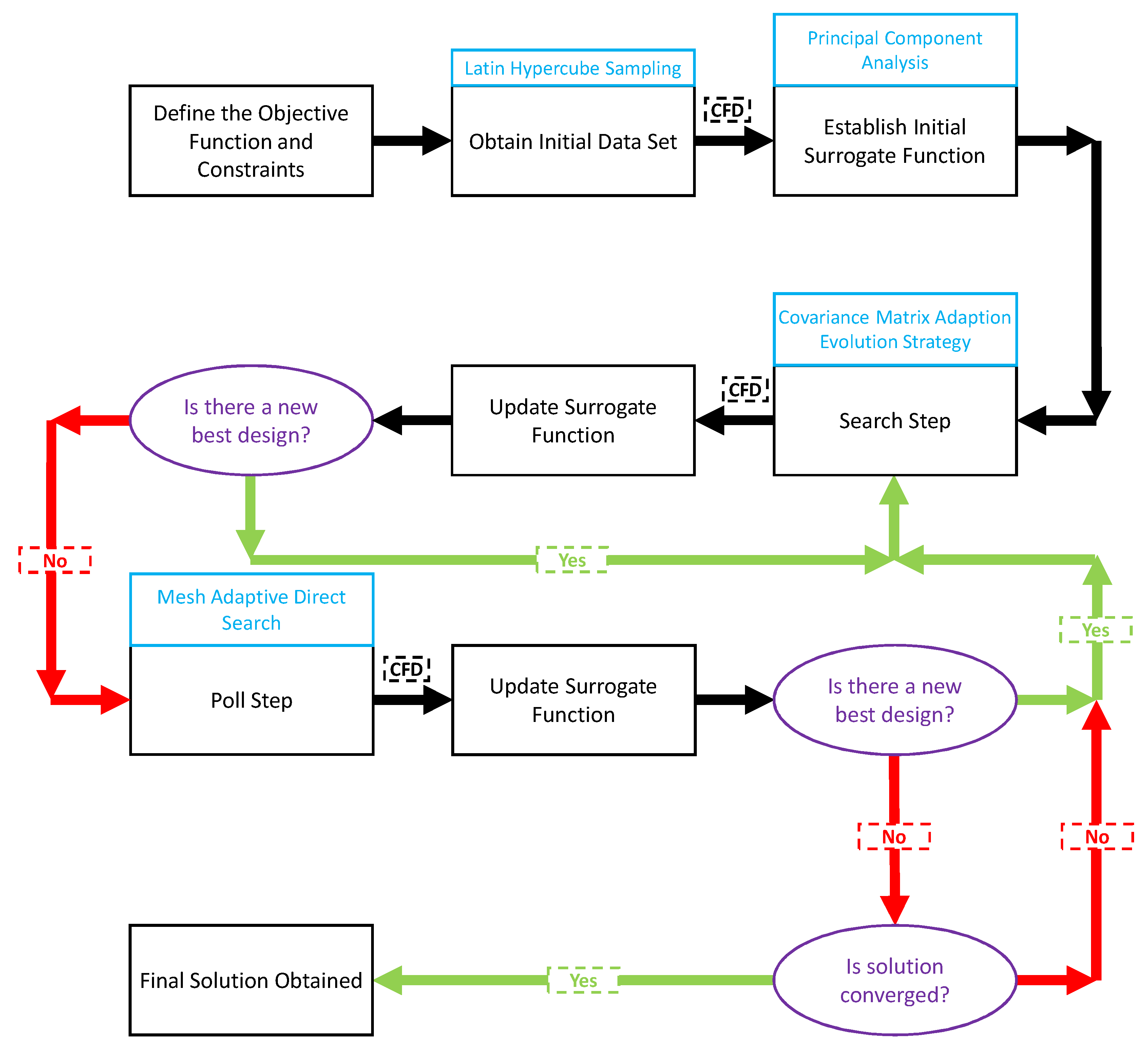
3.1. Surrogate Management Framework
3.2. SMF Modifications for VSGTE Optimization
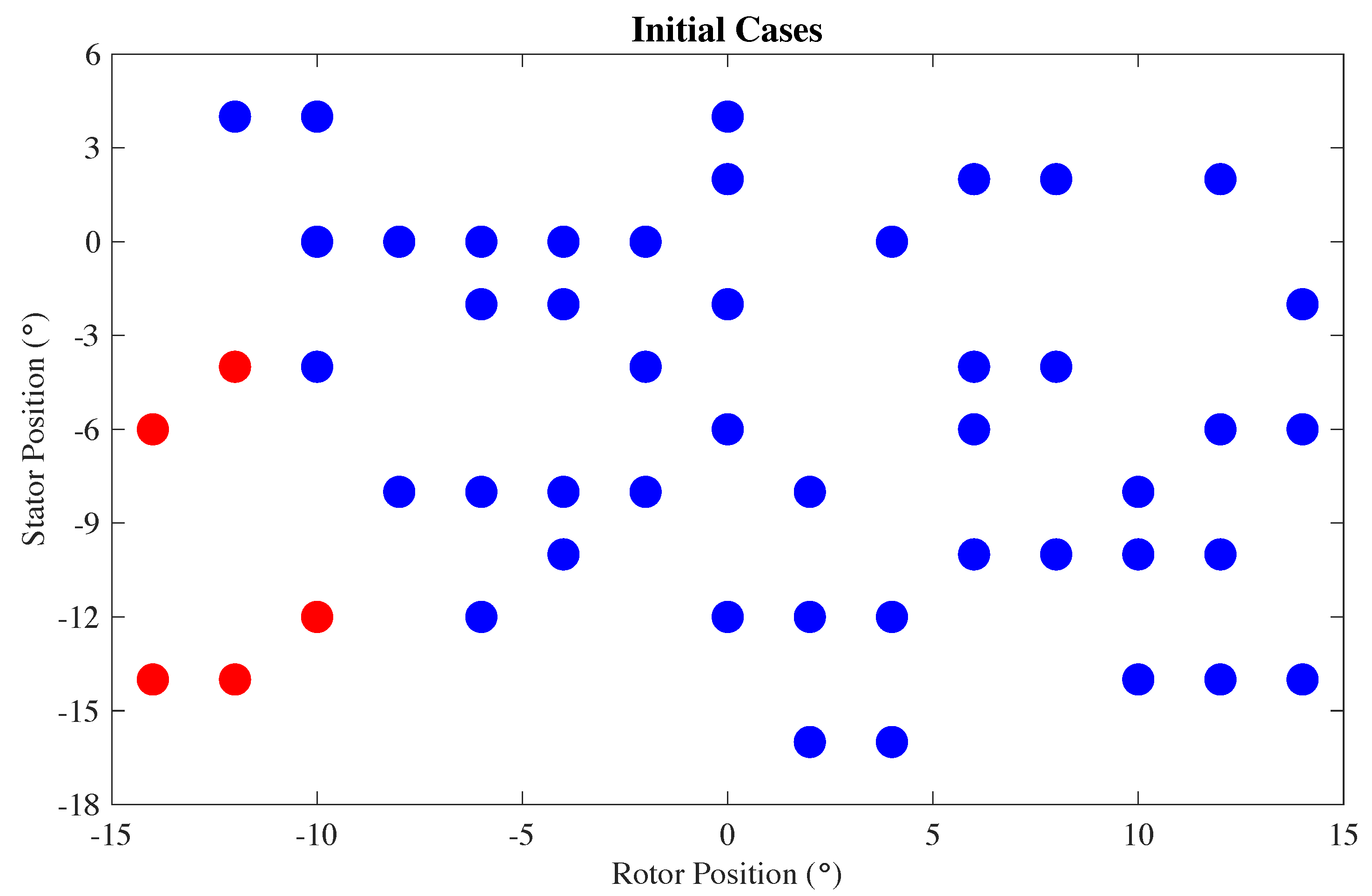
3.3. Design and Analysis Spaces
3.4. Evaluation of Analysis-Space Parameters
3.5. Objective Function and Constraints
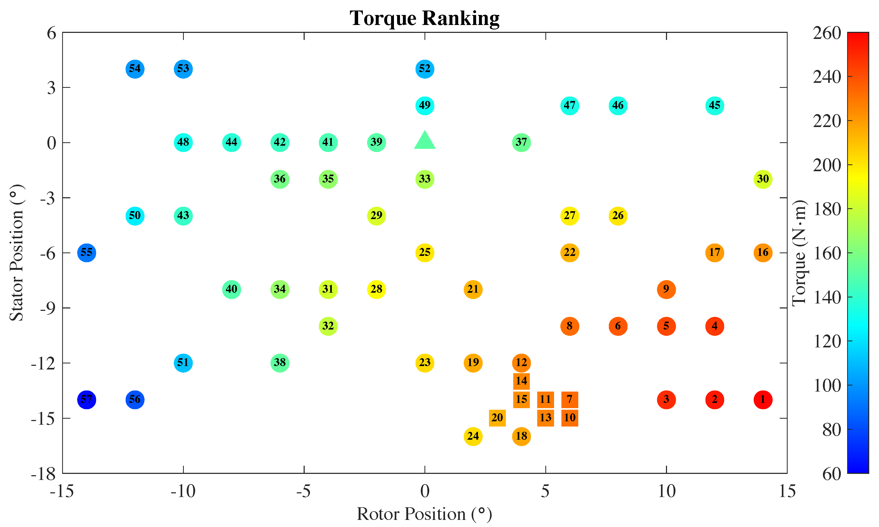
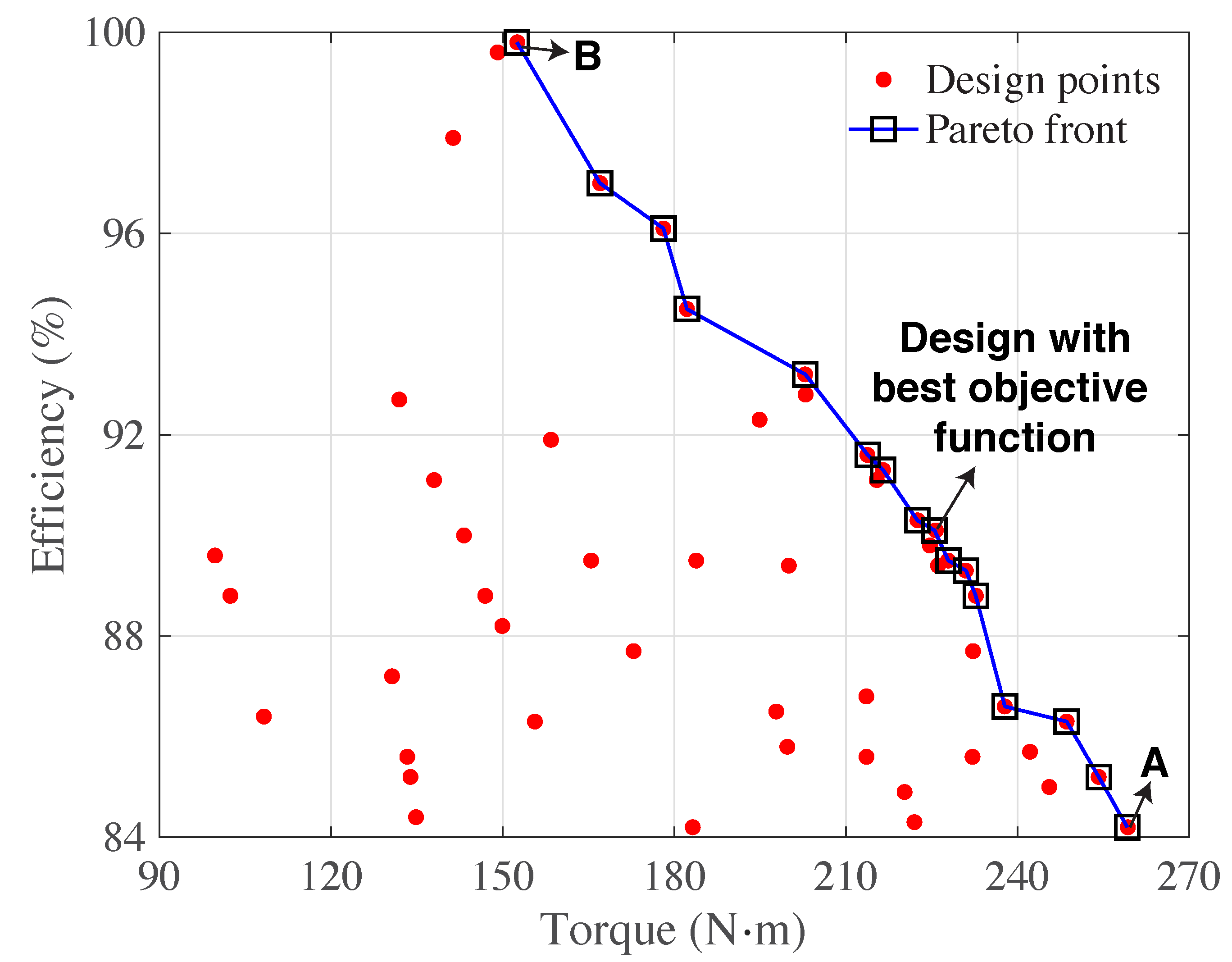
4. Optimization Results
4.1. Convergence of the SMF Algorithm
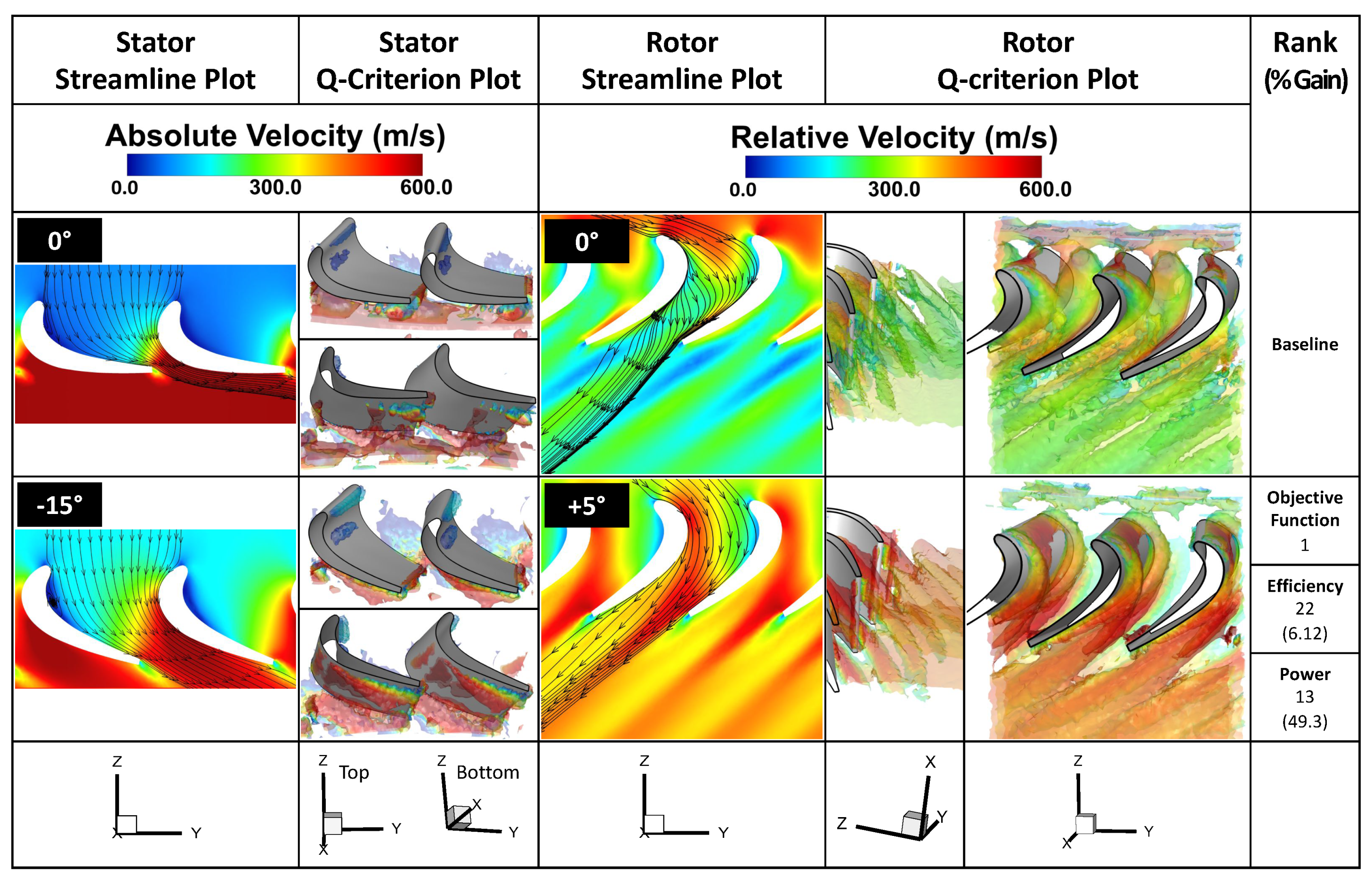
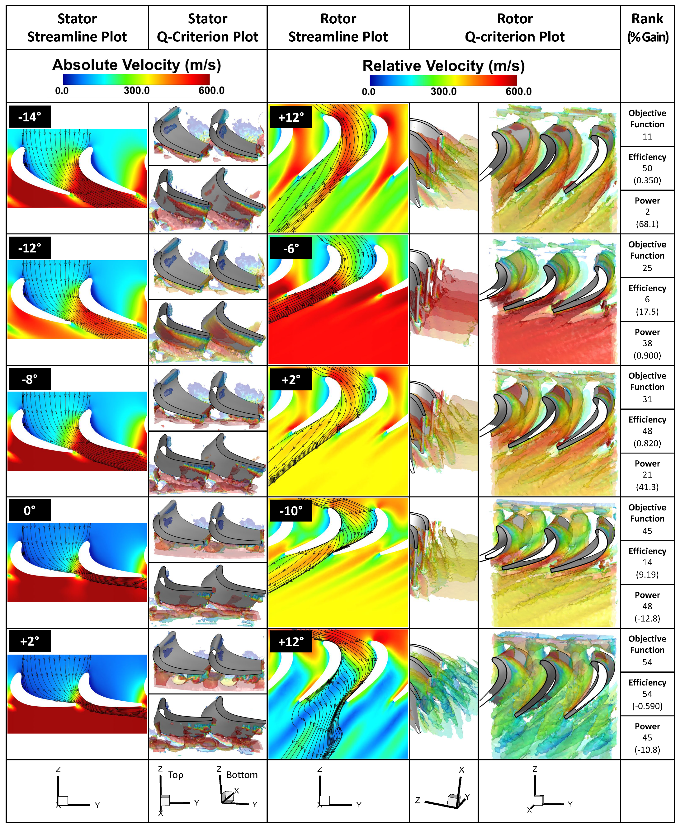
4.2. Flow Analysis
5. Conclusions
Author Contributions
Funding
Acknowledgments
Conflicts of Interest
References
- Welch, G.E. Assessment of aerodynamic challenges of a variable-speed power turbine for large civil tilt-rotor application. In Proceedings of the 66th American Helicopter Society International Annual Forum (AHS Forum 66), Phoenix, AZ, USA, 11–13 May 2010. [Google Scholar]
- Murugan, M.; Booth, D.; Ghoshal, A.; Thurman, D.; Kerner, K. Concept study for adaptive gas turbine rotor blade. Int. J. Eng. Sci. 2015, 4, 10–17. [Google Scholar]
- Murugan, M.; Ghoshal, A.; Xu, F.; Hsu, M.C.; Bazilevs, Y.; Bravo, L.; Kerner, K. Analytical Study of Articulating Turbine Rotor Blade Concept for Improved Off-Design Performance of Gas Turbine Engines. J. Eng. Gas Turbines Power 2017, 139, 102601. [Google Scholar] [CrossRef] [Green Version]
- Grossman, J.; Rubenson, D.; Sollfrey, W.; Steele, B. Vertical Envelopment and the Future Transport Rotorcraft; RAND Corporation: Santa Monica, CA, USA, 2003. [Google Scholar]
- Mcdonald, C.; Wilson, D. The utilization of recuperated and regenerated engine cycles for high-efficiency gas turbines in the 21st century. Appl. Therm. Eng. 1996, 16, 635–653. [Google Scholar] [CrossRef]
- Kozak, N.; Xu, F.; Rajanna, M.R.; Bravo, L.; Murugan, M.; Ghoshal, A.; Bazilevs, Y.; Hsu, M.C. High-fidelity finite element modeling and analysis of adaptive gas turbine stator–rotor flow interaction at off-design conditions. J. Mech. 2020. [Google Scholar] [CrossRef]
- Rajanna, M.R.; Xu, F.; Hsu, M.C.; Bazilevs, Y.; Murugan, M.; Ghoshal, A.; Bravo, L. Optimizing gas-turbine operation using finite-element cfd modeling. In Proceedings of the 2018 Joint Propulsion Conference, Cincinnati, OH, USA, 9–11 July 2018. [Google Scholar]
- Logan, E., Jr.; Roy, R. Handbook of Turbomachinery, 2nd ed.; CRC Press: Boca Raton, FL, USA, 2003. [Google Scholar]
- Booker, A.J.; Dennis, J.E., Jr.; Frank, P.D.; Serafini, D.B.; Torczon, V.; Trosset, M.W. A rigorous framework for optimization of expensive functions by surrogates. Struct. Optim. 1999, 17, 1–13. [Google Scholar] [CrossRef]
- Hansen, N. A CMA-ES for Mixed-Integer Nonlinear Optimization; Technical Report RR-7751; Institut National de Recherche en Informatique et en Automatique: Rocquencourt, France, 2011. [Google Scholar]
- Audet, C.; Dennis, J.E., Jr. Mesh adaptive direct search algorithms for constrained optimization. SIAM J. Optim. 2006, 17, 188–217. [Google Scholar] [CrossRef] [Green Version]
- Benaouali, A.; Kachel, S. A surrogate-based integrated framework for the aerodynamic design optimization of a subsonic wing planform shape. J. Aerosp. Eng. 2018, 232, 872–883. [Google Scholar] [CrossRef]
- Wu, M.C.H.; Kamensky, D.; Wang, C.; Herrema, A.J.; Xu, F.; Pigazzini, M.S.; Verma, A.; Marsden, A.L.; Bazilevs, Y.; Hsu, M.C. Optimizing fluid–structure interaction systems with immersogeometric analysis and surrogate modeling: Application to a hydraulic arresting gear. Comput. Methods Appl. Mech. Eng. 2017, 316, 668–693. [Google Scholar] [CrossRef] [Green Version]
- Long, C.C.; Marsden, A.L.; Bazilevs, Y. Fluid–structure interaction simulation of pulsatile ventricular assist devices. Comput. Mech. 2013, 52, 971–981. [Google Scholar] [CrossRef]
- Verma, A.; Wong, K.; Marsden, A.L. A concurrent implementation of the surrogate management framework with application to cardiovascular shape optimization. Optim. Eng. 2020. [Google Scholar] [CrossRef]
- Hughes, T.J.R.; Tezduyar, T.E. Finite element methods for first-order hyperbolic systems with particular emphasis on the compressible Euler equations. Comput. Methods Appl. Mech. Eng. 1984, 45, 217–284. [Google Scholar] [CrossRef] [Green Version]
- Hughes, T.J.R.; Franca, L.P.; Mallet, M. A new finite element formulation for computational fluid dynamics: I. Symmetric forms of the compressible Euler and Navier-Stokes equations and the second law of thermodynamics. Comput. Methods Appl. Mech. Eng. 1986, 54, 223–234. [Google Scholar] [CrossRef]
- Hughes, T.J.R.; Mallet, M. A new finite element formulation for computational fluid dynamics: III. The generalized streamline operator for multidimensional advective-diffusive systems. Comput. Methods Appl. Mech. Eng. 1986, 58, 305–328. [Google Scholar] [CrossRef]
- Hughes, T.J.R.; Franca, L.P.; Mallet, M. A new finite element formulation for computational fluid dynamics: VI. Convergence analysis of the generalized SUPG formulation for linear time-dependent multi-dimensional advective-diffusive Systems. Comput. Methods Appl. Mech. Eng. 1987, 63, 97–112. [Google Scholar] [CrossRef]
- Le Beau, G.J.; Ray, S.E.; Aliabadi, S.K.; Tezduyar, T.E. SUPG finite element computation of compressible flows with the entropy and conservation variables formulations. Comput. Methods Appl. Mech. Eng. 1993, 104, 397–422. [Google Scholar] [CrossRef]
- Aliabadi, S.K.; Tezduyar, T.E. Space–time finite element computation of compressible flows involving moving boundaries and interfaces. Comput. Methods Appl. Mech. Eng. 1993, 107, 209–223. [Google Scholar] [CrossRef]
- Hauke, G.; Hughes, T.J.R. A unified approach to compressible and incompressible flows. Comput. Methods Appl. Mech. Eng. 1994, 113, 389–396. [Google Scholar] [CrossRef]
- Hauke, G.; Hughes, T.J.R. A comparative study of different sets of variables for solving compressible and incompressible flows. Comput. Methods Appl. Mech. Eng. 1998, 153, 1–44. [Google Scholar] [CrossRef]
- Hauke, G. Simple sabilizing matrices for the computation of compressible flows in primitive variables. Comput. Methods Appl. Mech. Eng. 2001, 190, 6881–6893. [Google Scholar] [CrossRef]
- Hughes, T.J.R.; Scovazzi, G.; Tezduyar, T.E. Stabilized Methods for Compressible Flows. J. Sci. Comput. 2010, 43, 343–368. [Google Scholar] [CrossRef]
- Takizawa, K.; Tezduyar, T.E.; Kanai, T. Porosity models and computational methods for compressible-flow aerodynamics of parachutes with geometric porosity. Math. Model. Methods Appl. Sci. 2017, 27, 771–806. [Google Scholar] [CrossRef]
- Kanai, T.; Takizawa, K.; Tezduyar, T.E.; Tanaka, T.; Hartmann, A. Compressible-flow geometric-porosity modeling and spacecraft parachute computation with isogeometric discretization. Comput. Mech. 2019, 63, 301–321. [Google Scholar] [CrossRef] [Green Version]
- Castorrini, A.; Corsini, A.; Rispoli, F.; Venturini, P.; Takizawa, K.; Tezduyar, T.E. Computational analysis of performance deterioration of a wind turbine blade strip subjected to environmental erosion. Comput. Mech. 2019, 64, 1133–1153. [Google Scholar] [CrossRef]
- Castorrini, A.; Venturini, P.; Corsini, A.; Rispoli, F.; Takizawa, K.; Tezduyar, T.E. Computational Analysis of Particle-Laden-Airflow Erosion and Experimental Verification. Comput. Mech. 2020, 65, 1549–1565. [Google Scholar] [CrossRef] [Green Version]
- Hughes, T.J.R.; Liu, W.K.; Zimmermann, T.K. Lagrangian–Eulerian finite element formulation for incompressible viscous flows. Comput. Methods Appl. Mech. Eng. 1981, 29, 329–349. [Google Scholar] [CrossRef]
- Tezduyar, T.E.; Park, Y.J. Discontinuity capturing finite element formulations for nonlinear convection– diffusion–reaction equations. Comput. Methods Appl. Mech. Eng. 1986, 59, 307–325. [Google Scholar] [CrossRef]
- Hughes, T.J.R.; Mallet, M.; Mizukami, A. A new finite element formulation for computational fluid dynamics: II. Beyond SUPG. Comput. Methods Appl. Mech. Eng. 1986, 54, 341–355. [Google Scholar] [CrossRef]
- Hughes, T.J.R.; Mallet, M. A new finite element formulation for computational fluid dynamics: IV. A discontinuity-capturing operator for multidimensional advective-diffusive systems. Comput. Methods Appl. Mech. Eng. 1986, 58, 329–339. [Google Scholar] [CrossRef]
- Shakib, F.; Hughes, T.J.R.; Johan, Z. A new finite element formulation for computational fluid dynamics: X. The compressible Euler and Navier–Stokes equations. Comput. Methods Appl. Mech. Eng. 1991, 89, 141–219. [Google Scholar] [CrossRef]
- Almeida, R.C.; Galeão, A.C. An adaptive Petrov–Galerkin formulation for the compressible Euler and Navier–Stokes equations. Comput. Methods Appl. Mech. Eng. 1996, 129, 157–176. [Google Scholar] [CrossRef]
- Tezduyar, T.E. Finite element methods for fluid dynamics with moving boundaries and interfaces. In Encyclopedia of Computational Mechanics; Stein, E., Borst, R.D., Hughes, T.J.R., Eds.; Volume 3: Fluids; John Wiley & Sons: Hoboken, NJ, USA, 2004; Chapter 17. [Google Scholar]
- Tezduyar, T.E.; Senga, M. Stabilization and shock-capturing parameters in SUPG formulation of compressible flows. Comput. Methods Appl. Mech. Eng. 2006, 195, 1621–1632. [Google Scholar] [CrossRef]
- Tezduyar, T.E.; Senga, M.; Vicker, D. Computation of inviscid supersonic flows around cylinders and spheres with the SUPG formulation and YZβ shock-capturing. Comput. Mech. 2006, 38, 469–481. [Google Scholar] [CrossRef]
- Tezduyar, T.E.; Senga, M. SUPG finite element computation of inviscid supersonic flows with YZβ shock-capturing. Comput. Fluids 2007, 36, 147–159. [Google Scholar] [CrossRef]
- Rispoli, F.; Saavedra, R.; Corsini, A.; Tezduyar, T.E. Computation of inviscid compressible flows with the V-SGS stabilization and YZβ shock-capturing. Int. J. Numer. Methods Fluids 2007, 54, 695–706. [Google Scholar] [CrossRef]
- Rispoli, F.; Saavedra, R.; Menichini, F.; Tezduyar, T.E. Computation of inviscid supersonic flows around cylinders and spheres with the V-SGS stabilization and YZβ shock-capturing. J. Appl. Mech. 2009, 76, 021209. [Google Scholar] [CrossRef]
- Rispoli, F.; Delibra, G.; Venturini, P.; Corsini, A.; Saavedra, R.; Tezduyar, T.E. Particle tracking and particle–shock interaction in compressible-flow computations with the V-SGS stabilization and YZβ shock-capturing. Comput. Mech. 2015, 55, 1201–1209. [Google Scholar] [CrossRef]
- Takizawa, K.; Tezduyar, T.E.; Otoguro, Y. Stabilization and discontinuity-capturing parameters for space–time flow computations with finite element and isogeometric discretizations. Comput. Mech. 2018, 62, 1169–1186. [Google Scholar] [CrossRef]
- Bazilevs, Y.; Hughes, T.J.R. Weak imposition of Dirichlet boundary conditions in fluid mechanics. Comput. Fluids 2007, 36, 12–26. [Google Scholar] [CrossRef]
- Bazilevs, Y.; Michler, C.; Calo, V.M.; Hughes, T.J.R. Weak Dirichlet boundary conditions for wall-bounded turbulent flows. Comput. Methods Appl. Mech. Eng. 2007, 196, 4853–4862. [Google Scholar] [CrossRef]
- Bazilevs, Y.; Michler, C.; Calo, V.M.; Hughes, T.J.R. Isogeometric variational multiscale modeling of wall-bounded turbulent flows with weakly enforced boundary conditions on unstretched meshes. Comput. Methods Appl. Mech. Eng. 2010, 199, 780–790. [Google Scholar] [CrossRef]
- Bazilevs, Y.; Akkerman, I. Large eddy simulation of turbulent Taylor–Couette flow using isogeometric analysis and the residual-based variational multiscale method. J. Comput. Phys. 2010, 229, 3402–3414. [Google Scholar] [CrossRef]
- Hsu, M.C.; Akkerman, I.; Bazilevs, Y. Wind turbine aerodynamics using ALE–VMS: Validation and the role of weakly enforced boundary conditions. Comput. Mech. 2012, 50, 499–511. [Google Scholar] [CrossRef]
- Bazilevs, Y.; Hughes, T.J.R. NURBS-based isogeometric analysis for the computation of flows about rotating components. Comput. Mech. 2008, 43, 143–150. [Google Scholar] [CrossRef]
- Hsu, M.C.; Akkerman, I.; Bazilevs, Y. Finite element simulation of wind turbine aerodynamics: Validation study using NREL Phase VI experiment. Wind Energy 2014, 17, 461–481. [Google Scholar] [CrossRef]
- Hsu, M.C.; Bazilevs, Y. Fluid–structure interaction modeling of wind turbines: Simulating the full machine. Comput. Mech. 2012, 50, 821–833. [Google Scholar] [CrossRef]
- Terahara, T.; Takizawa, K.; Tezduyar, T.E.; Bazilevs, Y.; Hsu, M.C. Heart Valve Isogeometric Sequentially-Coupled FSI Analysis with the Space–Time Topology Change Method. Comput. Mech. 2020, 65, 1167–1187. [Google Scholar] [CrossRef] [Green Version]
- Terahara, T.; Takizawa, K.; Tezduyar, T.E.; Tsushima, A.; Shiozaki, K. Ventricle-valve-aorta flow analysis with the Space–Time Isogeometric Discretization and Topology Change. Comput. Mech. 2020, 65, 1343–1363. [Google Scholar] [CrossRef] [Green Version]
- Otoguro, Y.; Takizawa, K.; Tezduyar, T.E.; Nagaoka, K.; Avsar, R.; Zhang, Y. Space–Time VMS Flow Analysis of a Turbocharger Turbine with Isogeometric Discretization: Computations with Time-Dependent and Steady-Inflow Representations of the Intake/Exhaust Cycle. Comput. Mech. 2019, 64, 1403–1419. [Google Scholar] [CrossRef] [Green Version]
- Chung, J.; Hulbert, G.M. A time integration algorithm for structural dynamics with improved numerical dissipation: The generalized-α method. J. Appl. Mech. 1993, 60, 371–375. [Google Scholar] [CrossRef]
- Jansen, K.E.; Whiting, C.H.; Hulbert, G.M. A generalized-α method for integrating the filtered Navier-Stokes equations with a stabilized finite element method. Comput. Methods Appl. Mech. Eng. 2000, 190, 305–319. [Google Scholar] [CrossRef]
- Bazilevs, Y.; Calo, V.M.; Hughes, T.J.R.; Zhang, Y. Isogeometric fluid–structure interaction: Theory, algorithms, and computations. Comput. Mech. 2008, 43, 3–37. [Google Scholar] [CrossRef]
- Shakib, F.; Hughes, T.J.R.; Johan, Z. A multi-element group preconditioned GMRES algorithm for nonsymmetric systems arising in finite element analysis. Comput. Methods Appl. Mech. Eng. 1989, 75, 415–456. [Google Scholar] [CrossRef]
- Xu, F.; Moutsanidis, G.; Kamensky, D.; Hsu, M.C.; Murugan, M.; Ghoshal, A.; Bazilevs, Y. Compressible flows on moving domains: Stabilized methods, weakly enforced essential boundary conditions, sliding interfaces, and application to gas-turbine modeling. Comput. Fluids 2017, 158, 201–220. [Google Scholar] [CrossRef] [Green Version]
- Xu, F.; Bazilevs, Y.; Hsu, M.C. Immersogeometric analysis of compressible flows with application to aerodynamic simulation of rotorcraft. Math. Model. Methods Appl. Sci. 2019, 29, 905–938. [Google Scholar] [CrossRef]
- Hsu, M.C.; Wang, C.; Herrema, A.J.; Schillinger, D.; Ghoshal, A.; Bazilevs, Y. An interactive geometry modeling and parametric design platform for isogeometric analysis. Comput. Math. Appl. 2015, 70, 1481–1500. [Google Scholar]
- Huntington, D.E.; Lyrintzis, C.S. Improvements to and limitations of Latin hypercube sampling. Probabilistic Eng. Mech. 1998, 13, 245–253. [Google Scholar] [CrossRef]
- McKay, M.D.; Beckman, R.J.; Conover, W.J. A comparison of three methods for selecting values of input variables in the analysis of output from a computer code. Technometrics 2000, 42, 55–61. [Google Scholar] [CrossRef]
- Hansen, N.; Ostermeier, A. Completely derandomized self-adaptation in evolution strategies. Evol. Comput. 2001, 9, 159–195. [Google Scholar] [CrossRef]
- Murugan, M.; Ghoshal, A.; Bravo, L. Adaptable Articulating Axial-Flow Compressor/Turbine Rotor Blade. U.S. Patent Application 20180066671 A1, 8 March 2018. [Google Scholar]
- Audet, C.; Le Digabel, S.; Tribes, C. The mesh adaptive direct search algorithm for granular and discrete variables. SIAM J. Optim. 2019, 29, 1164–1189. [Google Scholar] [CrossRef] [Green Version]
- Schobeiri, M. Turbomachinery Flow Physics and Dynamic Performance; Springer: Berlin/Heidelberg, Germany, 2005. [Google Scholar]
- Fletcher, R. Practical Methods of Optimization, 2nd ed.; John Wiley & Sons: Chichester, UK, 1987. [Google Scholar]
- Wold, S.; Esbensen, K.; Geladi, P. Principal Component Analysis. Chemom. Intell. Lab. Syst. 1987, 2, 37–52. [Google Scholar] [CrossRef]
- Jeong, J.; Hussain, F. On the identification of a vortex. J. Fluid Mech. 1995, 285, 69–94. [Google Scholar] [CrossRef]


© 2020 by the authors. Licensee MDPI, Basel, Switzerland. This article is an open access article distributed under the terms and conditions of the Creative Commons Attribution (CC BY) license (http://creativecommons.org/licenses/by/4.0/).
Share and Cite
Kozak, N.; Rajanna, M.R.; Wu, M.C.H.; Murugan, M.; Bravo, L.; Ghoshal, A.; Hsu, M.-C.; Bazilevs, Y. Optimizing Gas Turbine Performance Using the Surrogate Management Framework and High-Fidelity Flow Modeling. Energies 2020, 13, 4283. https://doi.org/10.3390/en13174283
Kozak N, Rajanna MR, Wu MCH, Murugan M, Bravo L, Ghoshal A, Hsu M-C, Bazilevs Y. Optimizing Gas Turbine Performance Using the Surrogate Management Framework and High-Fidelity Flow Modeling. Energies. 2020; 13(17):4283. https://doi.org/10.3390/en13174283
Chicago/Turabian StyleKozak, Nikita, Manoj R. Rajanna, Michael C. H. Wu, Muthuvel Murugan, Luis Bravo, Anindya Ghoshal, Ming-Chen Hsu, and Yuri Bazilevs. 2020. "Optimizing Gas Turbine Performance Using the Surrogate Management Framework and High-Fidelity Flow Modeling" Energies 13, no. 17: 4283. https://doi.org/10.3390/en13174283