Smoothed Particle Hydrodynamics Simulation of High Velocity Impact Dynamics of Molten Sand Particles


1
Karlsruhe Institute of Technology, Institute of Thermal Turbomachinery, Kaiserstr. 12, 76131 Karlsruhe, Germany
2
US Army Research Laboratory, Aberdeen Proving Ground, MD 21005, USA
3
Department of Aerospace Engineering, University of Maryland, College Park, MD 20742, USA
*
Author to whom correspondence should be addressed.
†
Current address: Department of Mechanical and Aerospace Engineering, George Washington University, Washington, DC 20052, USA.
Energies 2020, 13(19), 5134; https://doi.org/10.3390/en13195134
Submission received: 14 August 2020
/
Revised: 23 September 2020
/
Accepted: 24 September 2020
/
Published: 2 October 2020
(This article belongs to the Special Issue Advancements in Multiphase Fluid Dynamics in Energy and Propulsion Systems)
Abstract
:Sand ingestion is highly detrimental for gas turbines because it leads to erosion and corrosion of engine components, accelerating material fatigue and contributing to global engine failure. In this paper the high velocity impact of a molten sand particle onto a solid wall is investigated by means of the Smoothed Particles Hydrodynamics method where the three phases are taken into account. Nominal conditions are a 25 m particle composed of molten sand (dynamic viscosity Pa·s) impacting the wall at a velocity of 250 m/s. The influence of different parameters are explored such as the mechanical properties of the molten sand particle (density, viscosity, surface tension), the impact conditions (velocity magnitude, particle size and angle of impact) as well as the particle shape (sphere or cube with different geometrical features impacting the wall). It is found that the particles do not form a lamella during the impact but mostly conserve its initial shape. It is also confirmed that sharp features such as edges lead to a larger normal pressure at the impact location. Correlations to quantify (i) the spread factor, (ii) the maximum and mean impact force and impact pressure and (iii) the slip distance are derived for the first time based on the investigated parameters. The importance of these correlations is that they provide information needed to implement low-order models for studying impact and deposition of molten sand in engineering simulations.
1. Introduction
During mission operations of flying vehicles, gas turbines engines can ingest small solid particles during take-off or hovering, or when flying through a dust storm. The most common types of ingested particulates are volcanic ash, desert sand, dust and salt, in the form of calcia-magnesia-alumino-silicates (CMAS), where the specific composition of particulates often varies with geographical location. When ingested, these solid particles may impact engine components at high velocity, increasing the mechanical fatigue of the protective material and eventually lead to component failure. As particles pass through the engine combustor stage, where the operating temperatures exceed the melting point of sand (1300–1600 C), they change phase. This leads to an increase in deposition onto engine component surfaces and enhances the potential for chemical reactions with the thermal or environmental barrier coating (T/EBC). In addition, when the ingested material sticks to the surface of components, it can lead to a degradation of the flow path, clogging of fuel nozzles or blockage of cooling holes [1]. Even though typical particles separators can remove particles larger than ≈80 m, smaller particles pass through and are entrained into the turbine stage. Extensive use of particle separation systems also negatively impacts the overall system performance due to a reported high loss of inlet pressure and inlet mass flow [2]. To date, contaminated environments remain an enduring challenge for the aviation community, not only in desert regions, but also to enable safer flights near complex megacities and urban canyon environments across the world [3,4].
In order to develop superior protective systems that are resistant to CMAS attack, an integrated computational and experimental approach that leads to predictive models and insights of the interaction physics is essential. Over the last two decades multiple experimental research efforts have focused on developing novel protective materials to improve corrosion resistance to CMAS attack [5,6]. A more detailed understanding of how particles behave when they impact surfaces is needed to guide design of T/EBCs and, for example, to precisely define suitable targets for boundary surface energies and to tailor the surface wettability characteristics. Recently, simulations of CMAS particulates have been conducted to study the dynamics of droplet binary collisions and to characterize the turbulent kinetic energy process [7,8]. The results provide critical information needed for the development of CMAS coalescence and breakup models in coarse-grained sand-laden simulations. Bravo et al. [4] conducted analysis of CMAS particulates and their deposition for transonic flows through a linear cascade of blades and reported the sensitivity to the particle Stokes number. Recently, Singh & Tafti [9] developed a low-order deposition model for sand particles at high temperature based on the sticking probability. The sticking probability includes the effects of impact velocity (magnitude and angle) and temperature of the particle. The researchers took into account the change of state of the material due to the kinetic energy dissipation during the impact. They used their model within LES simulations of the impact of a sand-particle-laden jet on a flat coupon and compared it with the experiment [10], showing a satisfactory agreement. Goshal et al. [3] and Murugan et al. [11] conducted numerical investigations on the impact of spherical and sharp edged particles with Computational Fluid Dynamics (CFD) and a software for nonlinear dynamic impact analysis (LS-DYNA). Among their numerous findings, it was shown that sharp edged particles cause more damage than smooth particles and that the particle residence time was sufficiently high for the sand particle to melt. Jain et al. [12] reported the development of a new particle forcing model and conducted Smoothed Particle Hydrodynamics (SPH) simulations of a molten CMAS sessile droplet and computed the contact angle of the droplet on a Yttria-stabilized zirconia (YSZ) material.
The objective of the present work is to simulate the high-speed impact of a molten sand particle under realistic gas turbine operation conditions with a full multiphase approach based on first principles. To the author’s knowledge, such a study has not been performed previously. The different mechanisms associated with the deposition of impurities on turbine blades depend on the Stokes number of the particles in the flow over the blade surfaces. For small particulates in flows with a Stokes number lower than one, these mechanisms are turbulent diffusion, eddy impaction, Brownian diffusion and thermophorese [1]. For larger particulates, typically larger than ≈10 m in realistic gas turbine operation conditions [13], the Stokes number increases and, in turn, particle deposition is dominated by inertial impaction. The present study focuses on the early phase of inertial impaction. Subsequent phenomena, such as deposition, sticking and chemical reactions are not investigated here, and no correlations for spreading or rebound will be applied. The particle deformation and the evolution of the interface will be computed based on mass and momentum conservation. As this study is a first step, the focus will be on the mechanical outcomes of the impact. The energy equation will be neglected, such that the heating of the particle/TBC due to the dissipation of kinetic energy will not be taken into account. The selected numerical approach is the SPH method. It is a mesh-free Lagrangian method where the discretization is performed by elements which are called particles. These particles are moving at the fluid velocity and carry physical quantities such as pressure, mass, momentum and energy. As a Lagrangian particle method, it inherently takes advection and the corresponding acceleration into account. When simulating multiphase flows, each phase is represented by different particle types (e.g., gas, solid, liquid) featuring different physical properties. All phases are computed with the same formalism. The SPH method was originally developed in the context of astrophysics [14,15]. It is nowadays successfully applied in many fields of fluid mechanics such as free surface flows [16], fluid-structure interactions [17], turbulent flows [18] and compressible flows [19]. In the context of liquid droplet impact on walls, the SPH method was used to investigate the influence of porosity and roughness on sessile droplet spreading [20,21]. The shape of the impinging droplet was investigated [22], and the liquid vaporization was taken into account to study the influence of the wall temperature [23]. The SPH method has also been applied to solid deformation and brittle failure of rocks during impacts [24].
2. Numerical Model
2.1. Method
In the SPH method, any field and its derivative are expressed at a given particle location (subscript a) by an interpolation over its neighbor particles (subscript b) [25]:
where is the volume of the neighbor particles. The term W is a weighting function, referred to as the kernel. It depends on the interparticle distance and a characteristic length scale h (smoothing length). Its role is to promote the influence of closer neighbors (Figure 1, top). Only the neighbors encompassed in the so-called sphere of influence (Figure 1, bottom) whose radius is proportional to h are accounted for in Equation (1).
The kernel used in this study is a quintic spline:
where is the distance between particle a and b normalized by the smoothing length h and is equal to the initial mean particle spacing . The radius of the sphere of influence is . The terms , and are abbreviated by , and in the rest of this work.
We express the motion of the fluid phases (gas and liquid) by the weakly-compressible Navier–Stokes equations. Continuity is formulated using the particle volume and density [26]:
where , the mass of particle a, is a constant. This expression of the density does conserve the mass exactly and eliminates any numerical diffusion of density at phase interfaces [27]. The conservation of linear momentum of particle a is expressed by:
where is the particle velocity and , , and are the forces due to pressure, viscosity, surface tension and gravity, respectively. They are expressed as:
Equation (5a) exhibits a particular type of pressure gradient where the two pressures are summed. This formulation has the advantage of (i) conserving linear momentum locally and (ii) increasing the stability of the simulation. Its counterpart is a high sensitivity of the gradient accuracy on disordered particle lattices [28]. Note that there exists another type of gradient where the two pressures and are subtracted instead of being summed. This type of gradient leads to a better approximation on disordered particle lattices but it does not conserve momentum locally and cancel the stabilizing effect of the background pressure, presented later. The formulation of the viscous term (Equation (5b)) is taken from Cleary [29]. It conserves locally the linear and the angular momentum. The interparticle viscosity is proposed by Szewc et al. [30]:
where is the kinematic viscosity. This formulation, which combines an arithmetic average for the kinematic viscosity and a harmonic average for the density, has previously been shown to feature good stability characteristics, especially for predicting airblast atomization where the shear stress of the light phase is very high [31]. Surface tension (Equation (5c)) is adapted from the Continuum Surface Force (CSF) model [32] following Hu and Adams [27] and Adami et al. [33].
According to the weakly compressible assumption, the pressure at particle a is expressed by the equation of state as originally proposed by Cole [34]:
where , and are the nominal particle density, the polytropic ratio and the background pressure, respectively. Note that the background pressure does not appear in the original formulation Cole [34] but was later added by Colagrossi and Landrini [35] for stability purpose. The artificial speed of sound (c) must satisfy the condition for the weakly compressible assumption, ensuring the density variation to be lower than 1% [36]. Furthermore, it was observed in practice that with the present multiphase formulation and equation of state, two additional conditions need to be imposed. First, it is recommended to have:
in order to improve the numerical stability at the interface between medium 1 and medium 2. When Equation (8) is not satisfied, the computation of the pressure gradient at the phase interface leads to an exaggerated impact of the particle distribution from one medium on the other one. More details can be found in [31]. Second, it is necessary to limit the influence of the background pressure versus the effect of compressibility. This is achieved by keeping the ratios:
as low as possible, where the subscript i refers to the phase. It was observed in practice that a value between 0.01 and 0.2 for is sufficient. For a too low value of , the simulation becomes numerically unstable whereas leads to artificial particle acceleration due to the background pressure which is much larger than the acceleration due to the physics (pressure gradient, viscosity, etc.).
Equation (4) is integrated in time by a predictor–corrector scheme. The time step of the numerical simulation is controlled by convection, viscosity, surface tension and the overall acceleration. It is computed at each iteration step:
where is the magnitude of the particle acceleration and to are constants equal to 0.5, 0.25, 0.25 and 0.5, respectively.
2.2. Geometry
The geometry studied in the present work is illustrated in Figure 2. It consists of a circular plate (the substrate) surrounded by a layer of air. In order to reduce the computational costs, the air layer thickness is limited according to the initial droplet position, and an inlet tube is added for injecting the droplet. At the inlet of this tube a constant air velocity is imposed to represent the air entrained by the droplet. The bulk velocity is set to 10% of the droplet velocity. An outflow condition is imposed on the side of the domain, and a no-slip condition is imposed on the impact plate. At the top of the air layer, a wall with slip boundary condition is set as boundary condition. This choice, i.e., a wall and not an inlet or an outlet is motivated by the fact that the flow above the plate will be mostly radial, thus parallel to the surface of the boundary, which typically leads to numerical instabilities in the case of outlet/inlet boundary conditions. The dimension of the geometries for the validation and real condition cases are reported in Table 1.
2.3. Initial Conditions
The initial conditions of a SPH simulation can greatly affect the results [37]. This was also observed here as explained in the following. In case of the simplest initialization procedure, the particles are placed on a regular grid. Here, the particles were placed on a cylindrical grid, which describes concentric circles separated by in the radial and azimuthal directions. With such an initial condition, preliminary tests showed that the impacts of viscous liquid ( Pa·s) led to splash in an hexagonal shape, which was not confirmed by any experiment. The discrepancy was attributed to the initial particle location. Therefore, a specific procedure was developed and applied to overcome this numerical artifact. In a first simulation, the domain was filled in with air particles only and flushed with a high velocity from the inlet tube. Second, the inlet velocity was set to zero, and the simulation was run for a few time steps to relax the pressure gradients due to the high velocity flushing. After this step, the particles inside the domain are not aligned on a regular lattice but randomly packed. By this initial particle arrangement, the unwanted effect of the pressure term according to the equation of state (Equation (7)) could by minimized. Finally, the particles located at the prescribed droplet initial locations were given the appropriate liquid properties and the initial droplet velocity.
3. Validation with a Liquid Droplet
In this section the numerical method is validated against a reference experiment [38] with viscous liquids to assess the fidelity of the numerical model for low Reynolds number impacts. Note that even with large viscosity liquids, the Reynolds number differs by one order of magnitude between the validation experiment (Re ) and the real conditions (Re ). However, these conditions always represent the same regime of laminar flow. Moreover, as it will be confirmed later, the very high viscosity of molten sand is expected to strongly limit the deformation of the sand particle. It is thus expected that the particle will not splash nor be disrupted into ligaments and that the spread will be small. Therefore, we focus in this part of the study on the early phases of the impact where the liquid spreads on the substrate.
3.1. Phenomenology and Scaling of the Early Phase
The early phases of the impact on a dry cold surface are described in the literature as follows. When the distance between the droplet and the surface tends to zero, the flow in between can be considered as a lubrication flow, and the pressure will rise locally, leading to the deformation of the droplet. Air can even be entrapped, generating tiny bubbles inside the liquid [39]. Then the droplet continues to deform as it spills on the substrate. In this phase, the evolution of the droplet deformation and the surface covered by the liquid is mainly driven by the initial diameter, the velocity and the shape of the droplet. Thus, it is called the kinematic phase where the surface covered by the liquid is roughly equal to the surface given by cutting a sphere by a plane at the location at the wall. If the kinetic energy is not fully dissipated during this phase, the liquid will start to be spilled over the substrate. In this case, the phenomenon is controlled not only by kinetic energy but also by viscosity and the wetting condition of the system (surface tension and surface roughness) which is typically quantified by the contact angle. It is very unlikely that a molten sand particle impacting a turbine blade will reach this phase, which will be corroborated by the numerical simulation.
The main quantity to be investigated in the present study is the liquid surface in contact with the substrate, which is discussed in terms of the spread factor. This corresponds to the nondimensional equivalent diameter of the contact surface:
where is the diameter of the droplet prior to the impact, and is the liquid surface in contact with the substrate. In the context of turbine blade impaction by molten sand particle, the contact surface is important because it governs the chemical reactions between CMAS and TBC. Therefore, the spread factor will be investigated in the following. The transient of the early phase is expressed with respect to the nondimensional time . During the kinematic phase, the spread factor is reported to evolve as with a close to 0.5.
3.2. Results
Five test cases were investigated. One was used for qualitative comparison and four for quantitative validation. These are summarized in Table 2. The cases contains approximately 4.7 millions particles and they were run on 125 cores for 150,000 time steps, amounting to 12 ms of physical time. For Case 1 to Case 4, the initiation of the solution was generated according to the procedure described in Section 2.3.
The time series depicted in Figure 3 shows side by side images from the experiments in [38] (top) and the corresponding simulations (bottom). Case 0 was selected for a first qualitative comparison. The droplet surface of the numerical simulation was extracted using the -shape algorithm [40]. An extensive description of our workflow for postprocessing was presented previously [31]. The numerical simulation is found to be in good agreement with the experiment in terms of overall shape and spilled surface. However, it does not correctly capture the rim forming at the front of the lamella, which is attributed to the too coarse spatial resolution of the simulations. In the scope of our study, as the lamella is very unlikely to form during the impact, no rim is to be expected. Therefore, the absence of this structure from the simulation is not detrimental for the validity of the results. One can observe some dispersed lumps of liquid at the periphery of the main region of fluid, especially at the two last time steps (t = 1.31 and 2.27 ms). These are due to the slight numerical instabilities arising on the phase interface during the early phase of the impact. Due to the rapid deformation of the particle lattice in the vicinity of the interface, some liquid particles are ejected outwards and eventually impact the substrate at larger radii. As it represents a negligible volume compared to the total liquid volume, this effect can be neglected in the evaluation of the spread factor.
The pressure was averaged over the symmetry axis of the droplet. It is shown in Figure 4 for early phases of the impact. For , a checkerboard pattern is observed, which then relaxes and disappears at . This pattern is typical for a weakly-compressible SPH simulation initialized with regularly distributed particles. Note that only Case 0 was initialized in this manner. The same field was checked on Case 1 (not depicted here) which was initialized with the procedure described in Section 2.3. In this case, the checkerboard pattern was not visible, which corroborates the fact that the checkerboard pattern is due to the initialization. However, vertical stripes were visible up to , highlighting spurious pressure fluctuations which are typical with weakly-compressible SPH. As the pressure field shows oscillations in the early phase, the overall impact pressure will be then computed in terms of momentum time variation, as detailed later.
For Case 1 to Case 4, the transient of the spread factor was monitored and compared to the experiment. To monitor the transient, it is first necessary to determine the time of impact, which may be a large source of uncertainty in experiments [38]. To extract this incident from the simulations, we monitored the time step where at least one SPH particle is located closer than to the wall. The spread factor was extracted by two means, illustrated in Figure 5. In the first method, the coordinates of the liquid volume in contact with the substrate are expressed in the local cylindrical coordinate system centered at the impact location, and the volume is cut into 360 sectors. In each sector, the particle of maximum radius is selected. The spread factor is computed as the surface of a disk whose radius is equal to the ensemble average of all . In the second method, the contact surface is defined as the volume of liquid between and divided by . In the present case, is set to the inter particle distance . The first method is valid only for a normal impact leading to a symmetrical spreading, whereas the second method can be used for any kind of impact resulting in a lamella of an arbitrary shape.
The spreading computed with the two methods is compared to the experiment in Figure 6. It corresponds to the kinematic and the spreading phases. For all four cases, the spreading computed with method 1 is in good agreement with the experiment. The results given by the second method show a mean deviation of less than 6% for all cases except for Case 3 where it is 10%. We consider this deviation as acceptable, and therefore we will use the second method for the the study of realistic impact scenarios.
The close agreement of the simulated and experimental results shown in Figure 6 indicate that both the kinematic and the spreading phases are correctly predicted. While the former was not a major challenge because it just required proper implementation of conservation of linear momentum and volume, the latter is a promising achievement. It demonstrates that the relative contributions of surface tension, viscosity and wall shear stress are correctly predicted.
4. Application to Realistic Operating Conditions
In this section, the numerical model is applied to real conditions of molten sand particles impacting gas turbine blades. The parameters of the reference case are given in Table 3. Sand particles can exhibit a smooth surface, edges with sharp angles and even corners. Therefore, spherical particles and cubic particles with different orientations to the substrate were investigated.
We consider here molten sand particles with a diameter of 25 m impacting on a solid and nondeformable wall with a velocity of 250 m/s. The mechanical properties are similar to the ones in [12]. The density is 2665 kg/m. The sand particle temperature is estimated to be 1300 C, leading to a viscosity of 11 Pa·s. The surface tension is set to 0.4 kg/s. Air properties were taken at a temperature of 1300 C and 30 bar, leading to a density of 10 kg/m and a viscosity of Pa·s.The large viscosity and large velocity represent an atypical configuration characterized by a very small Reynolds number and a very large Weber number at the same time. This suggests a hierarchy of physics such as surface tension ≪ inertia ≪ viscosity. The surface tension is thus expected to play a negligible role, which will be confirmed subsequently.
The change of temperature of the particle due to the dissipation of kinetic energy can be estimated by considering that only the sand particle is heated, leading to where is the heat capacity of sand. In our conditions ( J/K/kg), K, which can be be significant for the viscosity, as shown in Table 2 from [42]. However, in our parametric study, we investigate a variation up to of each parameter, including viscosity. Therefore, the maximum decrease of viscosity during the impact is taken into account in the parametric study. Concerning the practical conditions of stability (Equations (8) and (9)), the values selected for the speed of sound in air and in molten sand are 5000 and 2500 m/s, respectively. This leads to a ratio of 0.015, and . Although R should be close to one, no numerical instability was observed in the simulation. This is attributed to the large viscosity of the molten sand, leading to a slow deformation of the particle lattice and hence a not too strong source term in the computation of the pressure gradient.
The dimensions of the domain are given in Table 1 and the simulations were initialized as explained in Section 2.3. The domain contains approximately 1.3 million particles and was run over 125 cores for a wall time of 2 h, achieving 30,000 time steps. This leads to a computational cost of 250 CPUhour to simulate 1 microsecond of physical time. The molten sand particle is composed of ≈65,000 particles. Because non-normal impacts were also investigated, the spreading may be nonaxisymmetrical and thus, it was estimated based on the volume in contact with the substrate (method 2).
The outcome of impact is illustrated in Figure 7 for a spherical particle and for a cubic particle impacting the surface at three different orientations. The particle are colored by the height (i.e., the z-coordinate) in yellow-green shades, and the particles in contact with the wall are marked in white. First, no spreading of the lamella is observed, and the particles conserve most of their initial shape. Second, when the particle is cubic, its final deformation depends on the orientation during the impact on the wall. Face impact leads to a very small deformation, whereas corner impact will lead to a strong deformation of the bottom part of the particle. The quantitative results to be presented in the following will demonstrate that the contact surface at the end of the impact is weakly dependent on the particle orientation.
4.1. Influence of Impact Conditions of a Spherical Particle during Normal Impact
First, the influence of mechanical properties as well as the magnitude of the velocity are investigated for the case of a normal impact of a spherical particle. The dimensional parameters were varied to −50%, −20%, 20% and 50% of the reference values as listed in Table 3, leading to a total of 21 different simulations. In the following, different physical quantities will be extracted and plotted versus time. The nondimensional spreading diameter is computed from the volume in contact with the substrate as given by Equation (11) where is the surface of the particle in contact with the substrate. Two different nondimensional times are used:
where is the normal component of the velocity. The nondimensional total force exerted on the substrate by the particle is computed from the nondimensional time derivative of the nondimensional particle momentum such as:
where the subscript i refers to the normal (N) or the tangential (T) component of the velocity. The term is expressed as the summation of the momentum of each numerical particle normalized by the initial momentum component:
where the summation (subscript b) is performed on all the numerical particles that make up the sand grain. Since no splashing was observed, the mass of the sand grain can be considered constant during the impact. In addition, each numerical particle of molten sand has exactly the same mass, thus can be taken out of the summation and , being the number of numerical particle composing the sand grain. It follows that:
where the operator refers to the ensemble average over the numerical particles of the sand grain. Substituting Equation (15) in Equation (13) and expressing the nondimensional time by its dimensional counterpart leads to:
The appearance of two different scaling velocities in Equation (16) is justified by the fact that one stems from the nondimensional time where the total velocity is used and the other stems from the nondimensional velocity, where the consideration of the velocity component (normal or tangential) is important. The necessity of this choice will be justified when discussing oblique impacts in Section 4.4. The nondimensional contact pressure is estimated in the same manner by dividing the force by the contact surface:
The computed influence of the sand particle diameter on the evolution of , and is shown in Figure 8 Left. First we describe the general shape of the curves. increases approximately with because the impact ends in the middle of the kinematic phase as the kinetic energy is completely dissipated by the large viscosity of the molten sand. The normalized force exerted on the substrate shows a maximum at , and the maximum normalized pressure is obtained at . Globally, the particle diameter has a weak influence on the normalized quantities, except for a slight decrease of the final spread with and larger and earlier peak of with larger . The normal velocity (Figure 8, right) has a stronger effect on the normalized quantities.
The influence of the viscosity and density is shown in Figure 9. The global shape of the curves is kept similar except for kg/m (Figure 9, right) where decreases and becomes negative at the same time, indicating the first phase of a rebound. However, the sand particle does not detach from the surface, as does not decrease to zero. Finally, the variation of the surface tension from −50% to +50% of the reference value led to exactly the same transients. This confirms the very weak influence of the surface tension, and thus this transient is not shown.
4.2. Correlation Characterizing the Normal Impact
The smooth and monotonic variation of the curves from Figure 8 and Figure 9 suggest simple correlations between the output values of interest (, and ) and the physical parameters (, , and ). However, we are not interested in finding correlations for the whole transient signal but we focus on characteristic values of the transient. Therefore, we define scalar quantities for each output value that we correlate to the input parameters. For , we define the final spread factor and the time where the spread factor reaches 95% of its final value. For and , we define its peak value (where or ), the time when the peak value is obtained, the time when the value decreases to 5% of the peak and the time average between and . For each quantity, we fit the coefficients of the function:
where the normalizing parameters and the results of the fitting are given in Table 4. To visualize the accuracy of these correlations, we plot the results of Equation (18) versus the values extracted from the simulations in Figure 10, where the black plain line represents and the grey dashed lines represent a variation of 5%. For most quantities the correlations are within the limits of accuracy, except for , and . In the case of , it seems that an additive constant could lead to a better fitting while in the case of it seems rather constant around 0.07. Apart from these three, the correlations (Equation (18) with Table 4) could be embedded in large scale simulations.
4.3. Influence of the Particle Shape
The impact of a cubic particle was investigated for different orientations towards the wall, thus leading to a study of the impact of different geometrical features summarized in Figure 7. In Figure 11 Left we compare when the cubic particle impacts the wall with a face, an edge and a corner, to a sphere of the same volume. The first striking element in Figure 11 Left is that the final spread is almost independent of the type of geometrical feature impacting on the wall. Concerning the transients, it is found that the spread increases faster when the initial impact surface increases. The extreme cases are on one hand the cube corner where ideally the impact starts by a infinitesimal point touching the wall, and on the other hand the cube face where the initial spread is close to the final spread. Concerning the force exerted onto the wall, the shape of the curves is similar, and only the values of the peak and its temporal evolution depend on the geometrical features. This is due to the deformation of the particle during the impact. With a low amount of matter in the direction of the impact (e.g., the corner impact), the particle deformation is larger and occurs over a longer time, thus leading to lower strain and hence a lower force. To the contrary with a face impact, the amount of matter relative to the projected area is maximal (square impact surface vs. the same projected square area), so that the deformation is minimum, thus leading to a large impact force. The curve of the pressure has a similar shape except for the corner impact where peaks in the very early phase of the impact. This peak can be explained by the very small surface of the corner, which results in a high surface pressure of the predictions. Thus, in order to avoid a too large numerical uncertainty, the contact surface was taken into account in Equation (17) only when it contains more than three SPH particles. The presence of the peak of for the corner corroborates the findings from [3,11] stating that sharp particles are more deleterious for the blade than smoother ones. Indeed for the same particle deceleration, the local pressure on the substrate is much larger for sharp particles which will lead to an augmented erosion. For the three other geometrical features, the peak of the pressure appears sooner than the peak of force, as for the results of Section 4.1.
The transients for the different cube orientations considered are shown in Figure 11 Right. The orientations are identified by the rotation angles (in degree) of the cube around the axes defining the plane of the substrate passing by the cube center. With this nomenclature, , and represent an impact with a face, an edge and a corner. The same trends as in Figure 11 Left are visible: the final is roughly similar with a mean value around 0.811, and the evolution of the transient is faster when the matter contained in the direction of the impact is larger. The shape of normal force is also regular with different peak locations in (). For the pressure, a peak at the early phase appears for small initial contact surfaces such as the cases , and .
4.4. Oblique Impacts for Spherical and Cubic Particles
The influence of the angle of impact is investigated in this section. For the spherical particle, angles of 0, 15, 30, 45, 60 and 75 were investigated while the cubic particle impacts were studied for angles of 0, 45, 60 and 75, with different orientations, as sketched in Figure 12.
For oblique impacts the tangential component of the velocity is nonzero. Therefore, the tangential component of the force and pressure exerted on the substrate can be studied. In the following we will drop the investigation of the force during impact and focus on the pressure. The tangential component of the pressure is referred to as the shear stress . It is recalled that (resp. ) is normalized by the total velocity (resp. normal velocity ) whereas normal (resp. tangential) forces and pressures are normalized by the normal (resp. tangential) component of the velocity.
In case of an oblique impact, the particle may slip along the substrate, until the kinetic energy corresponding to the tangential velocity component is dissipated by the friction at the interface. Thus, the final location of the particle is different from the impact location. In the following, the distance L between both locations is referred to as the slip and it is labeled in its nondimensional form as:
The arbitrary representation of the nondimensional slip in Equation (19) is motivated by the results to be presented in the following.
The transients of the oblique impact for the sphere are shown in Figure 13. It is found that the curves of and match well when they are plotted versus instead of . The final value of is for while the final slip is for and for . Concerning the normal pressure, the scaling given by Equation (17) provides a satisfactory constant peak value of at . The negative pressure for indicates the first stage of rebound, even though the particle stays always in contact with the substrate. The peak of the shear stress decreases monotonically from six to three and occurs at various times between and 0.15. For angles between 15 and 75, the following correlation for the peak of is proposed:
with in degree.
Figure 14 depicts the transients of an oblique impact of a cube face at different impact angles. The local minima of shows a tipping, when the cube rolls from one face to the next one. Therefore, for the cube has rolled over two times and is completing the third tip at . The roll overs are also visible in the history of indicated by a negative normal pressure. The peaks of normal and tangential pressure decrease monotonically with an increasing impact angle, thus correlations are proposed:
for between 45 and 75.
For the edge impacts (Figure 15 and Figure 16), the curve of suggests that the cube is more likely to roll over when the edge is aligned perpendicular to the velocity. This can be explained geometrically by the fact that at the early phase of the impact, the edge in contact with the wall acts as a tipping line for the cube. The curves of the normal pressure and the shear rate collapse on each other for the perpendicular edge impact (Figure 15), confirming the appropriate scaling, whereas they are slightly stretched in time for the parallel edge impact (Figure 16). In both types of impact, the peak of and are between 12 and 15, and between 3.8 and 4.9, respectively. The curve of sand particle slip shows a roughly similar increase for all cases of both types of impact up to . Afterwards, the final values are confined to a regime between 0.4 and 0.7.
The corner impact was investigated for different oblique impact angles. Results of the transients are shown in Figure 17, where a roll over is observed for . The final spread and slip are approximately independent of the impact angle with and . The evolution of and is not monotonic with , thus no correlations are proposed.
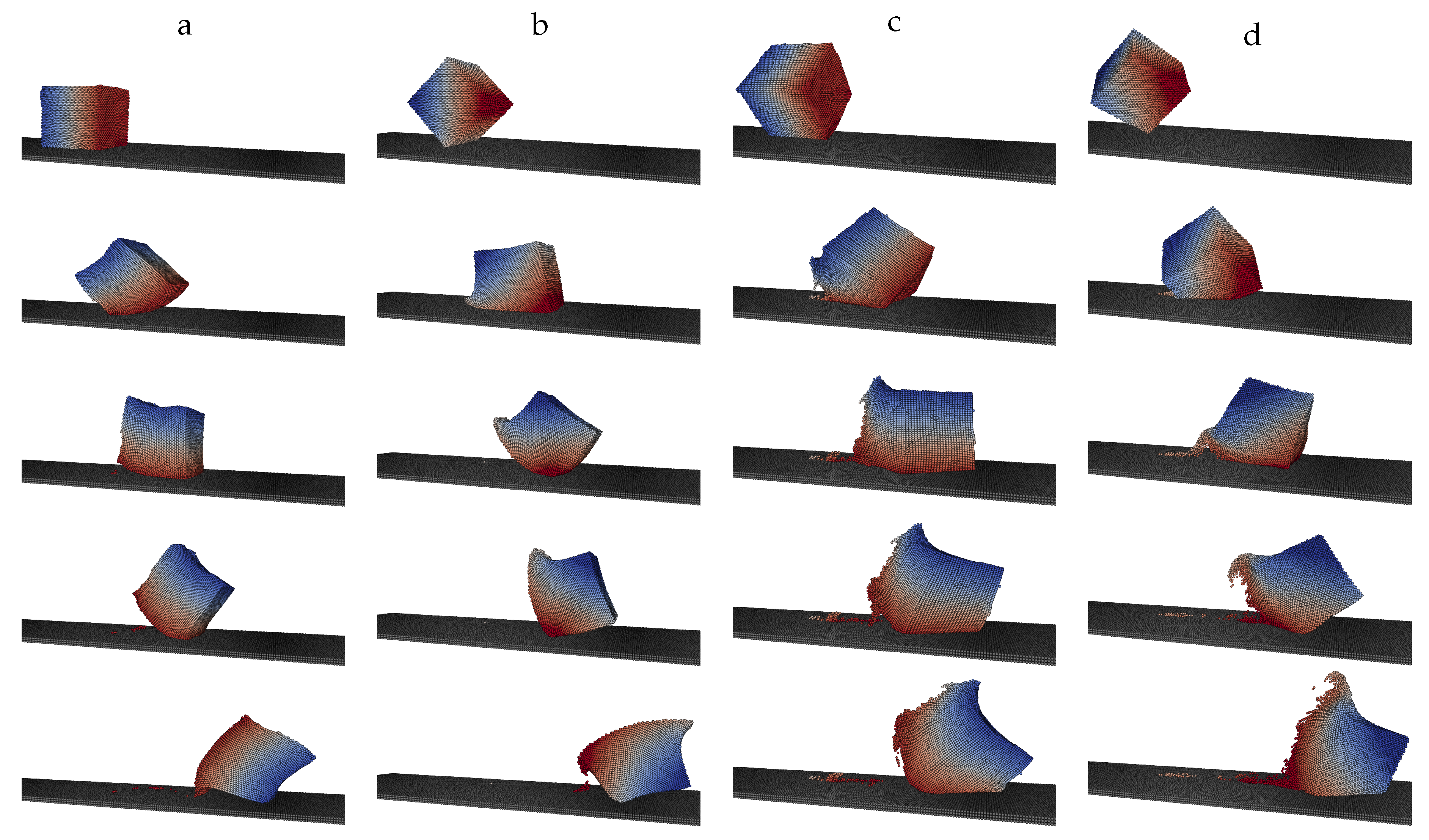
It was seen that for large impact angle, the particle is suspected to roll on the substrate. Time series of cubic particles for an oblique impact of is presented in Figure 18 where the particle are colored by their unique identity tag. The time step between two snapshots is approximately 0.14 s and the last snapshot corresponds to the end of the simulation when the particle has stopped rolling (≈1.5 s after impact). Globally, as for a normal impact, particle deformation is larger when the amount of material touching the substrate is lower. Hence, a face impact (e.g., Figure 12a) weakly deforms the particle, whereas a corner impact (e.g., Figure 12d) creates a tail-like protuberance on the particle. The difference in the deformation has an influence on the number of particles deposited on the surface. When the particle is more deformed during the impact, it is more prone to deposit material on the substrate. Please note that since no microscopic interaction (e.g., chemical bounds, adsorption) between the sand and the substrate are modeled, the number of numerical particles deposited is not sufficient to quantify the mass deposition on the surface. In all cases, the particle has rolled over half a turn, which corresponds to three faces in contact with the substrate, i.e., approximately 50% of particle surface has touched the substrate at the end of the impact.
5. Conclusions
In this paper the high velocity impact of a molten sand particle (approximated as a very viscous liquid) of different shapes on a plane, solid substrate was investigated by means of the SPH method. The method was validated against experiments with impacts of water, glycerin and silicone oil droplets. By analyzing nondimensional quantities of real operating-condition impacts, the viscosity and the inertia of the sand particles were shown to be the governing physical quantities driving the impact scenario. Due to the high viscosity of molten sand, no spreading of lamella were observed; however, partial deformation of the molten particles was observed.
A series of simulations were performed varying particle mechanical properties as well as the impact velocity and the particle diameter by −50%, −20%, 20% and 50% of the reference value. From these results, correlations were derived which characterize the spread factor, the distance to impact and the maximum forces and pressures depending on many operating parameters and mechanical properties of the molten sand. Moreover, scaling laws were proposed in order to increase the applicability of the correlations.
Investigation of the effect of the particle shape under normal impact showed that only the transients are affected by the shape but not the final spread. Concerning the influence of the impact angle , for , all nonspherical particles were found to roll over on the substrate surface before reaching the final position at higher impact angles.
Author Contributions
Conceptualization, G.C. and L.B.; methodology, G.C. and R.K.; validation, G.C.; formal analysis, G.C.; investigation, G.C.; resources, L.B., R.K. and H.-J.B.; writing—original draft preparation, G.C.; writing—review and editing, L.B., A.F. and R.K.; visualization, G.C.; supervision, L.B. and A.F.; project administration, L.B. and A.F.; funding acquisition, R.K. and H.-J.B. All authors have read and agreed to the published version of the manuscript.
Funding
This research was partly funded by the Helmholtz Association of German Research Centres (HGF) (Grant: 34.14.02). The simulations were performed on the computational resource ForHLR Phase II funded by the Ministry of Science, Research and the Arts Baden-Württemberg and DFG (“Deutsche Forschungsgemeinschaft”).
Conflicts of Interest
The authors declare no conflict of interest.
Abbreviations
The following abbreviations are used in this manuscript:
| CFD | Computational Fluid Dynamics |
| CMAS | Calcium-Magnesium-Aluminosilicate |
| LES | Large Eddy Simulation |
| SPH | Smoothed Particle Hydrodynamics |
| T/EBC | Thermal/Environmental Blade Coating |
References
- Hamed, A.; Tabakoff, W.C.; Wenglarz, R. Erosion and Deposition in Turbomachinery. J. Propuls. Power 2006, 22, 350–360. [Google Scholar] [CrossRef] [Green Version]
- Filippone, A.; Bojdo, N. Turboshaft engine air particle separation. Prog. Aerosp. Sci. 2010, 46. [Google Scholar] [CrossRef]
- Ghoshal, A.; Murugan, M.; Walock, M.J.; Nieto, A.; Barnett, B.D.; Pepi, M.S.; Swab, J.J.; Zhu, D.; Kerner, K.A.; Rowe, C.R.; et al. Molten Particulate Impact on Tailored Thermal Barrier Coatings for Gas Turbine Engine. J. Eng. Gas Turbines Power 2018, 140. [Google Scholar] [CrossRef]
- Bravo, L.; Jain, N.; Khare, P.; Murugan, M.; Ghoshal, A.; Flatau, A. Physical aspects of CMAS particle dynamics and deposition in gas turbine engines. J. Mater. Res. 2020, 35, 2249–2259. [Google Scholar] [CrossRef]
- Aygun, A.; Vasiliev, A.L.; Padture, N.P.; Ma, X. Novel thermal barrier coatings that are resistant to high-temperature attack by glassy deposits. Acta Mater. 2007, 55, 6734–6745. [Google Scholar] [CrossRef]
- Drexler, J.M.; Shinoda, K.; Ortiz, A.L.; Li, D.; Vasiliev, A.L.; Gledhill, A.D.; Sampath, S.; Padture, N.P. Air-plasma-sprayed thermal barrier coatings that are resistant to high-temperature attack by glassy deposits. Acta Mater. 2010, 58, 6835–6844. [Google Scholar] [CrossRef]
- Ganti, H.; Khare, P.; Bravo, L. Binary Collision of CMAS Droplets—Part I: Equal Sized Droplets. J. Mater. Res. 2020, 1–15. [Google Scholar] [CrossRef]
- Ganti, H.; Khare, P.; Bravo, L. Binary Collision of CMAS Droplets—Part II: Unequal Sized Droplets. J. Mater. Res. 2020, 1–13. [Google Scholar] [CrossRef]
- Singh, S.; Tafti, D. Particle deposition model for particulate flows at high temperatures in gas turbine components. Int. J. Heat Fluid Flow 2015, 52, 72–83. [Google Scholar] [CrossRef]
- Delimont, J.M.; Murdock, M.K.; Ng, W.F.; Ekkad, S.V. Effect of Near Melting Temperatures on Microparticle Sand Rebound Characteristics at Constant Impact Velocity. In Proceedings of the Turbo Expo: Power for Land, Sea, and Air, Düsseldorf, Germany, 16–20 June 2014; American Society of Mechanical Engineers: New York, NY, USA; Volume 45578. [Google Scholar] [CrossRef]
- Murugan, M.; Ghoshal, A.; Walock, M.J.; Barnett, B.D.; Pepi, M.S.; Kerner, K.A. Sand particle-Induced deterioration of thermal barrier coatings on gas turbine blades. Adv. Aircr. Spacecr. Sci. 2017, 4, 37–52. [Google Scholar] [CrossRef]
- Jain, N.; Bravo, L.; Bose, S.; Kim, D.; Murugan, M.; Ghoshal, A.; Flatau, A. Turbulent multiphase flow and particle deposition of sand ingestion for high-temperature turbine blades. In Proceedings of the Summer Program; Center for Turbulence Research: Stanford, CA, USA, 2018; p. 11. [Google Scholar]
- Ai, W.; Fletcher, T.H. Computational Analysis of Conjugate Heat Transfer and Particulate Deposition on a High Pressure Turbine Vane. J. Turbomach. 2012, 134. [Google Scholar] [CrossRef] [Green Version]
- Gingold, R.; Monaghan, J.J. Smoothed particle hydrodynamics-theory and application to non-spherical stars. Mon. Not. R. Astron. Soc. 1977, 181, 375–389. [Google Scholar] [CrossRef]
- Lucy, L. A numerical approach to the testing of the fission hypothesis. Astron. J. 1977, 82, 1013–1024. [Google Scholar] [CrossRef]
- Peng, C.; Xu, G.; Wu, W.; Yu, H.s.; Wang, C. Multiphase SPH modeling of free surface flow in porous media with variable porosity. Comput. Geotech. 2017, 81, 239–248. [Google Scholar] [CrossRef]
- Tofighi, N.; Ozbulut, M.; Rahmat, A.; Feng, J.; Yildiz, M. An incompressible smoothed particle hydrodynamics method for the motion of rigid bodies in fluids. J. Comput. Phys. 2015, 297, 207–220. [Google Scholar] [CrossRef]
- Monaghan, J.J. A turbulence model for Smoothed Particle Hydrodynamics. Eur. J. Mech. B/Fluids 2011, 30, 360–370. [Google Scholar] [CrossRef] [Green Version]
- Federrath, C.; Banerjee, R.; Clark, P.; Klessen, R. Modeling collapse and accretion in turbulent gas clouds: Implementation and comparison of sink particles in AMR and SPH. Astrophys. J. 2010, 713, 269–290. [Google Scholar] [CrossRef] [Green Version]
- Li, D.; Bai, L.; Li, L.; Zhao, M. SPH modeling of droplet impact on solid boundary. Trans. Tianjin Univ. 2014, 20, 112–117. [Google Scholar] [CrossRef]
- Shigorina, E.; Kordilla, J.; Tartakovsky, A.M. Smoothed particle hydrodynamics study of the roughness effect on contact angle and droplet flow. Phys. Rev. E 2017, 96, 033115. [Google Scholar] [CrossRef] [Green Version]
- Yang, X.; Kong, S.C. 3D Simulation of Drop Impact on Dry Surface Using SPH Method. Int. J. Comput. Methods 2018, 15, 1850011. [Google Scholar] [CrossRef]
- Yang, X.; Ray, M.; Kong, S.C.; Kweon, C.B.M. SPH simulation of fuel drop impact on heated surfaces. Proc. Combust. Inst. 2019, 37, 3279–3286. [Google Scholar] [CrossRef] [Green Version]
- Das, R.; Cleary, P.W. Effect of rock shapes on brittle fracture using Smoothed Particle Hydrodynamics. Theor. Appl. Fract. Mech. 2010, 53, 47–60. [Google Scholar] [CrossRef]
- Monaghan, J.J. Smoothed particle hydrodynamics. Rep. Prog. Phys. 2005, 68, 1703–1759. [Google Scholar] [CrossRef]
- Español, P.; Revenga, M. Smoothed dissipative particle dynamics. Phys. Rev. E 2003, 67, 026705. [Google Scholar] [CrossRef] [PubMed]
- Hu, X.; Adams, N. A multi-phase SPH method for macroscopic and mesoscopic flows. J. Comput. Phys. 2006, 213, 844–861. [Google Scholar] [CrossRef]
- Chaussonnet, G.; Braun, S.; Wieth, L.; Koch, R.; Bauer, H.J. Influence of particle disorder and smoothing length on SPH operator accuracy. In Proceedings of the 10th International SPHERIC Workshop, Parma, Italy, 16–18 June 2015. [Google Scholar]
- Cleary, P.W. Modelling confined multi-material heat and mass flows using SPH. Appl. Math. Model. 1998, 22, 981–993. [Google Scholar] [CrossRef] [Green Version]
- Szewc, K.; Pozorski, J.; Minier, J.P. Analysis of the incompressibility constraint in the smoothed particle hydrodynamics method. Int. J. Numer. Methods Eng. 2012, 92, 343–369. [Google Scholar] [CrossRef] [Green Version]
- Chaussonnet, G.; Braun, S.; Dauch, T.; Keller, M.; Sänger, A.; Jakobs, T.; Koch, R.; Kolb, T.; Bauer, H.J. Toward the Development of a Virtual Spray Test-Rig using the Smoothed Particle Hydrodynamics Method. Comput. Fluids 2019, 180, 68–81. [Google Scholar] [CrossRef] [Green Version]
- Brackbill, J.; Kothe, D.; Zemach, C. A Continuum Method for Modeling Surface Tension. J. Comput. Phys. 1992, 100, 335–354. [Google Scholar] [CrossRef]
- Adami, S.; Hu, X.; Adams, N. A new surface-tension formulation for multi-phase SPH using a reproducing divergence approximation. J. Comput. Phys. 2010, 229, 5011–5021. [Google Scholar] [CrossRef]
- Cole, R.H. Underwater Explosions; Dover Publications: Ann Arbor, MI, USA, 1965. [Google Scholar]
- Colagrossi, A.; Landrini, M. Numerical simulation of interfacial flows by smoothed particle hydrodynamics. J. Comput. Phys. 2003, 191, 448–475. [Google Scholar] [CrossRef]
- Monaghan, J.J. Simulating free surface flows with SPH. J. Comput. Phys. 1994, 110, 399–406. [Google Scholar] [CrossRef]
- Colagrossi, A.; Bouscasse, B.; Antuono, M.; Marrone, S. Particle packing algorithm for SPH schemes. Comput. Phys. Commun. 2012, 183, 1641–1653. [Google Scholar] [CrossRef] [Green Version]
- Rioboo, R.; Tropea, C.; Marengo, M. Outcomes from a Drop Impact on Solid Surfaces. At. Sprays 2001, 11. [Google Scholar] [CrossRef]
- Josserand, C.; Thoroddsen, S. Drop Impact on a Solid Surface. Annu. Rev. Fluid Mech. 2016, 48, 365–391. [Google Scholar] [CrossRef] [Green Version]
- Edelsbrunner, H.; Kirkpatrick, D.; Seidel, R. On the shape of a set of points in the plane. IEEE Trans. Inf. Theory 1983, 29, 551–559. [Google Scholar] [CrossRef] [Green Version]
- Rioboo, R. Impact de gouttes sur surfaces solides et seches. Ph.D. Thesis, Physique Paris 6, Université Pierre et Marie Curie, Paris, France, 2001. [Google Scholar]
- Wiesner, V.L.; Vempati, U.K.; Bansal, N.P. High temperature viscosity of calcium-magnesium-aluminosilicate glass from synthetic sand. Scr. Mater. 2016, 124, 189–192. [Google Scholar] [CrossRef]
Figure 1.
Top part: Surface of a 2-D kernel. Bottom part: Particle distribution superimposed with the kernel color map and illustration of the sphere of influence.
Figure 1.
Top part: Surface of a 2-D kernel. Bottom part: Particle distribution superimposed with the kernel color map and illustration of the sphere of influence.

Figure 2.
Sketch of the geometry for the validation case.
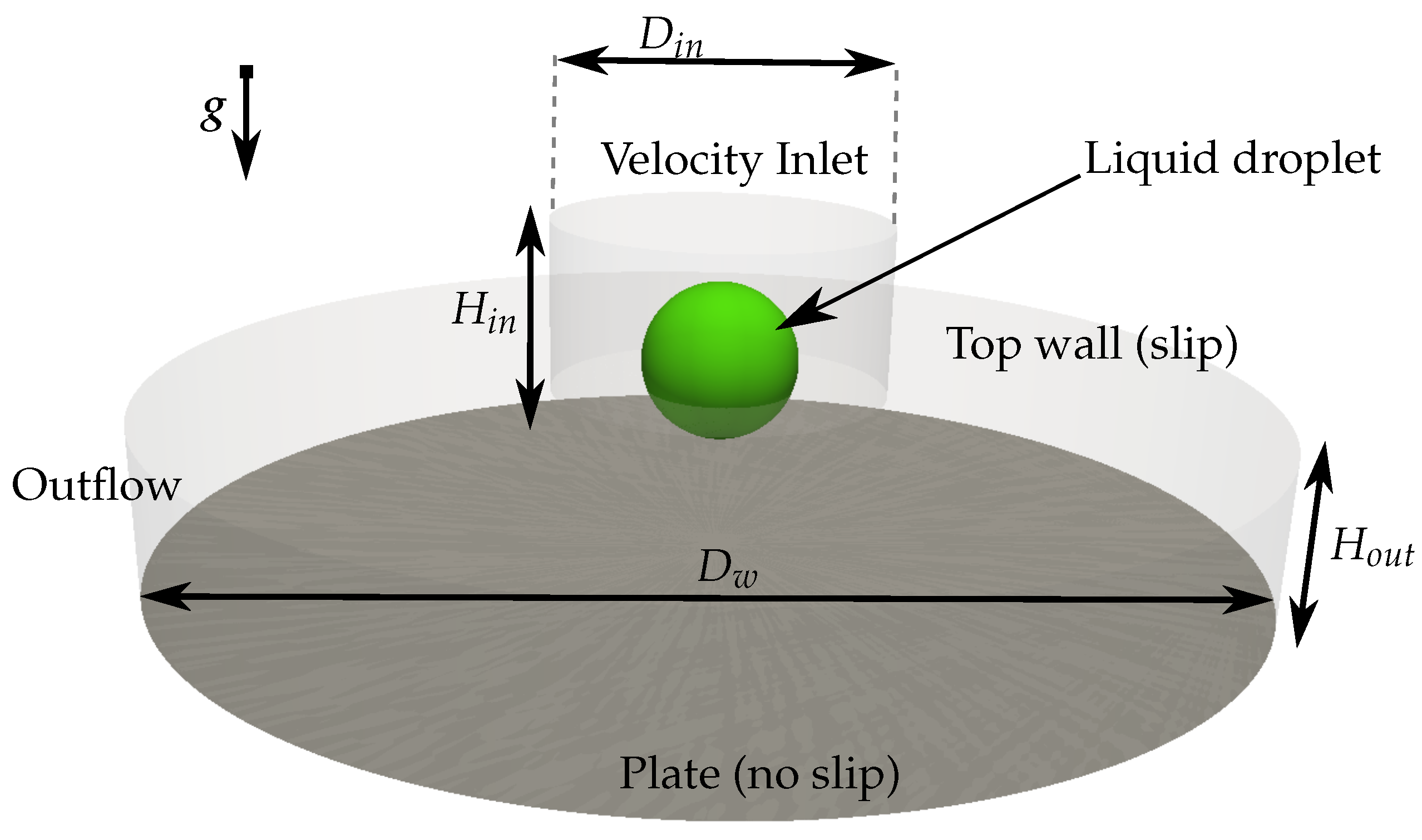
Figure 3.
Case 0 validation study with a qualitative comparison of experimental and simulated results. Upper row: experimental results from Rioboo [41] Lower row: Case 0 simulated results.
Figure 3.
Case 0 validation study with a qualitative comparison of experimental and simulated results. Upper row: experimental results from Rioboo [41] Lower row: Case 0 simulated results.
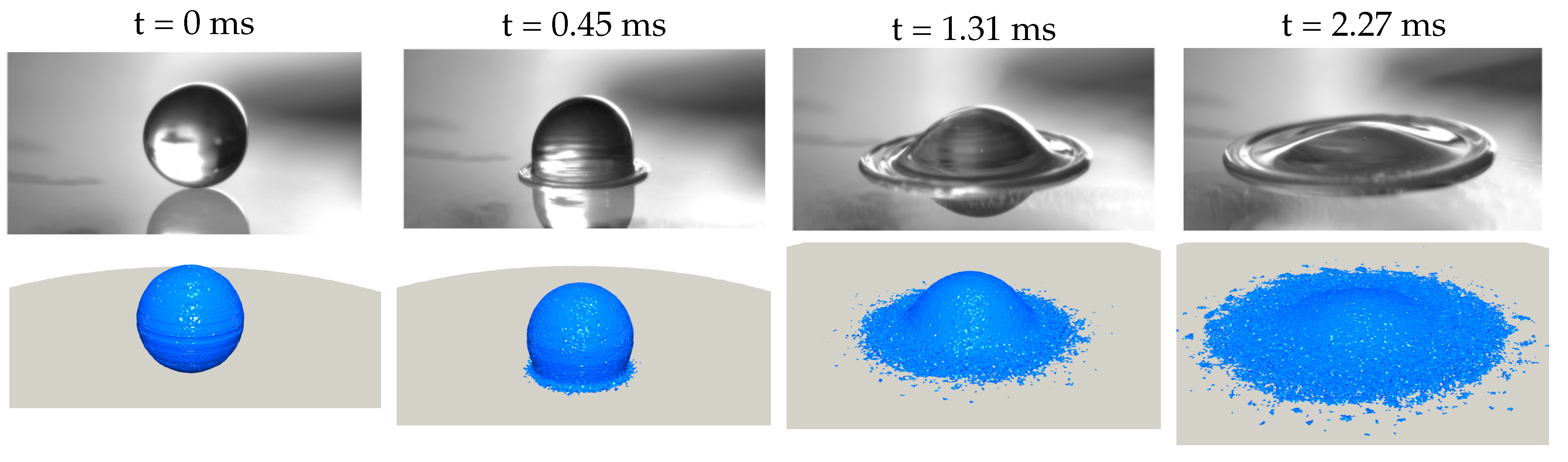
Figure 4.
Axisymmetric mean of the pressure for Case 0.
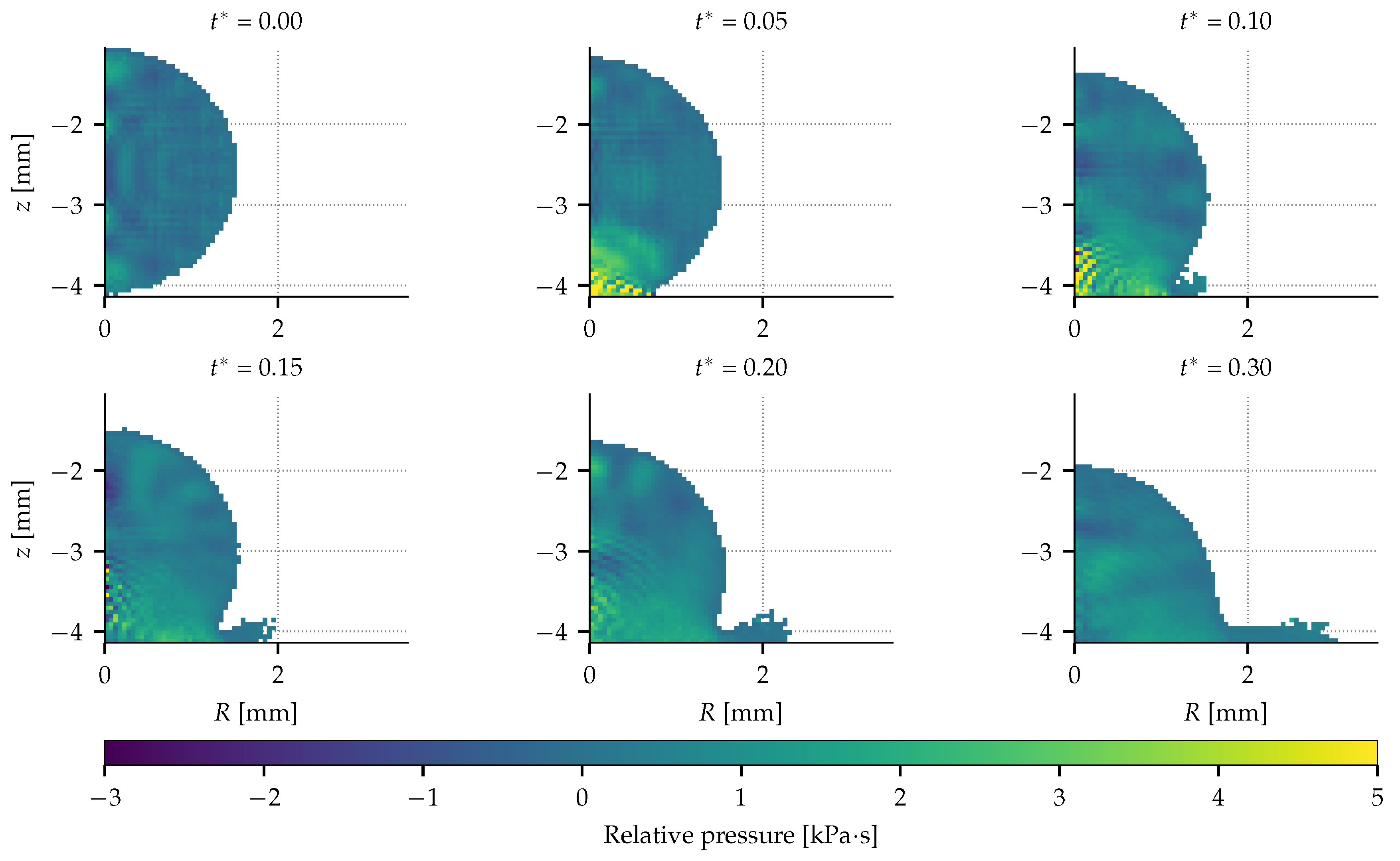
Figure 5.
Illustration of the methods to determine the liquid contact surface.
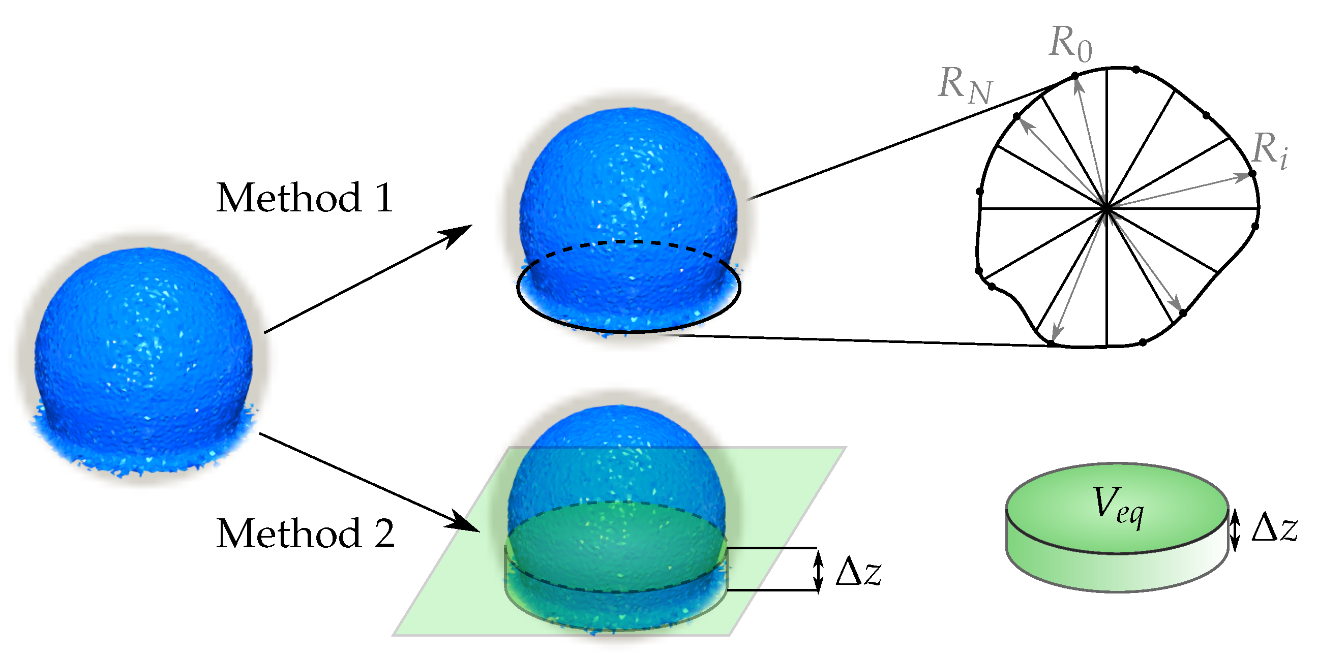
Figure 6.
Validation of the numerical model versus cases from [38]. Symbols represent the experiment while the plain and dashed lines represent Method 1 and Method 2, respectively.
Figure 6.
Validation of the numerical model versus cases from [38]. Symbols represent the experiment while the plain and dashed lines represent Method 1 and Method 2, respectively.
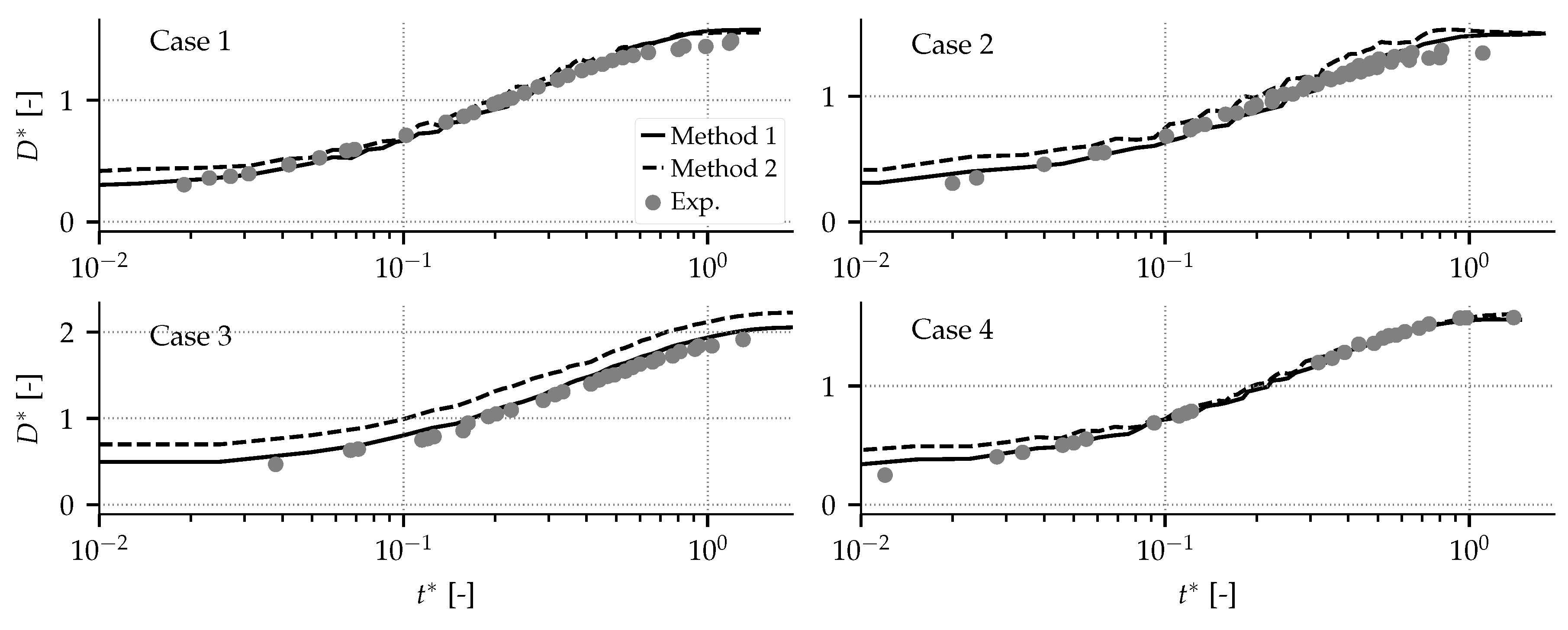
Figure 7.
Illustration of the particle deformation after impact. Particles are colored to reflect their z-coordinate (height above the surface of the wall) and those considered as having wall contact are marked in white.
Figure 7.
Illustration of the particle deformation after impact. Particles are colored to reflect their z-coordinate (height above the surface of the wall) and those considered as having wall contact are marked in white.

Figure 8.
Influence of the initial sand particle diameter (left) and normal velocity (right) on the impact transients in the nondimensional spreading diameter (top), total normal force (middle) and contact pressure (bottom) as a function of nondimensional time.
Figure 8.
Influence of the initial sand particle diameter (left) and normal velocity (right) on the impact transients in the nondimensional spreading diameter (top), total normal force (middle) and contact pressure (bottom) as a function of nondimensional time.
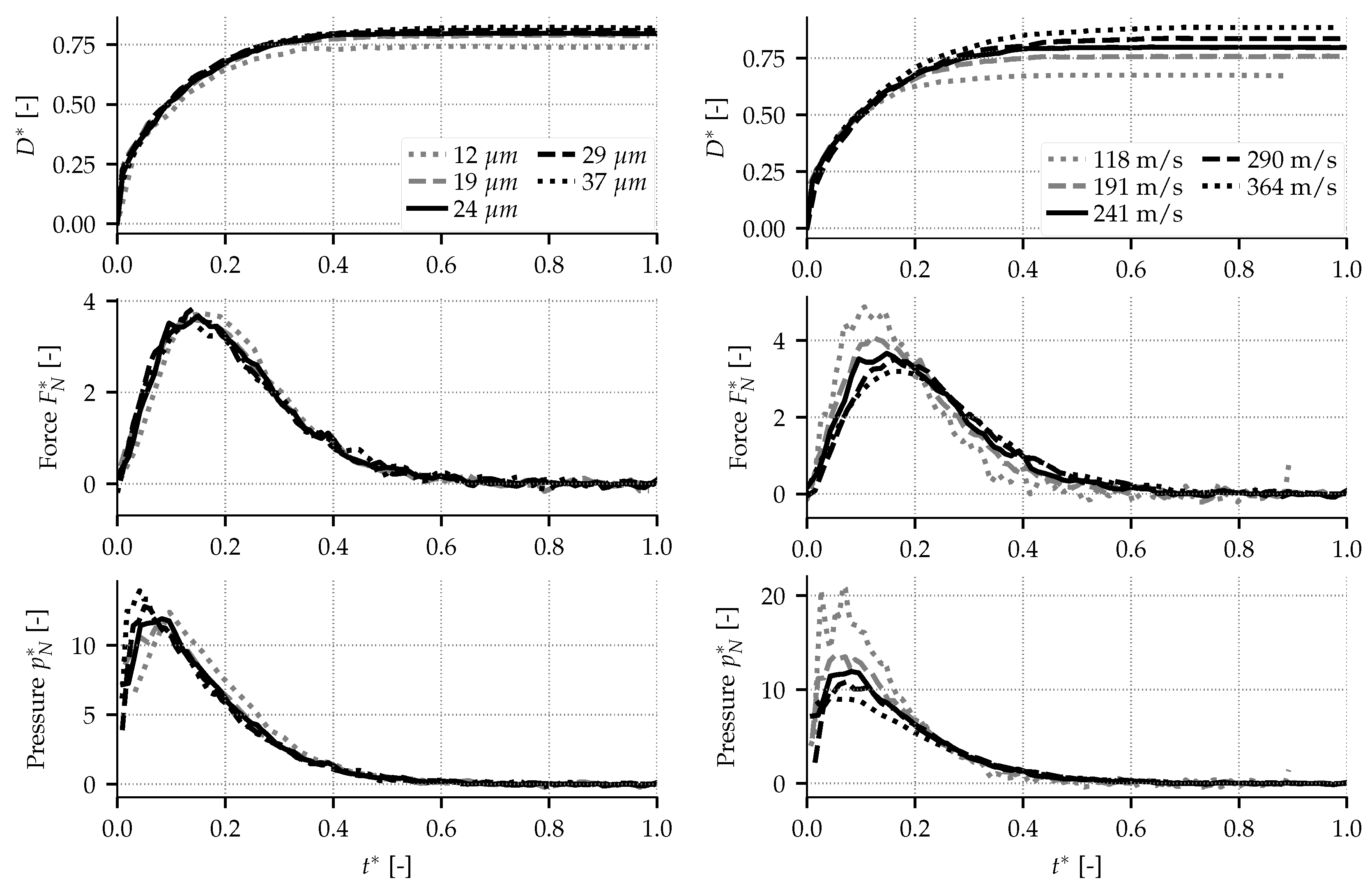
Figure 9.
Influence of the sand particle viscosity (left) and density (right) on the impact transients in the nondimensional spreading diameter (top), total normal force (middle) and contact pressure (bottom) as a function of nondimensional time.
Figure 9.
Influence of the sand particle viscosity (left) and density (right) on the impact transients in the nondimensional spreading diameter (top), total normal force (middle) and contact pressure (bottom) as a function of nondimensional time.

Figure 10.
Comparison of correlations from Table 4 with the values extracted from the numerical simulation.
Figure 10.
Comparison of correlations from Table 4 with the values extracted from the numerical simulation.
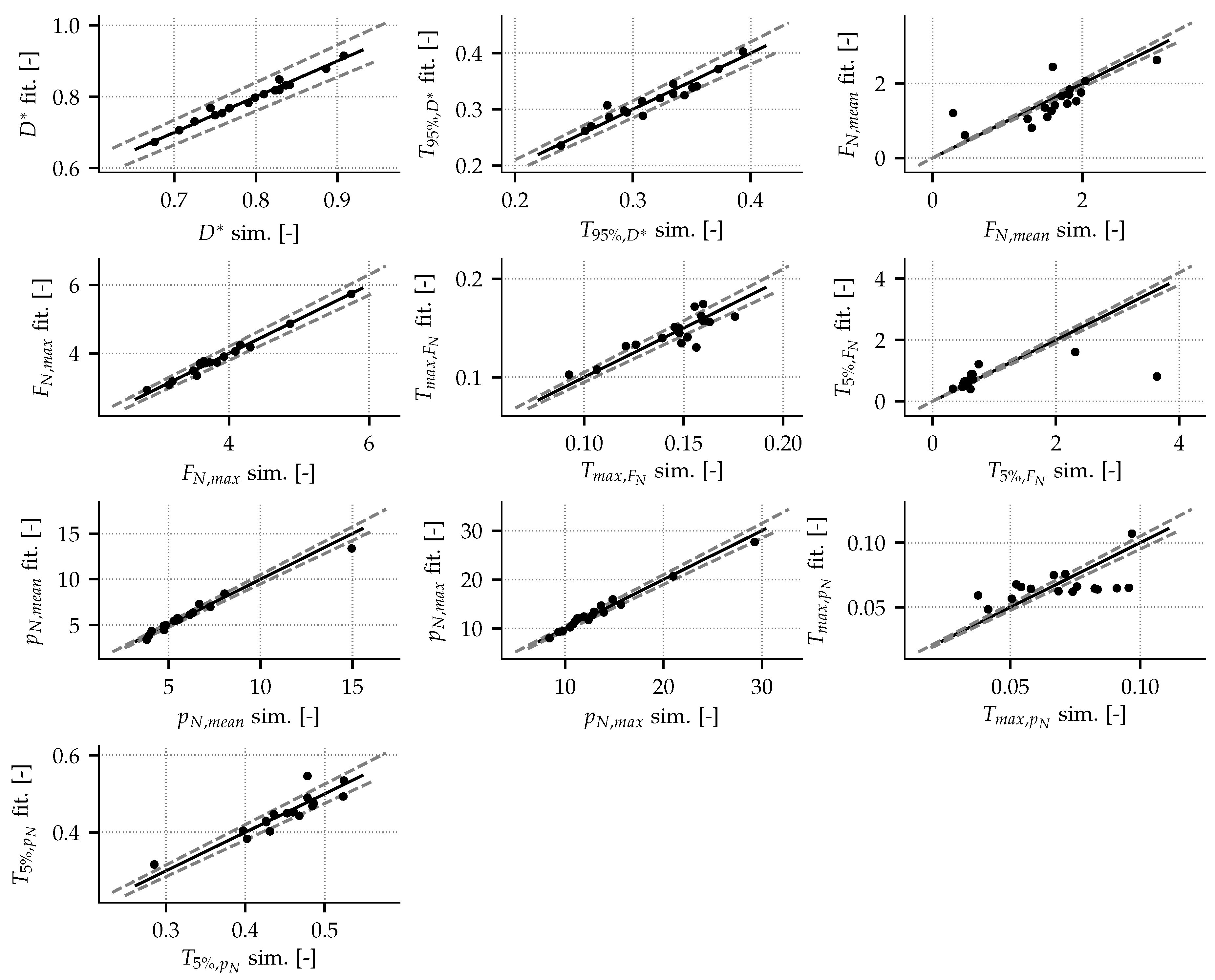
Figure 11.
Comparison of change in nondimensional spreading diameter (top), total normal force (middle) and contact pressure (bottom) with nondimensional time for the main cube orientations and the sphere (left) and for all cube impact orientations (right).
Figure 11.
Comparison of change in nondimensional spreading diameter (top), total normal force (middle) and contact pressure (bottom) with nondimensional time for the main cube orientations and the sphere (left) and for all cube impact orientations (right).
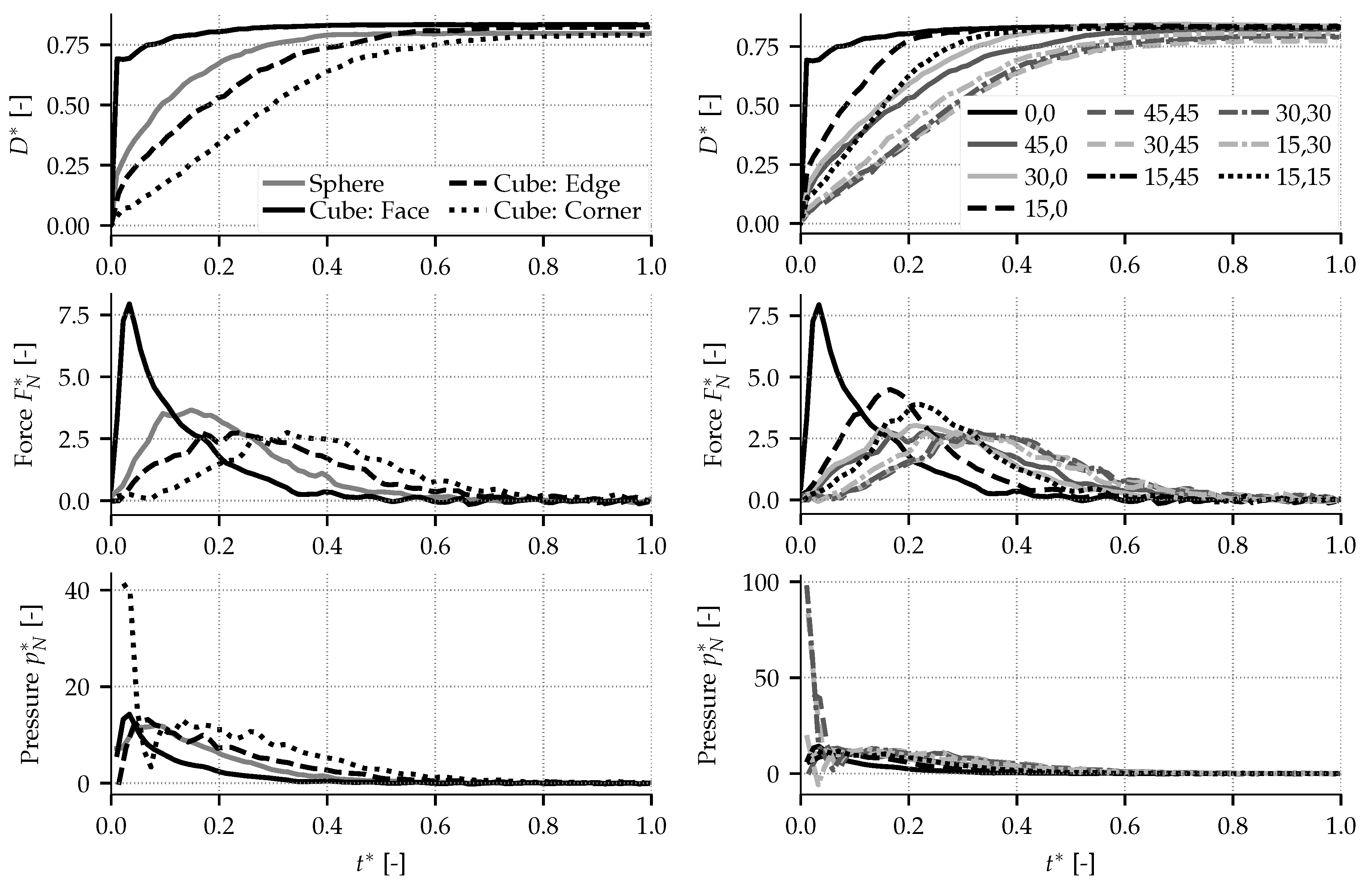
Figure 12.
Illustration of the impact of the cube presenting its face (a), edge perpendicular (b) and parallel (c) to the tangential velocity and its corner (d). The arrows represent the tangential velocity.
Figure 12.
Illustration of the impact of the cube presenting its face (a), edge perpendicular (b) and parallel (c) to the tangential velocity and its corner (d). The arrows represent the tangential velocity.
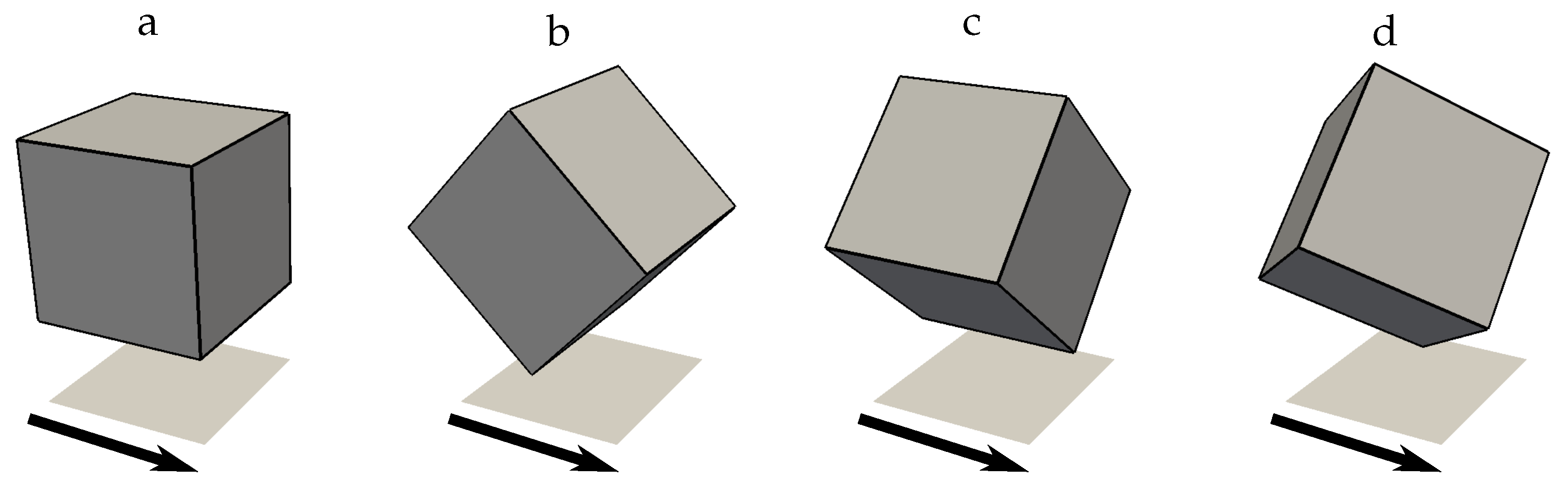
Figure 13.
Influence of the impact angle on the transients of a sphere.
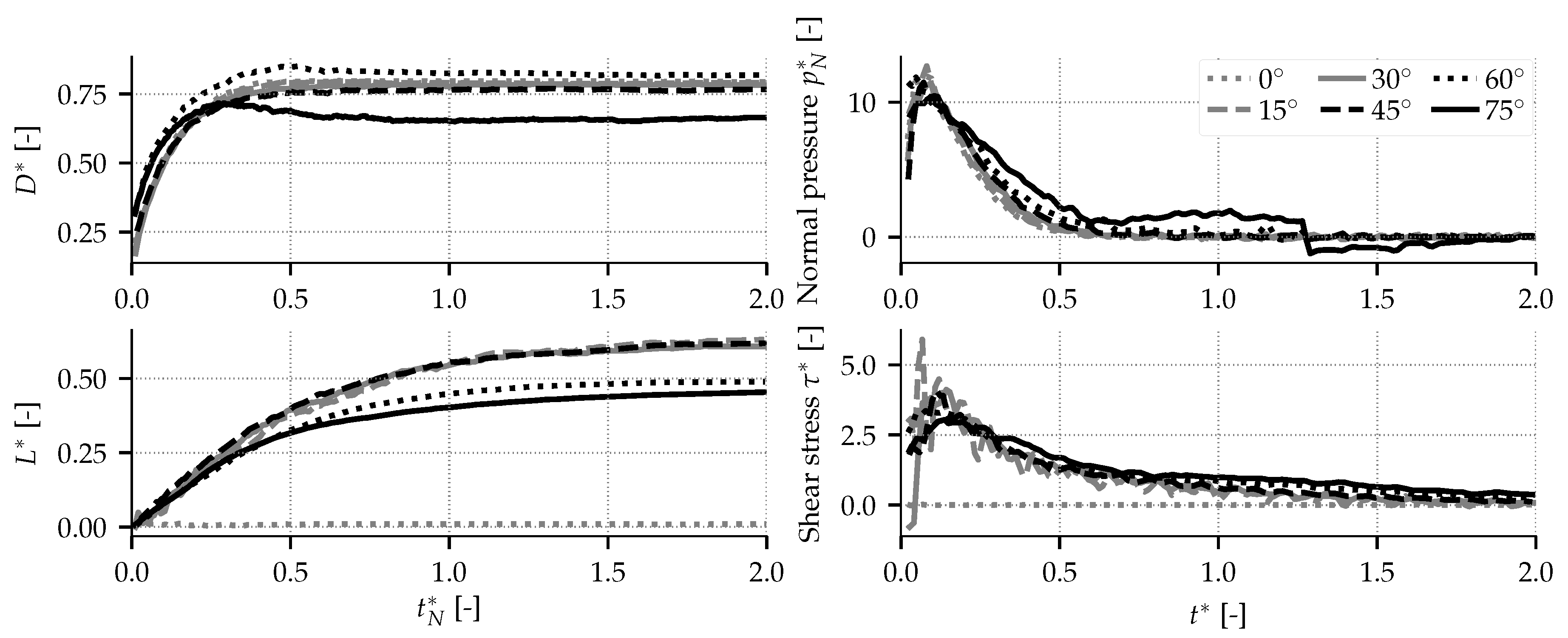
Figure 14.
Influence of the impact angle on the transient of a cube presenting its face.
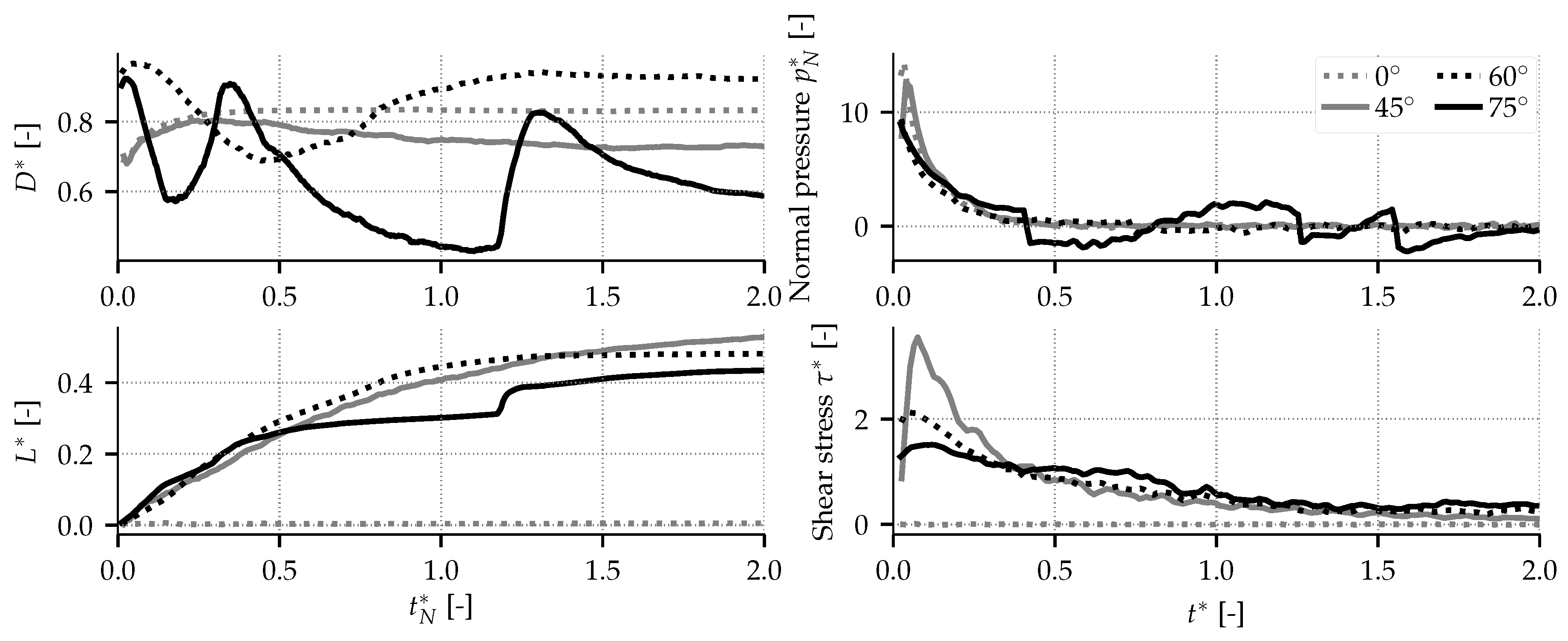
Figure 15.
Influence of the impact angle on the transient of a cube presenting its edge perpendicular to the tangential velocity component.
Figure 15.
Influence of the impact angle on the transient of a cube presenting its edge perpendicular to the tangential velocity component.
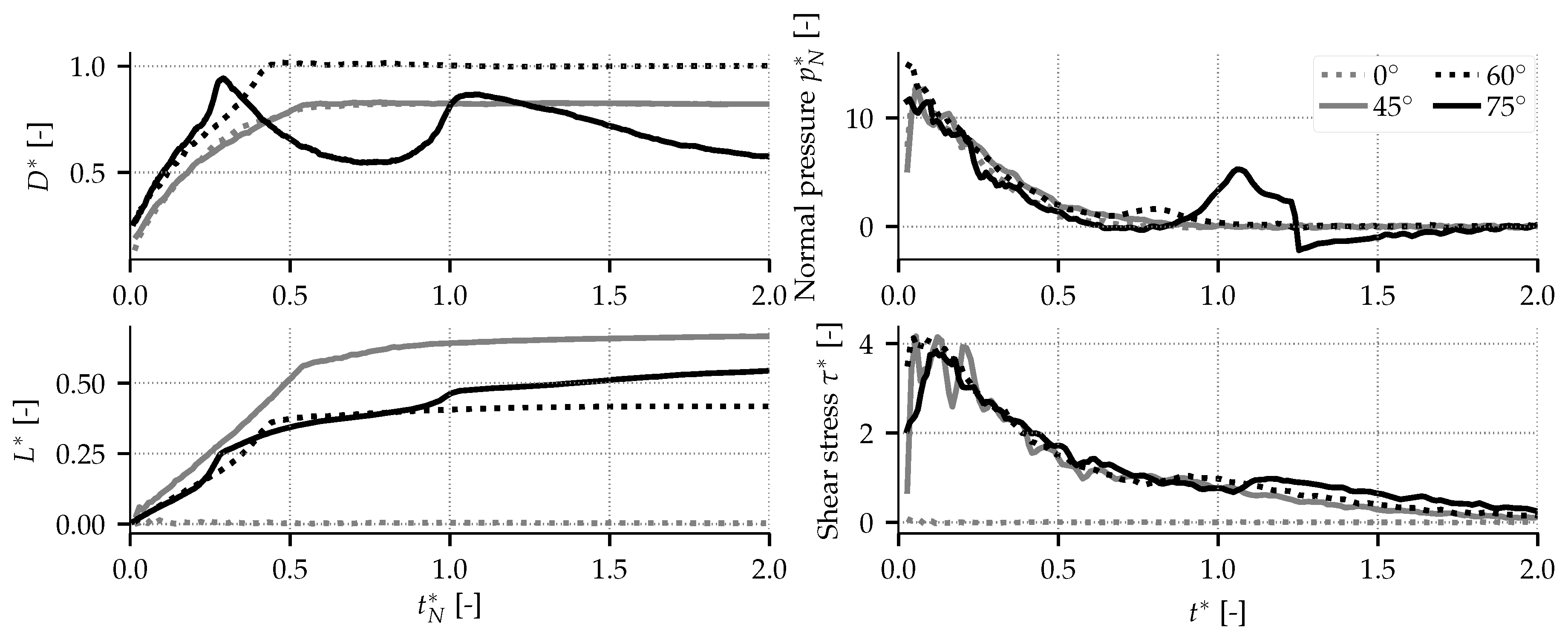
Figure 16.
Influence of the impact angle on the transient of a cube presenting its edge parallel to the tangential velocity component.
Figure 16.
Influence of the impact angle on the transient of a cube presenting its edge parallel to the tangential velocity component.
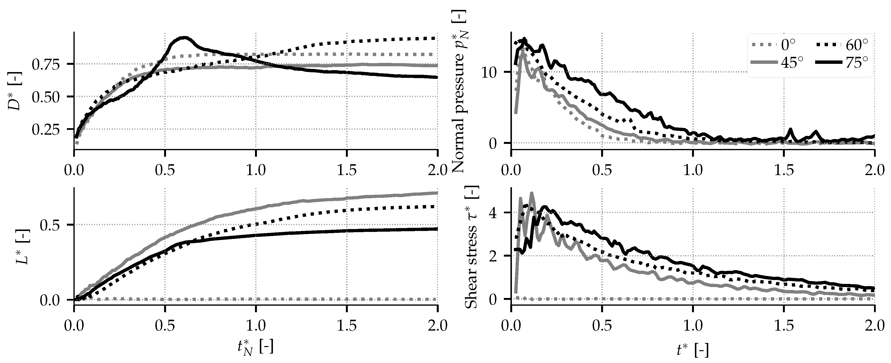
Figure 17.
Influence of the impact angle on the transient of a cube presenting its edge parallel to the tangential velocity component.
Figure 17.
Influence of the impact angle on the transient of a cube presenting its edge parallel to the tangential velocity component.
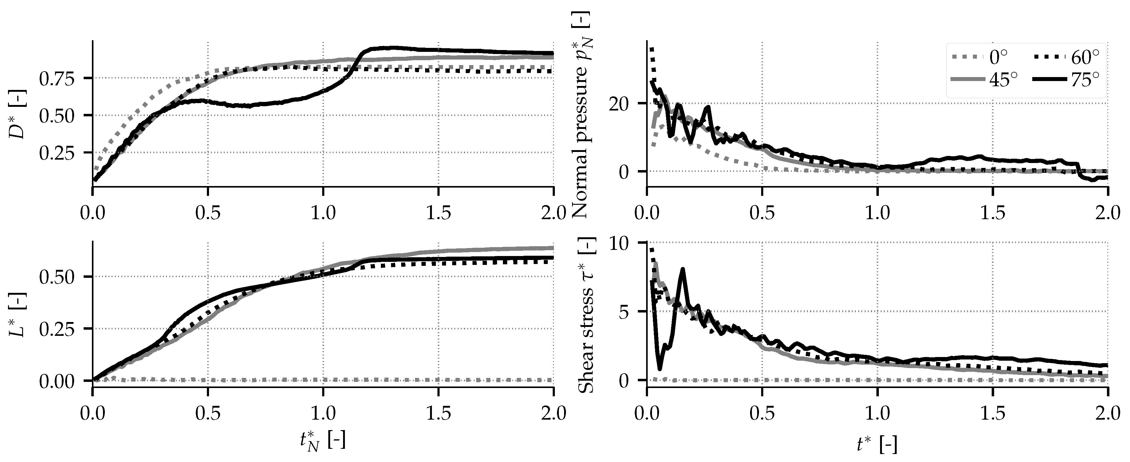
Figure 18.
Time series of the impact of the cube presenting its face (a), edge perpendicular (b) and parallel (c) to the tangential velocity and its corner (d) for an oblique impact of . Particles are colored by their unique identity tag.
Figure 18.
Time series of the impact of the cube presenting its face (a), edge perpendicular (b) and parallel (c) to the tangential velocity and its corner (d) for an oblique impact of . Particles are colored by their unique identity tag.

Table 1.
Dimensions of the numerical domains and the spatial discretization.
| Case | |||||
|---|---|---|---|---|---|
| - | [mm] | [mm] | [mm] | [mm] | [m] |
| Validation | 5 | 17 | 1.9 | 2 | 50 |
| Real conditions | 0.05 | 0.12 | 0.03 | 0.03 | 0.6 |
Table 2.
Operating parameters for validation, from [38].
Table 2.
Operating parameters for validation, from [38].
| Case | Liquid Type | Velocity | Diameter | Viscosity | Density | Surf. Tens. | Re | We | Oh |
|---|---|---|---|---|---|---|---|---|---|
| - | - | [m/s] | [mm] | [Pa·s] | [kg/m] | [kg/s] | [−] | [−] | [−] |
| 0 | Water | 1.18 | 3.04 | 0.001 | 1000 | 0.072 | 3587 | 59 | |
| 1 | Glycerin | 0.96 | 2.64 | 0.1 | 1260 | 0.063 | 32 | 49 | 0.22 |
| 2 | Glycerin | 2.70 | 2.65 | 0.1 | 1260 | 0.063 | 90 | 386 | 0.22 |
| 3 | Glycerin | 0.97 | 2.08 | 0.1 | 1260 | 0.063 | 25 | 39 | 0.25 |
| 4 | Silicone oil | 0.89 | 2.84 | 0.1 | 963 | 0.021 | 24 | 103 | 0.42 |
Table 3.
Operating parameters for the reference case.
| Velocity | Diameter | Viscosity | Density | Surf. Tens. | Re | We | Oh |
|---|---|---|---|---|---|---|---|
| [m/s] | [m] | [Pa·s] | [kg/m] | [kg/s] | [−] | [−] | [−] |
| 250 | 25 | 11 | 2665 | 0.4 | 1.83 | 12,600 | 61 |
Table 4.
Correlations on peak values. Variables a to e refer to those in Equation (18). Reference values are expressed in SI units in the formulae.
Table 4.
Correlations on peak values. Variables a to e refer to those in Equation (18). Reference values are expressed in SI units in the formulae.
| a | |||||
|---|---|---|---|---|---|
| Ref. Value | - | m/s | m | Pa·s | kg/m |
| 0.807 | 0.238 | 0.072 | −0.205 | 0.160 | |
| 0.319 | 0.407 | 0.094 | −0.366 | 0.240 | |
| 1.865 | −0.184 | 1.263 | 0.848 | −0.822 | |
| 3.745 | −0.379 | 0.022 | 0.278 | −0.596 | |
| 0.139 | 0.416 | −0.195 | −0.167 | 0.468 | |
| 0.520 | 0.169 | −1.284 | −0.864 | 0.691 | |
| 5.629 | −0.594 | 0.068 | 0.560 | −1.224 | |
| 12.833 | −0.715 | 0.137 | 0.416 | −1.098 | |
| 0.056 | −0.211 | −0.716 | 0.052 | −0.018 | |
| 0.447 | 0.225 | −0.027 | −0.254 | 0.486 |
© 2020 by the authors. Licensee MDPI, Basel, Switzerland. This article is an open access article distributed under the terms and conditions of the Creative Commons Attribution (CC BY) license (http://creativecommons.org/licenses/by/4.0/).
Share and Cite
MDPI and ACS Style
Chaussonnet, G.; Bravo, L.; Flatau, A.; Koch, R.; Bauer, H.-J. Smoothed Particle Hydrodynamics Simulation of High Velocity Impact Dynamics of Molten Sand Particles. Energies 2020, 13, 5134. https://doi.org/10.3390/en13195134
AMA Style
Chaussonnet G, Bravo L, Flatau A, Koch R, Bauer H-J. Smoothed Particle Hydrodynamics Simulation of High Velocity Impact Dynamics of Molten Sand Particles. Energies. 2020; 13(19):5134. https://doi.org/10.3390/en13195134
Chicago/Turabian StyleChaussonnet, Geoffroy, Luis Bravo, Alison Flatau, Rainer Koch, and Hans-Jörg Bauer. 2020. "Smoothed Particle Hydrodynamics Simulation of High Velocity Impact Dynamics of Molten Sand Particles" Energies 13, no. 19: 5134. https://doi.org/10.3390/en13195134
Note that from the first issue of 2016, this journal uses article numbers instead of page numbers. See further details here.