Dynamic Modeling of a Parallel-Connected Solid Oxide Fuel Cell Stack System


Department of Mechanical Engineering, National Chiao Tung University, Hsinchu 30010, Taiwan
*
Author to whom correspondence should be addressed.
Energies 2020, 13(2), 501; https://doi.org/10.3390/en13020501
Submission received: 20 November 2019
/
Revised: 18 January 2020
/
Accepted: 19 January 2020
/
Published: 20 January 2020
(This article belongs to the Section A5: Hydrogen Energy)
Abstract
:This study proposes novel simulation methods to model the power delivery function of a parallel-connected solid-oxide-fuel-cell stack system. The proposed methods are then used to investigate the possible thermal runaway induced by the performance mismatch between the employed stacks. A challenge in this modeling study is to achieve the same output voltage but different output current for each employed stack. Conventional fuel-cell models cannot be used, because they employ fuel flow rates and stack currents as the input variables. These two variables are unknown in the parallel-connected stack systems. The proposed method solves the aforementioned problems by integrating the fuel supply dynamics with the conventional stack models and then arranging them in a multiple-feedback-loop configuration for conducting simulations. The simulation results indicate that the proposed methods can model the transient response of the parallel-connected stack system. Moreover, for the dynamics of the power distribution, there exists an unstable positive feedback loop between employed stacks when the stack temperatures are low, and a stable negative feedback loop when the stack temperatures are high. A thermal runaway could be initiated when the dynamics of the stack temperature is slower than that of the current distribution.
1. Introduction
Fuel cells (FCs) have become a focus for power generation systems because of their environmentally friendly qualities and high energy-conversion efficiency [1,2]. An FC power plant has to aggregate several FC modules (approximately 10–50 kW), using power electronics such as DC-DC converters, to achieve the kilowatt or megawatt power capacity. Each FC module comprises several FC stacks (approximately 1–5 kW). Each stack contains several hundreds of cells, and each cell outputs a power of 20–30 W [3]. Because thousands of FC cells are within one FC module, each FC stack must have different characteristics due to manufacturing nonuniformity. Furthermore, inside each FC module, these FC stacks are often connected in parallel via mechanical manifolds for receiving the fuel supply and connected in parallel via electrical interconnection for obtaining the electricity output [4,5]. When connecting stacks with different characteristics in parallel, both the fuel supply and load distribution to each stack cannot be even. This nonuniformity problem can lead to severe stack operation and aging problems [6]. Therefore, currently, the uniformity requirement of the FC stack is strict, and the stack is expensive.
The stack resistance variation is one of the major concerns for the solid-oxide-fuel-cell (SOFC) system. The SOFC cell consists of porous electrodes with the thickness of tens of micrometers. Because of the fabrication technology, each cell is different from the other [7], such as electrode thickness and material uniformity. This also makes the initial resistance of each cell different [8]. Under SOFC operation conditions, the cell resistance would increase due to the electrode delamination, formation of hot spots, change in microstructures, etc. Consequently, the area-specific-resistance may increase from after of operations [9], which accounts for four times the resistance increase. For an FC stack comprising hundreds of cells, the stack resistance variation is enlarged because those cells are connected electrically in series and the contact resistance among them [10]. Besides, if one of the cells has a higher resistance than the others, it may exhibit a negative voltage across that cell. And, if this effect sets in, it would initiate a domino effect that accelerates the stack degradation [11,12]. Therefore, the stack resistance would not be the same in a multiple-stack system.
Thermal runaway is a phenomenon in which an increase in temperature changes operating conditions in a manner that causes a further rise in temperature and often leads to a destructive result. This phenomenon is frequently observed in exothermic chemical reactions and parallel-connected electronic components. For example, the hydrogen recombination process in a lithium-ion battery is exothermic. The elevated temperature would initiate a series of even stronger exothermic processes, which eventually burn the battery [13]. In electronics, thermal runaway is typically associated with increased current flow and power dissipation. This phenomenon can be initiated by the direct parallel operation of power devices when employed devices have different performance and the negative temperature coefficient of the on-state voltage [14].
Model simulation is one of the major approaches to investigate the behaviors of an FC system because it is costly to conduct the experiments with FC systems, especially for the high-temperature SOFCs. Various SOFC models have been proposed for different applications. The most popular ones are the static stack models that are often used for studying the operation points and the energy conversion efficiency of the FC systems [15,16]. Some researchers proposed dynamics stack models, which integrated the fuel supply dynamics with the static stack models, for developing the instrumentation strategies for the FC systems [17,18]. Most of the approaches above use the “lump model” to describe the stack behaviors, and they use stack current and fuel flow rates as the input variables [19,20]. Only a few researchers proposed “distributed models” to describe the stack behavior at different locations of the stack for better accuracy [21,22]. One challenge of constructing such a model is to comply with the following physics: the same voltage but different current at different locations. This constraint implies that the distributed model cannot be obtained by only stacking several “lumped models.” The distributed-model approaches solve this problem by incorporating numerical searches in the dynamics simulations [23,24]. To our best knowledge, we have not found an existing model for the parallel-connected stacks in a power module.
According to the aforementioned literature survey, a parallel-connected FC stack system contains several factors that could possibly initiate the thermal runaway such as negative temperature coefficient of the stack voltage, exothermic electrochemical reactions, nonuniform stack resistance, absence of power electronics for regulating power distribution, and nonuniformity of the fuel supply. However, we have not found any study that discusses the thermal runaway induced by the nonuniformity of the stack performance. In this study, we proposed the use of model simulations to investigate this issue. The employed model for this task should incorporate the modeling of the electrochemical reactions, fuel supply dynamics, electrical connections, temperature dynamics, etc. [25,26]. Conventional SOFC models cannot be applied because most of them use fuel flow rate and stack current as of the input variables. However, the values of these two variables depend on the other system dynamics in the parallel-connected fuel supply and parallel-connected electrical output systems. This study proposed a novel method to model the SOFC stacks in parallel. By using this model, we investigated the FC module behaviors when the employed FC stacks have different ohmic properties (stack resistance). The model construction, simulation methods, transient response of the SOFC module, and the possible cause of thermal runaway are discussed in detail in this paper.
2. Architecture of the Parallel-Connected FC Stacks
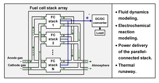
Figure 1 illustrates a schematic of the aggregated FC stacks that deliver electrical power to the load. Two FC stacks are used as an example without loss of generality. In this case, the inlet fuel (hydrogen and steam) is split into the anode channels of FC stack 1 and 2, and the inlet air (oxygen and nitrogen) is segregated into the cathode channels of FC stack 1 and 2. These gases pass through electrochemical reactions inside each FC stack, to generate electricity. The generated electricity is then connected in parallel to feed the DC–DC converter and to supply the external load. The outlets of the anode and cathode channels of each stack are merged to discharge the unused fuels and gases.
The power generation of the FC system depends on electrochemical reactions inside the FC stacks. These reactions are determined by factors such as the fluid mass flow rates, gas pressures, stack temperature, and power loading. The electrochemical reaction is complex because the aforementioned physics dynamics are all coupled together. Moreover, the reaction becomes more complicated when these stacks are connected in parallel. For example, the fuel distribution in a parallel-connected stack system varies with the channel pressures of each stack. Furthermore, the channel pressure and fuel composition in each stack are affected by electrochemical reactions, which are determined by the power distribution. However, the power distribution cannot be determined without knowing the operation conditions of each stack first. The aforementioned statements indicate that those physic dynamics are not only coupled inside FC stacks but also across FC stacks.
The DC–DC converter is used to isolate the power module from the external load and to maintain a stable voltage at the load. Moreover, the converter prevents the current from flowing back into power modules when power modules with different characteristics are connected together. A conventional DC–DC converter mainly comprises a pulse width modulation (PWM) regulator, capacitor, inductor, switch, diode, and resistor. In this configuration, when the power module does not supply sufficient power to the load, the load voltage is less than its designated value. The feedback signal requests the PWM regulator to increase the duty ratio of the switch control signal, and thus the inductor drains more current out of the power module. In other words, when adapting the DC–DC converter, the power request from the load is converted to the output current request of the power module.
3. Mathematics Models of the Parallel-Connected SOFC Stacks
According to the system configuration displayed in Figure 1, the system model should include the dynamics of the electrochemical reactions, thermal fluid, and power electronics (such as DC–DC converter). However, because the dynamics of the DC–DC converter is much faster than the others, the dynamics of the DC–DC converter is neglected in the simulations for simplicity.
3.1. Fluid Dynamics Modeling
The mass of each gas inside the FC stack can be modeled by the law of conservation of mass. By using the anode channel as an example, the mass of gas in the FC stack is described as follows:
where , , and are the inlet, reactive, and outlet mass flow rates of gas , respectively; represents the number of cells in an FC stack; is the current output of the stack , , and are the mole fractions of gas of the stack ; denotes the fuel entering rate; and represents the discharging rate. According to [27], the mass flow rate can be modeled by linearizing the flow equation of the nozzle when the pressure difference between upstream and downstream is small and the flow is operating in the subcritical region. Therefore, and can be modeled as follows:
where and are the two constants of the inlet and outlet flow rates; and are the upstream and downstream pressures of the stack; and is the anode channel pressure of the stack . Because the inlets (outlets) of the two stacks are connected, the inlet and outlet pressures of the two stacks are the same. Similarly, the mass of the gases in the cathode channel ( and ) can be calculated analogously by using Equations (1)–(6).
The gas pressure in the anode channel can be modeled by using the ideal gas law as follows [20]:
where is the gas constant, is the volume of the anode channel, and represents the stack temperature. The FC stack temperature can be modeled by using the energy conservation law as follows:
where is the effective area of the heat radiation, is the emissivity of air, and denotes the Boltzman constant [28]. Here, and are the equivalent mass and specific heat capacity of the FC cell, respectively. Moreover, and are the equivalent mass and specific heat capacity of the interconnector, respectively, and and are the equivalent mass and specific heat capacity of the stack fixture. is the electricity power of the FC stack, and and represent the temperatures of the gases entering the anode channel and the cathode channel, respectively. is the specific heat capacity of gas, ; is the reaction heat of the electrochemical reactions; and is the thermal radiation between stacks.
3.2. Electrochemical Reaction Modeling
In an SOFC stack, oxygen dissociates into oxygen ions when it receives electrons from cathode electrodes. The oxygen ions pass through the electrolyte and react with hydrogen in the anode channel. These reactions generate electrons to source the external load. The ideal cell voltage in the stack can be described by using the Nernst equation [19,20].
where represents the Gibbs free energy, is the ideal gas constant, and is the Faraday constant. Several voltage loss (polarization) mechanisms are present when the FC cell is delivering currents. The output voltage of the FC cell is modeled as follows:
where is the activation polarization, is the ohmic polarization, represents the concentration polarization, is the output current density of a cell, and is the ohmic deterioration factor. , , , , , and are the ohmic-loss coefficients of the electrodes; , , and are the thicknesses of the electrodes; and represent the respective exchange current density of the anode and cathode for calculating the activation polarization; and and are the respective limiting current densities of the anode and cathode for calculating the concentration polarizations. The aforementioned current density can be obtained by the following equation [29,30]:
where , , , and are the activation polarization coefficients, and and represents the effective gaseous diffusivities through the electrode. According to Equations (13)–(21), the cell voltage depends on the gas pressure, output current, and stack temperature. Moreover, both the Nernst voltage and ohmic polarization have negative temperature coefficients. Both the concentration and activation polarizations are complicated functions of the stack temperature.
Equations (1)–(12) can be used to obtain the gas mass, gas pressure, and stack temperature. The values of these parameters are fed into Equations (13)–(21), to calculate the output voltage of a single cell. Finally, the output current (), stack voltage (), and output power () of the stack can be calculated as follows:
where is the cell area. The stack model displayed above is very similar to the lumped stack model used in previous studies [19,20]. It differs from the lumped stack model in the following aspects: (1) a flow rate model is included to distribute the fuel to each stack, and (2) the heat radiation term, , should be included to model the heat exchange between stacks. Note that Equations (13)–(21) indicate that the stack voltage can be calculated when the stack current and chamber pressure are specified beforehand.
4. Proposed Algorithms for Modeling the Parallel-Connected Stacks
To comply with physics specifications, each power module in a parallel-connected network should have the same output voltage. Moreover, when power electronics are adapted to connect the power modules and the load, the output characteristics (current and voltage) of the power module are uncertain. The aforementioned statements are particularly true for an FC system because the system is not a constant-voltage source. Thus, conventional stack models that use the stack current as input variables to determine the stack voltage must be applied in different manners to model the parallel-connected FC stack system.
Figure 2 presents a block diagram of the proposed simulation method that can model the power-delivering function of the FC system displayed in Figure 1. The proposed method arranges two FC stack models in a multiple-feedback-loop system. Each stack model comprises the expressions presented in Equations (13)–(21), which use the stack current as the input to determine the stack voltage and the output power. Each stack voltage and output power values are used to calculate the averaged stack voltage and total power output of the multiple-stack system. Because the response from the power input to the voltage output of the DC–DC converter is much faster than that of the electrochemical reactions, the DC–DC converter is modeled as an energy-conversion factor (), as shown in Figure 2.
In a parallel-connected power system, the output current of each module should adhere to two requirements: (1) the current distribution should ensure that the voltage output of each module is the same, and (2) the total output power should be sufficient to maintain the designated load voltage. These two requirements are ensured by two sets of feedback loops that are shown in Figure 2. The first set of loops feedback each stack voltage and the averaged stack voltage. The difference between these two voltages is processed by the integral operations to determine a portion of the stack current ( and , noted in the plot). The second set of loops feedback the total power delivered. The difference between the delivered power and the designated load power (Pref, in Figure 2) is also processed by using the integral operations to determine another portion of the stack current (, in Figure 2). If the parameters of these three integral operations (KI1, KI2, and KI3) are designed properly, the two stack voltages should be the same. Moreover, the power delivery would be the same as the designated load power.
Parameter Design for Integral Operations
The design of the parameters must satisfy the following constraints: (1) every feedback loop of the system shown in Figure 2 should be stable, (2) the outcome of the current distribution should not be influenced by the part of the algorithms in which the same voltage is achieved for the two stacks, and (3) the model displayed in Figure 2 should present the dynamics of the power-delivering function of the FC system. According to the block diagram presented in Figure 2, the total output current of the system is as follows:
To ensure that the current distribution is not disturbed by the history of the searching process, and . Moreover, must be designed in a manner such that all the feedback loops are stable and the convergence of is fast. Therefore, (, 2) could represent the transient response of the stack voltage and current of the parallel-connected system. In this manner, the output power of the system can be described as follows.
After taking the Laplace transformation of the aforementioned equation, the dynamics of the power-delivering function can be approximated as follows:
where is the stack voltage at the operation point. According to Equation (27), the value of is determined by the response time of the FC system. Moreover, the values of should be set based on the stability and bandwidth of the feedback system displayed in Figure 2. However, the FC system is highly nonlinear, and the stability analysis of the system is not the focus of this study. We designed the values of by using empirical methods. Moreover, a suitable selection of the values of these parameters is as follows: and .
5. Simulation Results
In this study, we used the MATLAB/Simulink (MathWorks, Massachusetts, United States) to construct the model and investigate the performance of the FC system. We first validated the proposed models and simulation methods and then checked the performance of the system when the employed stacks have different characteristics. The parameters of the SOFC stack model are listed in Table 1 and Table 2. Table 1 lists the parameters of the thermal-fluid dynamics of the stack. All of these parameters, except for the mass of the stack fixture, are excerpted from a previous study [30]. Table 2 lists the parameters of electrochemical reactions. All of these parameters, except for the cell area, , and the number of cells in a stack, , are excerpted from a study [30].
5.1. Model Validation
Ideally, the proposed model and simulation methods should be verified by using the experimental results of the stack transient response. Unfortunately, we could not find those data in the literature. Instead, we compared our results with the experimental results of the static stack response presented in [31] for different operating temperatures, as shown in Figure 3. The static stack response (I–V curve) was tested under the following conditions: 97% of hydrogen and 3% of steam in the anode channel, 21% of oxygen and 79% of nitrogen in the cathode channel, 101325 Pa of the anode and cathode pressures, and stack temperature ranging from 873 to 1073 K. Experimental results excerpted from the aforementioned study [31] were denoted by solid-marks (triangles, circles, and diamonds); the I–V curve predicted by the static stack model (Equations (13)–(21) and parameters listed in Table 2) was represented by hollow-marks, and predicted by the steady-state value of the dynamic models (Equations (1)–(21) and parameters listed in Table 1 and Table 2) were depicted by a red line. According to the plot, the proposed model predicts less polarization loss than the experimental data. The averaged relative-error between the static model and experimental data is 11.6%. Besides, the results from the proposed dynamic model are very close to the static stack model at the temperature of 873 K.
5.2. Dynamic Response of the Parallel-Connected SOFC Stacks
In the following simulations, the initial temperature of the two FC stacks was . Moreover, the initial pressures were and for the anode and cathode channels, respectively. From to s, the load power requirement ramped up from 0 to at a rate of . From to s, the load power was maintained at 1500 W. For comparison purposes, the next few figures reveal the performance of each stack under two operating conditions. The responses of stack 1 in case 1, stack 2 in case 1, stack 1 in case 2, and stack 2 in case 2 were represented by blue line, green dotted line, red dotted line, and purple dashed line, respectively.
5.2.1. Same Stacks in the Parallel Connection
In this simulation, stacks with the same performance were connected in parallel for the power delivery. The ohmic deterioration factors, presented in Equation (16), of the two stacks were () = (1, 1) in case 1 and () = (3.5, 3.5) in case 2. Figure 4 displays the dynamic response of the output current, voltage, output power, and temperature of each stack. According to the simulation results, both stacks had the same response because they were exactly the same. At the end of the simulation time, both stacks exhibited responses of , , and in case 1 and , , and in case 2. Both systems output power of 1500 W, as required. The dynamics of the stack temperature was slower than that of power delivery. Moreover, an FC system employing small ohmic-loss stacks delivered smaller currents, provided higher voltages, and had a lower stack temperature compared with a system employing large ohmic-loss stacks.
Figure 5 displays the response of the stack voltage composition, which includes Nernst voltage, activation polarization, ohmic polarization, and concentration polarization. According to simulation results, the Nernst voltage decreased as time increased, because of its negative temperature coefficient. Both activation and ohmic polarizations increased rapidly at the beginning and then decreased slowly. This phenomenon occurs because the output current increased rapidly at the beginning, and then the stack temperature increased slowly and dominated the response. The concentration polarization increased at the beginning, due to the increase in the output current, and kept increasing due to its positive temperature coefficient.
Figure 6 presents the anode channel pressure, cathode channel pressure, hydrogen utilization, and oxygen utilization in this example. According to simulation results, the anode and cathode pressures were and , respectively, in both cases. The hydrogen utilization was 61.4% in case 1 and 66.2% in case 2, whereas the oxygen utilization was 47.7% in case 1 and 51.1% in case 2. These simulation results indicated that the channel pressure did not vary significantly when the current (electrochemical reactions) in two cases varied from 67.6 to 62.7 A.
5.2.2. Different Stacks in the Parallel Connection
In this simulation, stacks that have different ohmic properties were connected in parallel for the power delivery function. The ohmic deterioration factors of the two stacks were () = (1, 3.5) in both cases. Case 1 includes the heat exchange between two stacks , and case 2 excluded . Figure 7 shows the dynamic response of the stack current, voltage, power, and temperature of each stack. In case 1, the output current of stack 1 (small ohmic loss) was much larger than that of stack 2 (large ohmic loss) during the power ramp up. The current of stack 2 slowly became equivalent to stack 1 as time increased. At s, the currents of stacks 1 and 2 were 67 and 63.2 A, which correspond to the power output of 771.9 and 728.1 W, respectively. Both stacks had the same voltage even when they had different currents. The temperature responses of the two stacks were almost the same due to the heat radiation. In case 2, stack 1 still retained a larger current output than stack 2. Both currents increased and the simulation terminated when the current of stack 1 attained a value of 98.4 A, which was the current limit ( in Equation (20)) of the concentration polarization. The temperature responses of the two stacks differed largely from each other because there was no heat exchange between them. According to these simulation results, the parallel-connected stacks that had different ohmic properties encountered a thermal runaway when the heat exchange between stacks was prohibited. Moreover, compared with the temperature results presented in the previous simulation, the output current in this case attained its current limit, which was not resulted from the stack temperature. This suggests that the temperature control of the power module may not be useful to prevent this thermal runaway from occurring.
Figure 8 displays the response of the stack voltage compositions in this example. In case 1, the stack voltage compositions were slightly different from those presented in Section 5.2.1, due to the different current distributions. In case 2, the Nernst voltages of the two stacks differed largely due to the large temperature difference between the two stacks. Moreover, the concentration polarization increased sharply because the output current reached its maximum current limit. This led to the zero stack voltage shown in Figure 7.
Figure 9 displays the channel pressure and fuel utilization in this example. According to the simulation results, in both cases, the anode channel pressures of the two stacks were stable at , while the cathode channel pressures varied from to . The pressure variation was less than 0.8% when the current output varied from 0 to 98.4 A. In case 1, the hydrogen utilization rates of the two stacks were 65.6% and 61.6%, and the oxygen utilization rates were 50.7% and 48.0%. In case 2, the hydrogen utilization rates of stack 1 reached 100%. Therefore, it can be concluded that the channel pressure and, thus, the inlet fuel distribution are not the major reasons that caused the instability.
5.2.3. Stacks Have Less Heat Capacity
In this simulation, the stack parameters were the same as those used in Section 5.2.2, except that the equivalent fixture masses ( in Equation (8)) of the two stacks were reduced to 0.01 mste. According to the results presented in Figure 10, in case 1 (allows heat exchange between stacks), stack 1 had an output of . According to the results presented in Figure 10, in case 1 (allows heat exchange between stacks), stack 1 had an output of 63.5 A, , , and , and stack 2 had an output of , , , and . The stack with the small ohmic loss had a larger output power than the stack with a large ohmic loss. In case 2 (without heat exchange between stacks), the transient responses of stacks were similar to those in case 1. However, the performance difference between stacks in case 2 was larger than that in case 1. Moreover, stack 2 had almost the same steady-state performance as that in stack 1, although the employed stacks are different, and no heat was exchanged between them.
6. Discussion
This study proposed a novel method to model the current distribution of parallel-connected SOFC stacks. According to the simulation results presented in Figure 4, Figure 7, and Figure 10, each parallel-connected stack has the same stack voltage, even when its output current differs from the others or is unbounded in some cases. Therefore, the proposed method is effective to solve this “same voltage but different current” problem. Moreover, the proposed method is better than the existing approaches that employ numerical searches to find the current distribution due to its lower amount of effort on the algorithm implementation. For example, a 50 kW SOFC power module normally comprises eight stacks in parallel [4]. To find the current distribution by conducting a numerical search, one has to derive an 8 × 8 Jacobian matrix for those highly nonlinear dynamics presented in Equations (13)–(21) and may also have to perform the matrix inversion. By contrast, the proposed method only requires eight feedback loops, which largely reduce the simulation effort required.
As aforementioned, the power-delivering behavior of the parallel-connected FC stacks is complicated because of the coupled physics inside the stacks and across stacks. Those coupled physics can be classified as fluid, electric, and thermal dynamics. According to the simulation results illustrated in Figure 5 and Figure 8, the channel pressures varied by less than 0.8% when the output current varied from 0 to 98.4 A. The channel pressures do not vary much, because the same amount of steam is generated when the hydrogen is consumed in the anode channel. Moreover, oxygen only accounts for approximately 10% of the total volume in the cathode channel. After excluding the effect of channel pressure (fluid dynamics), the power distribution is dominated by the coupled dynamics between electricity and temperature.
Case 1 in Section 5.2.2 presents the system response when the parallel-connected stacks have different ohmic properties. Because the two stack temperatures are almost the same (Figure 4d), the temperature effect can be excluded from the power (current) distribution. Moreover, if we only focus on the current difference in the two stacks, the portion of the current that is responsible for the load power delivery ( in Figure 2) can be ignored. Consequently, the current distribution is determined by the current that makes the two stack voltages the same ( and in Figure 2). In that case, is larger than at the beginning because stack 1 has a smaller ohmic loss than stack 2. Due to the increase in the power demand, increases. Thus, the difference between and has to be increased to compensate for the enlarged difference of the ohmic polarization. The stack temperature increases with the stack currents and then dominates all the polarization losses. Thus, the polarization differences between stacks and current distribution decreases. These mechanisms explain why the current is almost equally distributed in the steady state, albeit the employed stacks have different ohmic properties.
When the temperature effect is included, the power-sharing function in the parallel-connected system is very complicated. Figure 11 shows the plot of the cell voltage versus temperature by using Equations (13)–(21), when the pressure effect is excluded from the calculations. According to the plot, the stack voltage decreases as the stack current increases. Moreover, the stack voltages have positive temperature coefficients in the low-temperature and large-current region. The lower the temperature and the larger the current are, the more positive the temperature coefficients are. When the stack temperature increases, the stack voltages are less affected by the current, and their temperature coefficients decrease gradually and become negative.
Because the electrochemical reaction is exothermic, the stack that outputs a higher amount of current would have a higher stack temperature. In the parallel-connected stack system, the stacks that have the more positive temperature coefficients have to output a higher amount of current than the others to establish the same stack voltage. In the example presented in case 2 in Section 5.2.2, the initial current of stack 1 is larger than that of stack 2 due to the smaller ohmic loss of stack 1. The temperature coefficient of the stack 1 (large current) is more positive than that of stack 2 (small current) when both stack temperatures are low. Consequently, these two parallel-connected stacks enter a positive feedback loop, and the current difference between stacks increases sharply. Simultaneously, both stack currents increase due to the load demand. Before the temperatures of both stacks increase, which would minimize the polarization difference between stacks, the current of stack 1 attains its maximum current limit. These mechanisms explain the thermal runaway induced by the mismatch between the stack characteristics. In case 2, presented in Section 5.2.3, the temperature response is rapid. The increase in the temperature of stack 1 decreases the temperature coefficient of its stack voltage. Thus, the value of the coefficient is close to that of stack 2. The unstable current distribution may either exist only for a short duration or may not exist at all. Since both stack currents increase stably, the stack temperatures increase and the polarization differences between stacks decrease. Consequently, both the stack currents and stack temperatures are similar to each other, albeit there is no heat exchange between stacks.
According to the aforementioned analysis, the mismatches of the temperature coefficients and stack currents establish an unstable positive feedback loop across the stacks in the low-temperature region. Moreover, there is a stable negative feedback loop for minimizing the performance difference of the employed stacks when the stack temperature is high. Due to the interactions between the two aforementioned feedback loops, thermal runaway may occur in the following cases: (1) a large power requirement leads to a large-current output and higher stack temperatures, which in turns lower the maximum current limit, and (2) slow temperature dynamics compares to the current distribution dynamics, which enlarges the current differences between stacks. Thus, one of the employed stacks attain its maximum current limit.
According to the system configuration shown in Figure 1, load power shortage always leads to an increase in the stack current. This is because of the associated power electronics and the associated control methods presented in Figure 1. However, increase in the power output of the FC systems can be realized by either increasing or decreasing the output current, depending on the operation point. The proposed analysis suggests that it is beneficial to develop power electronics exclusively for FC systems. Thus, the employed FC stacks may have larger performance differences and the parallel-connected system can operate closer to its maximum power operation point. Further study of this problem will be conducted in the future.
7. Conclusions
This study proposed a novel method to model the power delivering operation of a parallel-connected SOFC system. This model comprises a parallel-connected fuel supply architecture, parallel-connected electrical output, and heat transfer between stacks. One of the challenges in this task is to obtain the same voltage but different current output for each employed stack. The proposed method solves this problem by using multiple feedback loops with the integral actions in the computation algorithms. The simulation results of this study indicated that when the proposed methods are used, the parallel-connected stacks have the same voltage output when each stack current is different or unbounded.
The proposed model and simulation methods were then used to investigate the possible thermal runaway induced by the mismatch between the stack performance. In these simulations, the required load power ramped up from 0 to 1500 W, at a rate of . The simulation results indicate that, when the two stacks are the same, even they have degenerated (the ohmic polarization increases 3.5 times), the parallel-connected stack system can deliver the power that is requested. However, when the employed stacks are different (one stack’s ohmic polarization is 3.5 times higher than that of the other), the parallel-connected stack system may become unstable when the temperature response is slow and the heat transfer between stacks is insufficient.
This study indicates that the mismatches between the temperature coefficients and stack currents establish an unstable positive feedback loop when the stack temperatures are low. Moreover, a stable negative feedback loop is present to minimize the performance difference between the employed stacks when the stack temperatures are high. Due to the interactions between these two feedback loops, thermal runaway may occur in the following cases: (1) a large power requirement leads to a large-current output and higher stack temperatures, which in turns lower the maximum current limit, and (2) slow temperature dynamics compares to the current distribution dynamics, which enlarge the current differences between stacks. Thus, one of the employed stacks reaches its maximum current limit.
Author Contributions
Methodology preparation, software usage, data curation, and writing of the original draft was done by C.-C.W. Investigation, formal analysis, supervision, and review and editing of the draft was performed by T.-L.C. All authors have read and agreed to the published version of the manuscript.
Funding
This research received no external funding.
Acknowledgments
This work was supported by the Ministry of Science and Technology (MOST 108-2221-E-009-108).
Conflicts of Interest
The authors declare no conflicts of interest.
Nomenclature
| mass, | |
| pressure, | |
| temperature, | |
| ideal gas constant, | |
| Faraday constant, | |
| , | mole fractions |
| volume, | |
| mass, | |
| number of cells | |
| flow constant, | |
| heat, | |
| activation polarization, | |
| ohmic polarization, | |
| concentration polarization, | |
| ideal cell voltage, | |
| current density, . | |
| Gibbs free energy | |
| voltage of the FC stack, | |
| current of the FC stack, | |
| electricity power of the FC stack, | |
| constant pressure specific heat, | |
| constant volume specific heat, | |
| Boltzman constant, | |
| emissivity of air | |
| area, | |
| reaction heat of the electrochemical reactions, | |
| exchange current density, | |
| limiting current densities, | |
| ,, | thicknesses of the electrodes, |
| ,, | ohmic-loss coefficients of the electrodes, |
| ,, | ohmic-loss coefficients of the electrodes, |
| , | activation polarization coefficients, |
| , | activation polarization coefficients, |
| , | effective diffusivities, |
| Superscript | |
| inlet | |
| outlet | |
| reaction | |
| upstream | |
| downstream | |
| Subscript | |
| fuel cell stack | |
| anode | |
| cathode | |
| interconnector | |
| steel | |
| radiation |
References
- Felseghi, R.A.; Carcadea, E.; Raboaca, M.S.; Trufin, C.N.; Filote, C. Hydrogen Fuel Cell Technology for the Sustainable Future of Stationary Applications. Energies 2019, 12, 4593. [Google Scholar] [CrossRef] [Green Version]
- Chang, H.; Lee, I.H. Environmental and efficiency analysis of simulated application of the solid oxide fuel cell co-generation system in a dormitory building. Energies 2019, 12, 3893. [Google Scholar] [CrossRef] [Green Version]
- Wang, C.; Nehrir, M.H.; Gao, H. Control of PEM fuel cell distributed generation systems. IEEE Trans. Energy Convers. 2006, 21, 586–595. [Google Scholar] [CrossRef]
- Perry, M.; Weingaertner, D.; Basu, N.; Petrucha, M.; Lyle, W.D.; Krishnan, N.; Gottmann, M. SOFC Hot Box Components. U.S. Patent Application 2018/0191007, 5 July 2018. [Google Scholar]
- Michalske, S.C.; Spare, B.L. Parallel Fuel Cell Stack Architecture. U.S. Patent Application 2011/0256463, 20 October 2011. [Google Scholar]
- Fowler, M.; Amphlett, J.C.; Mann, R.F.; Peppley, B.A.; Roberge, P.R. Issues associated with voltage degradation in a PEMFC. J. New Mater. Electrochem. Syst. 2002, 5, 255–262. [Google Scholar]
- Sohal, M.S. Degradation in Solid Oxide Cells During High Temperature Electrolysis, Idaho National Laboratory, Idaho Falls, Idaho. 2009; INL/EXT-09- 15617. [Google Scholar]
- O’hayre, R.; Cha, S.W.; Colella, W.; Prinz, F.B. Fuel Cell Fundamentals, 3rd ed.; John Wiley & Sons: Hoboken, NJ, USA, 2016. [Google Scholar]
- Park, K.; Yu, S.; Bae, J.; Kim, H.; Ko, Y. Fast performance degradation of SOFC caused by cathode delamination in long-term testing. Int. J. Hydrogen Energy 2010, 35, 8670–8677. [Google Scholar] [CrossRef]
- Jin, L.; Guan, W.; Ma, X.; Zhai, H.; Wang, W.G. Quantitative contribution of resistance sources of components to stack performance for planar solid oxide fuel cells. J. Power Sources 2014, 253, 305–314. [Google Scholar] [CrossRef]
- Virkar, A.V. A model for solid oxide fuel cell (SOFC) stack degradation. J. Power Sources 2007, 172, 713–724. [Google Scholar] [CrossRef]
- Chatillon, Y.; Bonnet, C.; Lapicque, F. Heterogeneous aging within PEMFC stacks. Fuel Cells 2014, 14, 581–589. [Google Scholar] [CrossRef]
- Galushkin, N.E.; Yazvinskaya, N.N.; Galushkin, D.N. Mechanism of thermal runaway in lithium-ion cells. J. Electrochem. Soc. 2018, 165, 1303–1308. [Google Scholar] [CrossRef]
- Keller, C.; Tadros, Y. Are paralleled IGBT modules or paralleled IGBT inverters the better choice? In Proceedings of the 1993 Fifth European Conference on Power Electronics and Applications, Brighton, UK, 13–16 September 1993; pp. 1–6. [Google Scholar]
- Lee, T.S.; Chung, J.N.; Chen, Y.C. Design and optimization of a combined fuel reforming and solid oxide fuel cell system with anode off-gas recycling. Energy Convers. Manag. 2011, 52, 3214–3226. [Google Scholar] [CrossRef]
- Saebea, D.; Patcharavorachot, Y.; Arpornwichanop, A. Analysis of an ethanol-fuelled solid oxide fuel cell system using partial anode exhaust gas recirculation. J. Power Sources 2012, 208, 120–130. [Google Scholar] [CrossRef]
- Pianko-Oprych, P.; Hosseini, S.M. Dynamic analysis of load operations of two-stage SOFC stacks power generation system. Energies 2017, 10, 2103. [Google Scholar] [CrossRef] [Green Version]
- Han, S.; Sun, L.; Shen, J.; Pan, L.; Lee, K. Optimal Load-Tracking Operation of Grid-Connected Solid Oxide Fuel Cells through Set Point Scheduling and Combined L1-MPC Control. Energies 2018, 11, 801. [Google Scholar] [CrossRef] [Green Version]
- Yang, C.H.; Chang, S.C.; Chan, Y.H.; Chang, W.S. A dynamic analysis of the multi-stack SOFC-CHP system for power modulation. Energies 2019, 12, 3686. [Google Scholar]
- Wu, C.C.; Chen, T.L. Design and dynamics simulations of small scale solid oxide fuel cell tri-generation system. Energy Convers. Manag. X 2019, 1, 100001. [Google Scholar] [CrossRef]
- Fardadi, M.; Mueller, F.; Jabbari, F. Feedback control of solid oxide fuel cell spatial temperature variation. J. Power Sources 2010, 195, 4222–4233. [Google Scholar] [CrossRef]
- Menon, V.; Banerjee, A.; Dailly, J.; Deutschmann, O. Numerical analysis of mass and heat transport in proton-conducting SOFCs with direct internal reforming. Appl. Energy 2015, 149, 161–175. [Google Scholar] [CrossRef]
- Huangfu, Y.; Gao, F.; Abbas Turki, A.; Bouquain, D.; Miraoui, A. Transient dynamic and modeling parameter sensitivity analysis of 1D solid oxide fuel cell model. Energy Convers. Manag. 2013, 71, 172–185. [Google Scholar] [CrossRef]
- Gao, F.; Simoes, M.G.; Blunier, B.; Miraoui, A. Development of a quasi 2-D modeling of tubular solid-oxide fuel cell for real-time control. IEEE Trans. Energy Convers. 2013, 29, 9–19. [Google Scholar] [CrossRef]
- Marx, N.; Boulon, L.; Gustin, F.; Hissel, D.; Agbossou, K. A review of multi-stack and modular fuel cell systems: Interests, application areas and on-going research activities. Int. J. Hydrogen Energy 2014, 39, 12101–12111. [Google Scholar] [CrossRef]
- Kolli, A.; Gaillard, A.; De Bernardinis, A.; Bethoux, O.; Hissel, D.; Khatir, Z. A review on DC/DC converter architectures for power fuel cell applications. Energy Convers. Manag. 2015, 105, 716–730. [Google Scholar] [CrossRef]
- Pukrushpan, J.T. Modeling and Control of Fuel Cell Systems and Fuel Processors. Ph.D. Dissertation, Department of Mechanical Engineering, University of Michigan, Ann Arbor, MI, USA, 2003. [Google Scholar]
- Murshed, A.M.; Huang, B.; Nandakumar, K. Control relevant modeling of planer solid oxide fuel cell system. J. Power Sources 2007, 163, 830–845. [Google Scholar] [CrossRef]
- Lisbona, P.; Corradetti, A.; Bove, R.; Lunghi, P. Analysis of a solid oxide fuel cell system for combined heat and power applications under non-nominal conditions. Electrochim. Acta 2007, 53, 1920–1930. [Google Scholar] [CrossRef]
- Zhang, L.; Xing, Y.; Xu, H.; Wang, H.; Zhong, J.; Xuan, J. Comparative study of solid oxide fuel cell combined heat and power system with Multi-Stage Exhaust Chemical Energy Recycling: Modeling, experiment and optimization. Energy Convers. Manag. 2017, 139, 79–88. [Google Scholar] [CrossRef]
- Zhao, F.; Virkar, A.V. Dependence of polarization in anode-supported solid oxide fuel cells on various cell parameters. J. Power Sources 2005, 141, 79–95. [Google Scholar] [CrossRef]
Figure 1.
Schematic of the two fuel-cell (FC) stacks connected in parallel. The stack system is followed by a DC–DC converter to deliver power to the load. The green arrows represent the fuel supplying and exiting the stacks; the blue arrows represent electricity output; the red arrows represent the heat exchange between stacks.

Figure 2.
Proposed simulation method for the power-delivery operation of the parallel-connected stack system.
Figure 2.
Proposed simulation method for the power-delivery operation of the parallel-connected stack system.

Figure 3.
Comparisons between the I–V curve data of a SOFC system obtained from three sources: experimental data excerpted from [31], simulation data obtained from the static electrochemical model presented in this study, and simulation data obtained from the dynamic model stated in this study.
Figure 3.
Comparisons between the I–V curve data of a SOFC system obtained from three sources: experimental data excerpted from [31], simulation data obtained from the static electrochemical model presented in this study, and simulation data obtained from the dynamic model stated in this study.

Figure 4.
Transient response of the SOFC system obtained when the two employed stacks are the same. The total requested power was 1500 W. Case 1: stacks have a small ohmic loss. Case 2: stacks have a large ohmic loss. (a) Stack output current, (b) stack voltage, (c) stack output power, and (d) stack temperature.

Figure 5.
Transient response of the stack voltages when the two employed FC stacks are the same. Case 1: stacks have a small ohmic loss. Case 2: stacks have a large ohmic loss. (a) Nernst voltage, (b) activation polarization, (c) ohmic polarization, and (d) concentration polarization.
Figure 5.
Transient response of the stack voltages when the two employed FC stacks are the same. Case 1: stacks have a small ohmic loss. Case 2: stacks have a large ohmic loss. (a) Nernst voltage, (b) activation polarization, (c) ohmic polarization, and (d) concentration polarization.

Figure 6.
Transient response of the channel pressures and fuel utilizations when the two employed FC stacks are the same. Case 1: stacks have a small ohmic loss. Case 2: stacks have a large ohmic loss. (a) Anode channel pressure, (b) cathode channel pressure, (c) hydrogen utilization, and (d) oxygen utilization.

Figure 7.
Transient response of the FC system obtained when the two employed FC stacks have different ohmic properties. Case 1 includes the heat exchange between stacks, whereas case 2 excludes it. (a) Stack output current, (b) stack voltage, (c) stack output power, and (d) stack temperature. The system encounters a thermal runaway when there is no heat exchange between stacks.

Figure 8.
Transient response of the stack voltages when the two employed FC stacks have different ohmic properties. Case 1 includes the heat exchange between stacks, whereas case 2 excludes it. (a) Nernst voltage, (b) activation polarization, (c) ohmic polarization, and (d) concentration polarization. Stack voltage differs largely when there is no heat exchange between stacks.

Figure 9.
Transient response of the channel pressures and fuel utilizations when the two employed FC stacks have different ohmic properties. Case 1 includes the heat exchange between stacks, whereas case 2 excludes it. (a) Anode channel pressure, (b) cathode channel pressure, (c) hydrogen utilization, and (d) oxygen utilization. The channel pressures are almost the same, but the hydrogen utilization rate differs largely.

Figure 10.
Transient response of the parallel-connected stacks when the two employed stacks have different ohmic properties and a lower heat capacity. Case 1 includes the heat exchange between stacks, whereas case 2 excludes it. (a) Stack output current, (b) stack voltage, (c) stack output power, and (d) stack temperature. The steady-state performance of the two cases and stacks are almost the same.

Figure 11.
FC stack voltages vary with the stack temperature and output current.


Table 1.
Stack parameters and operating conditions.
| Symbol | Value | Symbol | Value |
|---|---|---|---|
Table 2.
Electrochemical reaction parameters.
| Symbol | Value | Symbol | Value |
|---|---|---|---|
© 2020 by the authors. Licensee MDPI, Basel, Switzerland. This article is an open access article distributed under the terms and conditions of the Creative Commons Attribution (CC BY) license (http://creativecommons.org/licenses/by/4.0/).
Share and Cite
MDPI and ACS Style
Wu, C.-C.; Chen, T.-L. Dynamic Modeling of a Parallel-Connected Solid Oxide Fuel Cell Stack System. Energies 2020, 13, 501. https://doi.org/10.3390/en13020501
AMA Style
Wu C-C, Chen T-L. Dynamic Modeling of a Parallel-Connected Solid Oxide Fuel Cell Stack System. Energies. 2020; 13(2):501. https://doi.org/10.3390/en13020501
Chicago/Turabian StyleWu, Chien-Chang, and Tsung-Lin Chen. 2020. "Dynamic Modeling of a Parallel-Connected Solid Oxide Fuel Cell Stack System" Energies 13, no. 2: 501. https://doi.org/10.3390/en13020501
Note that from the first issue of 2016, this journal uses article numbers instead of page numbers. See further details here.