Optimal Siting and Sizing of Wayside Energy Storage Systems in a D.C. Railway Line


1
Department of Astronautics, Electrical and Energetic Engineering, Sapienza University of Rome, 00184 Rome, Italy
2
Department of Computer, Control, and Management Engineering, Sapienza University of Rome, 00185 Rome, Italy
*
Author to whom correspondence should be addressed.
Energies 2020, 13(23), 6271; https://doi.org/10.3390/en13236271
Submission received: 22 October 2020
/
Revised: 20 November 2020
/
Accepted: 25 November 2020
/
Published: 27 November 2020
(This article belongs to the Special Issue Modeling and Simulation of Electricity Systems for Transport and Energy Storage)
Abstract
:The paper proposes an optimal siting and sizing methodology to design an energy storage system (ESS) for railway lines. The scope is to maximize the economic benefits. The problem of the optimal siting and sizing of an ESS is addressed and solved by a software developed by the authors using the particle swarm algorithm, whose objective function is based on the net present value (NPV). The railway line, using a standard working day timetable, has been simulated in order to estimate the power flow between the trains finding the siting and sizing of electrical substations and storage systems suitable for the railway network. Numerical simulations have been performed to test the methodology by assuming a new-generation of high-performance trains on a 3 kV direct current (d.c.) railway line. The solution found represents the best choice from an economic point of view and which allows less energy to be taken from the primary network.

1. Introduction
The need to respect and safeguard the world has led issues such as sustainability to become the main focus in order to reduce the environmental impact generated by human activities [1]. In particular, in the railway sector, researchers are focusing on the development of new solutions and techniques to improve the efficiency and systems’ capacity to achieve higher energy savings [2]. One of the possible strategies is the recovery of the energy produced by the trains during the braking phases [3]. However, a coordination between traction and braking phases is needed. Contrariwise the regenerated energy must be dissipated in the rheostats, which leads to a significant loss of energy efficiency.
For this reason, it is necessary to increase the receptivity of the system, that is its ability to accept braking energy, by installing:
More in detail, there are two types of energy storage systems:
- Mobile ESSs, located on board vehicles.
- Wayside ESSs, installed in electrical substations or along the track, which don’t place weight or size constraints and which balance the voltage in the weak points of the network [6].
Energy storage systems can bring benefits from an energy and environmental point of view (less energy taken from the primary grid, lower consumption of fossil fuels). The problem of sizing an ESS has been addressed under many aspects. First of all, from the point of view of the location: installation solutions have been provided both on board the train and along the railway line [7,8,9,10,11,12,13,14,15]. The wayside ESS installations provide the advantage of not overloading the trains and their sizing has been analyzed from different points of view:
The second is more complete and adherent to reality; an oversized ESS can work considering the energy saving, but it makes the investment not convenient if the system never provides a positive economic return.
The evaluation of investments in financial mathematics through two methodologies, namely the net present value (NPV) and the payback period (PBP) could be very attractive.
The purpose of the paper is to use the NPV as the objective function of an optimization algorithm, to solve an engineering problem. The correct sizing and positioning of an ESS through an economic approach. The solution provided finds the maximum NPV to obtain the greatest economic returns, at this point the PBP in which the investment is repaid is calculated, as a further economic indicator of the advantage of the installation.
This solution, the best from an economic point of view, should then be approached from a technical one, to see what appreciable innovations it produces from this point of view.
Through the use of a railway simulation software it is possible to calculate the energy taken from the network and the energy losses in the system, thus comparing these parameters between the solution found and the initial case (without ESS installed) it is also possible to evaluate the technical benefits of the proposed solution.
Optimal siting and sizing of ESSs are investigated deeply in literature [7,8,16,17,18,19,20,21,22,23,24,25,26,27,28,29,30,31,32,33,34].
A short dissertation of literature references compared with the proposed approach is presented.
In [7] a genetic algorithm (GA) is used to find the optimal sizing of a storage system placed on board the train minimizes the energy withdrawn from the network, maximizing energy saving. From an economic point of view the method shown an investment very onerous. It also highlights long simulation times with the GA, while the choice of the PSO in our paper is aimed precisely at reducing this drawback.
Reference [11] finds the optimal sizing of a storage system located along the line through a genetic algorithm (GA) that minimizes the energy taken from the grid. In this case several solutions are offered between obtaining greater energy savings or lower economic costs, but in any case the energy withdrawn from the network is less than [7]. The methodology proposed in our paper shows that the ESS position could be found near one of the several electrical substations.
In [21] a particle swarm optimization (PSO) algorithm find the best position and size of a supercapacitor minimizing energy taken from the grid. The study does not carry out an economic analysis of the investment and the model allows to use only supercapacitors. The approach proposed in our paper allows to foresee the use of different types of storage for the ESS to be installed.
In [23] the PSO algorithm is used with the aim of minimizing the annual cost of energy, obtaining as output the optimal sizing and position of the ESS. The paper has a techno-economic approach similar to that proposed by our paper, with the use of the PSO algorithm to minimize the objective function; however, it uses a parameter that is not part of the investment evaluation methodologies of financial mathematics, unlike the NPV and PBP proposed by our paper.
In [30] an optimization algorithm has been used to find the optimal sizing of an ESS minimizing its installation cost but not considering the best position. Moreover, the costs are based on load time series and not using a railway simulator, as in our case.
There are also studies in which the PSO is not the best choice, for example in the reference [31] it is highlighted that the PSO has a robustness, calculated in terms of efficiency, of 65% in the calculation of the position and optimal sizing of a hybrid PV system with storage, therefore it was decided to use crow search optimization (CSO) algorithm which instead shows an efficiency of 90% in this study.
In [33] the PSO shows an increase in costs and in convergence times (when the uncertainty on the generation capacity from renewable sources rises) higher than in the general algebraic modeling system (GAMS). for the correct positioning and sizing of ESS and capacitor bank in a microgrid Therefore, the second method is preferred.
By comparing different optimization algorithms for positioning and dimensioning of ESS in a radial distribution network, in [34] it is highlighted how the PSO has a shorter execution time than the others but the solution found is not the best. For this reason, teacher learning-based optimization (TLBO) is defined as more satisfactory for the case in question.
The paper proposes a new method to determine the optimal configuration (position and size) of one or more ESSs along the route, with the aim of maximizing the return on investment. The numerical simulations performed on an extra-urban railway system, with the aid of two simulation tools using a realistic traffic model, show the effectiveness of the proposed method. The resulting problem is a nonlinear integer optimization model where some of the involved functions are a black box, namely are known only by means of the use of a simulation toolbox which does not allow the use of standard mixed integer nonlinear programming (MINLP) methods [35] that make use of derivatives.
For this reason, the optimal configuration is carried out with a heuristic optimization algorithm, the particle swarm optimization (PSO), which has proved to be very flexible and successful in dealing with computationally intensive and highly nonlinear problems, such as the one presented by railway simulation. In [36] two optimization algorithms, dynamic programming optimization (DPO) and particle swarm optimization (PSO), to minimize the energy taken from the grid in a metropolitan network are compared, finding that the second takes about 60% less time to find the solution. The simulation time is a choice factor in the use of the PSO algorithm also for our proposed method.
Novelty of Approach Proposed
The proposed approach aims to jointly determine both the optimal size of the energy storage systems and their position along a railway line, maximizing the economic benefits.
A technical-economic model is included into a software developed by the Authors, to establish the economic convenience of the found solution. The main novelty of the proposed approach is to use an optimization algorithm not to minimize the energy purchased from the network, but to maximize the economic benefits from an ESS’s installation in a railway line. The methodology has been designed to be performed with any type of d.c. electrified railway line and train, using a software that provides the dynamic and cinematic characteristic of the train and load flow calculation for electrical analysis. The procedure has been implemented in MATLAB™ software (MATLAB 2019b (v9.7), The MathWorks, Inc., Natick, MA, USA).
The structure of the paper is as follows: Section 2 presents the simulation software and models used, the optimization problem is formulated and the algorithm used to solve it is explained. Section 3 presents the case study and shows the results obtained. In Section 4 the obtained results are discussed and compared with the others that are presented in the literature, furthermore future research directions are proposed. Finally, in Section 5 presents our conclusions.
2. Methods
2.1. The Train Performance Simulation
Train performance is calculated in an Excel™ (Excel 2019 (v16.0), Microsoft Corporation, Redmond, WA, USA) environment [37,38,39]; the software follows the basic laws of motion. It requires:
- The plan-altimetry characteristics of the line, i.e. the slope of the line with respect to a zero-horizontal line (expressed in ‰), in addition to the radius of curvature of the curves and the length of the tunnels on the analyzed route.
- The electro-mechanical characteristics of rolling stock, in order to simulate various types of trains along the line.
From these inputs, the software provides dynamic and kinematic profiles of the individual vehicle as outputs. It schematizes the vehicle as a material point that absorbs a power at a given point of the line. From an energy point of view, turnouts or level crossings are interpreted by the simulation software as points at which it is necessary to change direction. Therefore is necessary simulate another line and then interconnect it. Information entry related to the operating mode of the line determines the reference traffic scenario and the program provides the system time graph as output.
Setting manually the headway, the code processes the time of departure on each route for each vehicle. On the basis of the set interval for processing, the pre-set traffic scenario is simulated. Starting from the calculation of braking energy, obtainable for every stop, the software computes the theoretically recoverable energy for each train.
Table 1 shows a summary of the main parameters calculated taken into account input data.
2.2. The Electrical Model of the Traction System
The electrical computation software allows to solve load flow calculations for a d.c. electrified network. The software for each simulation step, based on kilometer points of vehicles, automatically creates an equivalent electric network in which the nodes represent the electrical substations, vehicles and parallel points; the branches are the traction equivalent circuit stretches between the above-mentioned nodes.
The following models are adopted for the network’s computation, even in presence of braking energy recovery. The models and the procedure is well presented in [37].
- Electric substation: Figure 2 shows the V-I characteristic and the equivalent circuit adopted for a typical Substation. When the Substation is disconnected (zone 2), at node A is imposed the P = 0 condition. In supply or regeneration status, the node is set with the V = V0 condition (no-load output voltage) or V = Vrec (network recovery voltage) and the equivalent resistance R2 or R1 is introduced, respectively, for the different voltage drop in the inverter and rectifier bridges.
- Vehicles in traction: the node is normally set with the P = constant condition. If the pantograph voltage decreases and the current exceeds the maximum value allowed by the electric drive, the iterative computation to resolve the non-linear equations system is repeated imposing the constraint I = Imax, i.e. constant current absorption. The model follows the V-P characteristic shown in Figure 3. Vmin is the minimum line voltage allowed to contain voltage drops while Vmax is the maximum line voltage allowed for which the system can receive the braking power supplied by the rolling stock.
- Braking vehicles: if the system is receptive, all the power is fed into the traction line, as long as the node voltage, resulting from the solution of the system of equations, allows it. In fact, if the Vmax value is reached, only a portion of the recoverable power is fed into the line. This voltage is a non-linear function of the voltage in the nodes and in the network conductances. The difference between the recoverable power and that actually recovered represents the power dissipated on the braking resistors.
The software can also simulate the behavior of a mixed rheostatic-regenerative braking (dash-dot line in Figure 3). Like the model shows, with this type of braking as the pantograph voltage increases, the current dissipated on the rheostats increases; at the same time, the current fed into the traction line decreases until it is erased once the maximum voltage value (Vmax) is reached.
n nodes network are expressed directly by a set of values of the n independent variables, i.e., of the voltages or currents, or voltages and currents (at the different nodes), the remaining n dependent variables (currents, voltages) can be obtained respectively with the following equations:
where Rij and Gji are the coefficients of the matrices of the node resistances and conductances, respectively.
Gji, relating to a generic Ij, is obtained by setting equal to zero the voltages of all the nodes except the i-th node, and will therefore be:
Similarly for Rij, setting Ij ≠ 0:
The linear equations written in the form:
i.e., each one explicit with respect to one of the variables x, are solved by using the Gauss-Seidel method: the simulation software is thus able to calculate the line voltage (VLINE).
Using the same approach, the software determines the State of Charge of an ESS (SoCESS) during the simulation through the SoC update formula shown in Equation (6):
where VESS and IESS are the voltage and current of the ESS, respectively, calculated by the simulation tool, while Energacc is the nominal energy of the ESS.
The output of the software provides the output values of powers from each electrical substation, the maximum recoverable powers during vehicle braking, the energy storage operation profile and also the line voltage profile and the currents flowing in the substation feeders. Table 2 summarizes inputs and outputs of the simulation tool.
2.3. Economic Model
The methodology developed uses the net present value (NPV) of a storage system as a target function. The net present value (NPV) of an investment at time n = 0 (today) is equal to the discounted cash flow (Cn) from year n = 1 to n = N (end of useful life of the accumulator) minus the amount of the investment (I0) at the start of the investment (n = 0) and the replacement costs in the useful life period (Crep).The NPV is mathematically expressed as:
The cash flow Cn of year “n” is equal to all the income In minus the operating and maintenance expenses of that year:
In and En are expressed by the following equations:
The first term represents the fixed costs of the ESS according to the installed power; the second term the variable costs according to the energy supplied by the ESS in a year. The third term represents the recharge costs of the ESS, a function of the energy delivered in a working day, the cost coefficient of electricity and the average charging efficiency of the ESS:
Energaccpeak and Energaccsoft, as well as Energnoacc_peak, Energnoacc_soft, Energwithacc_peak and Energwithacc_soft, are taken from the railway simulator when simulating a railway line with an ESS, of which values of position, nominal power and nominal energy are inserted.
When the NPV found by the algorithm is a positive solution, the payback period (PBP), which allows to calculate the time within the capital invested (I0) in the purchase of a medium-long-cycle production factor is recovered through the net financial flows generated (Cn) is also calculated to obtain a further indicator of the economic convenience of the investment:
I0 is the capital cost of the accumulator and is:
Crep is the future value of replacement cost and is shown by Equation (18) [40]:
where “num” is the number of times the battery must be replaced during the life of the ESS.
The software is able to simulate, in a standard working day, the charge and discharge cycles followed by the ESS. It is possible to obtain the duration (nbatt) of the batteries; once the useful life (N) of the ESS. Using Equation (19) it is possible calculate how many times it is necessary to replace the batteries:
2.4. Optimization
2.4.1. Problem formulation
The NPV of the system, which has been explained in more detail in Section 2.3, is considered as the objective function: the variable xc on which the NPV depends is the set consisting of the nominal value of the power and energy of the ESS, as well as the position where the ESS itself is installed along the track:
The study is focused on finding the solution that has the maximum NPV, so the optimization problem is formulated as follows:
subject to the following constraints:
where Lmax is the track length, VLINEmin and VLINEmax are the minimum and maximum allowable line voltage values, IESS, VESS and SoCESS are the current, voltage, and SoC of to the ESS, respectively calculated using the software described in Section 2.2 [37,38,39]; each of them is limited to its minimum and maximum value.
The optimization of the siting and sizing of the ESS is formulated as a non-linear integer problem (MINLP) whose non-linear objective function is evaluated by means of a simulation tool, which is able to verify the safe operating conditions of the d.c. feeder system, and it is not known in analytic form. Thus it fits in the class of black-box non convex MINLP problems which are among the most challenging optimization models. The solution of black box problems requires the use of derivative-free algorithms that do not require the derivatives not even in approximate form. Further non convexity of the functions makes it difficult to use exact method for integer programs.
The great computational difficulty and the computational time needed in evaluating the objective function suggest using simple heuristic algorithms to explore the solution space quickly. Hence the optimization problem is addressed using a Particle Swarm Optimization-based algorithm as the solution method.
2.4.2. PSO Algorithm
Particle swarm optimization (PSO) is a heuristic algorithm inspired by the choreography of a flock of birds [41]. In the space of real numbers, every single possible solution is modeled as a particle moving through the hyperspace of the problem. At each iteration, the velocities of individual particles are stochastically adjusted based on the best historical position for the particle itself and the best position in the neighborhood. Both the best particle and the neighborhood best one are found based on a user defined fitness function. The flow chart of the integration of the simulation software with the proposed PSO algorithm for the positioning and dimensioning is shown in Figure 4. The characteristics of the route and those of the rolling stock (expressed in Table 1) are provided as input to the software described in Section 2.1. The power supplied by the supply line is then estimated by calculating the consumption of the vehicle. The traffic file produced is the input to the electrical calculation software described in Section 2.2 (together with the other values listed in Table 2 which are entered by the user) who is able to calculate the energy supplied by the substations for a particular configuration of location and sizing. The objective function in Equation (21) is thus calculated and finally, the PSO returns a feasible and better solution than the original one.
3. Results
3.1. Case Study
In order to establish the effectiveness of the proposed solution method, a case study calculated on an extra-urban railway line is presented. The NPV of the system is evaluated in 3 cases:
- Without possibility of recovering the braking energy by trains running on the railway line and without ESSs along the line.
- With the possibility of recovering the braking energy by trains and without ESS along the line.
- With the possibility of recovering the braking energy and with ESS installed along the line.
The PSO algorithm is coded in MATLAB™ (MATLAB 2019b (v9.7), The MathWorks, Inc., Natick, MA, USA) in the “Global Optimization Toolbox” library and was run by entering the following parameters:
- Fun: objective function, specified as a function handle or function name (in this case the NPV calculation explained in Section 2.3).
- Nvars: number of variables, specified as a positive integer (for the proposed model it is equal to 3). The solver passes row vectors of length “nvars” to “fun”.
- Lb: lower bounds, specified as a real vector or array of doubles.
- Ub: upper bounds, specified as a real vector or array of doubles.
- Options: options for “particleswarm” function, in particular the swarm size and the maximum number of iterations.
3.1.1. Topological Characteristics of Railway Line
Figure 5 shows the line: on the x-axis there is the kilometric progressive, while on the y-axis there is the height above sea level. The green line shows the planimetric profile of the railway line, which has a length of 75.1 km. Railway stations are highlighted with red circles while the electric substations along the route are highlighted with blue circles.
Between the arrival and departure stations there are three intermediate stations, as shown in the Table 3. As can be seen from Figure 5, there are two tunnels on the line, highlighted with gray rectangles, whose characteristics are shown in Table 4.
Finally, Figure 6 shows the slopes of the line.
3.1.2. Electrical Characteristics
The line is 3 kV d.c. electrified, according to CEI EN 50163. The contact line consists of two copper contact wires, each with a diameter of 11.8 mm and a section of 150 mm2. They are supported by two carrying ropes in copper stranded with 19 wires each with a diameter of 2.8 mm and a section of 120 mm2 and is standardized according to CEI EN 50119, CEI EN 50122-1, CEI EN 50122-2, and CEI EN 50149. Each substation, regulated according to CEI EN 50388, is equipped with two conversion units of 5.4 MW and a value of 0.13 Ω per unit has been set for the internal resistance. The characteristics and location of the substations are shown in the Table 5.
3.1.3. Rolling Stock Characteristics
A high-performance train with characteristics similar to the ETR 1000 model of the “Ferrovie dello Stato Italiane” Group, whose parameters are shown in Table 6, moves in the two opposite directions following the same speed cycle (Figure 7). The speed limits imposed on the train are highlighted with a black line. Blue line highlights the speed profile of the train.
3.1.4. Timetable
A standard working day has two bands, respectively “peak” and “soft”, divided as follows:
- During the “peak” period, lasting 2 hours, every 7 minutes a train departs from the departure and arrival stations.
- During the “soft” period, also lasting 2 hours, every 30 minutes a train departs from the departure and arrival stations.
A standard working day has been divided into eight periods (three peak and five soft), as shown in Table 7, according to the greatest demand that occurs at the beginning and end of the day.
3.2. Numerical Results
Several simulations are carried out, imposing different upper and lower bounds of the input variables, for the case study described in Section 3.1 to highlight the strengths and weaknesses of the methodology implemented into the software. 20,000 iterations and 25 particles are imposed by running the proposed algorithm on a device with an Intel® Core ™ i7 processor (2.20 GHz, 64 bit), 16 GB of RAM and MATLAB™ R2019b. The economic inputs of ESS based on Li-ion battery, detailed in [23], are shown in Table 8.
For the cost coefficient of electricity (Cch) a flat rate of 0.015 €/kWh has been considered. It is a realistic value compared to the tariff regime used in Italy for railways.
The variables managed by the program are: position, nominal power and nominal energy; the position value is chosen from those included between the beginning and the end of the line, the others are parameterized as shown in Table 9.
The solution found by the optimization:
- NPV: 391,577.59 €
- Payback period: 2.844 years
- ESS’s position: 55 km
- Nominal power: 0.400 MW
- Nominal energy: 0.200 MWh
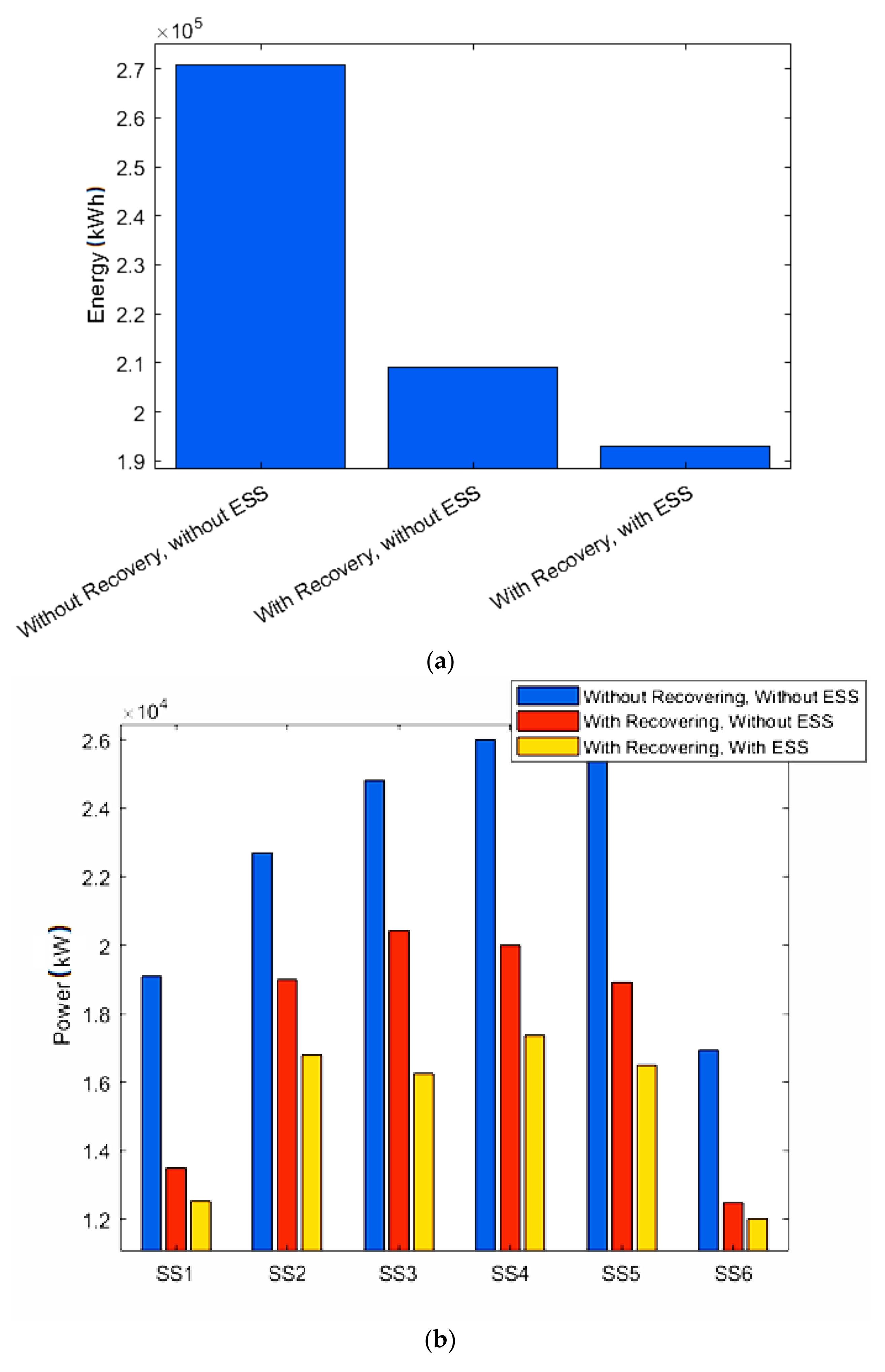
The solution provided allows to have the maximum possible profit and a relatively short payback period. Furthermore, making a comparison between the case without ESS and with ESS, less energy is drawn from the primary network and also a lower impact on the electrical substations, which are, especially those located in the middle of the line, less stressed, as shown in Figure 8b. Specifically, being able to count on the possibility of trains to reuse braking energy decreases the energy absorbed by the primary network by about 34% and the installation of an ESS along the line allows for about a further 8% less energy drawn. The electrical substations, on the other hand, thanks to the recovery of braking energy, deliver on average 30% less power (with peaks of over 40% for the substations located at the limits of the railway line), which is further lowered by about 5% in average (with peaks over 10% for the mid-line substations) thanks to the presence of ESS.
Moreover, it should be noted that through the ESS the electrical substations and the traction line are stressed less, with consequent benefits from the point of view of maintenance, aging and replacement of materials.
Even if it is not one of the specific objectives of the model, the adoption of an ESS along the line has the further benefit of reducing the system’s energy losses (31 MWh against 32.9 MWh in a standard working day).
These aspects allow considerable savings in the long period and increase the advantages that can be obtained after installation: these are not taken into account by energy savings, but are estimated in the economic model on which PSO is based, so the solution provided allows to have greater overall benefits than looking only at the energy aspect.
The operation of the line (timetable) is a fundamental role in the choice of the installation to be carried out. Using the same network and route characteristics of previous simulation, but with another timetable (only “soft” periods), it possible to appreciate that a much higher percentage of energy saving, taken into account ESS, is reached (Figure 9).
The electrical substations load is more decreased, with benefits from the point of view of maintenance and replacement, as previously mentioned, which are not directly visible in energy consumption. Being able to simulate multiple service hours, it can be seen how this characteristic of the proposed model allows for a more accurate and realistic solution.
To avoid unusable solutions and excessively long and expensive simulation times, it is advisable to choose numerical ranges that have real ESS sizes and that are not too wide.
A further strength of the software is the possibility of providing more ESSs on the line: in fact, it is possible to impose a number of accumulators greater than 1 and to obtain the optimal solution from the software with that specific configuration. A simulation performed by predicting 2 ESSs in line, with the same ranges of decision variables predicted in Table 8, led to the follow solution:
- NPV: 383,451.71 €
- Payback period: 3.6648 years
- ESSs’ position: 6 km, 55 km
- Nominal power: 0.100 MW, 0.400 MW
- Nominal energy: 0.100 MWh, 0.200 MWh
The proposed solution involves a lower NPV than the case with only one ESS installed, but looking at the graphic outputs of the software (Figure 10), comparing the case without ESSs with that with two ESSs, an energy saving of about 14% is noted (compared to 8% in the previous case). The electrical substations deliver about 9% less power on average (before it was 5%), with peaks over 15% for the mid-line substations when 2 ESSs are installed according to the proposed method.
Also, from the point of view of the energy losses of the system, the solution proposed with two ESSs installed results in lower losses compared to the previous case with only one ESS installed (29.3 MWh against 31 MWh in a standard working day).
Despite a lower economic return from the installation, i.e. a slightly lower but still positive NPV, it is possible to lighten the electrical substations and draw even less energy from the network. The user who manages the software can evaluate the benefits of this solution through the graphic output, that allows to have all the information, both technical and economic, of the installation to be carried out.
4. Discussion
The results obtained show how the proposed solution allows an effective economic return on investment. From an economic point of view, also as regards the energy one, it allows savings percentages comparable to those obtained from [7] and [25], but with the advantage of having stationary installations that don’t burden the convoys. The PBP turns out to be greater than that found by our model since in [25] the economic aspect of the problem is a sub-objective, not the main one and therefore is not maximized.
Compared to other research based on single types of accumulation [16,20,21,23] by varying the parameters characterizing the different types within the model it is possible to consider different ESSs, and the different investments can be compared with each other by means of a single value, which is the NPV.
The use of this parameter also allows, as seen, to evaluate cases with different numbers of ESS installed, which entail different energy savings (shown to the user) but in any case, comparable from an economic point of view through the NPV. Comparing different scenarios is a possibility also offered by [30] but it needs real traffic data: the use of the railway simulator instead allows to simulate countless traffic scenarios only by knowing the characteristics of the line and those of the rolling stock. The model takes into account the management of the line and offers different solutions based on its use.
The economic model described in Section 2.3 in the evaluation of the NPV examines the charge and discharge cycles of the ESS as [24], which bases its optimization on this parameter. The solution found by our model is therefore based on a greater number of variables and this allows for a more in-depth and realistic solution.
Further developments in the sector could involve an ever-greater integration between technical and economic design, using multi-objective optimization to simultaneously maximize or minimize technical aspects (e.g. energy losses or system receptivity) and economic aspects (e.g. the capital cost of the investment or the expected economic returns). Modified and more complex models should be adopted to effectively describe the reciprocal influence between the two aspects mentioned above.
From the point of view of railway safety, many studies [42,43,44,45,46,47,48,49] have recently been conducted on the safety of the infrastructure and on the effects that accidents and derailments have on it and on its deterioration. The addition of ESSs on the line involves new variables whose effects should be deepened.
Furthermore, it would be interesting to be able to compare other solutions, such as on-board storage systems or the installation of reversible electrical substations, with those found. Common models should be developed for the different types of proposed solutions in which future technological developments can also be taken into account.
The proposed methodology can be further developed by providing for the inclusion in the model of constraints related to the exchange of energy or by inserting a limit on the energy consumed in order to have lower energy consumption and less stress on the electrical substations. Other solutions to explore include: the replacement of the PSO with derivative-free algorithms of “pattern search” type, based on the guided exploration of the feasible region; instead of the railway simulator, use non-parametric machine learning models derived from the data collected or simulated on the network. In the last case, it would apply algorithms which use the derivatives and that are more advanced and efficient for the determination of the optimal solution or one of its good approximation.
Since the installation of an ESS involves a very expensive investment, the initial choice of the type of storage is an important problem: in fact, the rates of the economic parameters change according to the technology used and this means that, for the same installed size, different technologies involve different costs and therefore also different economic benefits. The proposed methodology allows to take into account the impact of the various rates, i.e., the various technologies that can be installed, since the economic model used by the algorithm to calculate the NPV of the system depends on economic parameters that change according to the technology adopted, therefore by changing the parameters’ values of ESS it is possible to obtain a different economic calculation and a different optimal solution, depending on the chosen technology.
5. Conclusions
This paper proposes a methodology to determine the optimal siting and sizing of energy storage systems along railway lines: the results found show how the proposed approach maximizes the economic return on investment required to install an ESS along a railway line. Using the PSO it is possible to obtain a faster solution than other meta-heuristic algorithms. Using the NPV and the PBP, used by the analysis of investments in financial mathematics, it is possible to directly compare two alternative investments with the same risk profile, thus obtaining a more realistic assessment of the feasibility and convenience of the installation.
The proposed method can be used for any type of d.c. electrified railway line, it can model any existing rolling stock and allows to simulate multiple working timetables and the simultaneous presence of multiple ESSs. In this way it is possible to find the optimal equipment for countless ESSs’ installations located along a railway line through a model that is also easy to use.
Author Contributions
Conceptualization, R.L., L.P. and A.R.; methodology, N.M.; software, N.M.; validation, L.P.; formal analysis, N.M.; investigation, N.M.; data curation, N.M. and A.R.; writing—original draft preparation, N.M.; writing—review and editing, R.L. and A.R.; visualization, N.M.; supervision, R.L. and A.R. All authors have read and agreed to the published version of the manuscript.
Funding
This research received no external funding.
Conflicts of Interest
The authors declare no conflict of interest.
Abbreviations
| Capital cost of the ESS (€) | |
| n | Generic year during the life of the ESS (-) |
| N | Useful life (in years) of the ESS (-) |
| Cash flow of the year “n” (€) | |
| Income of the year “n” (€) | |
| Expenses of the year “n” (€) | |
| Total days of use of the ESS within one year (-) | |
| Number of peak periods per day (-) | |
| Number of soft periods per day (-) | |
| Total energy withdrawn from the primary network, without ESSs in the track, in the year “n” (kWh) | |
| Total energy withdrawn from the primary network, with ESSs in the track, in the year “n” (kWh) | |
| Total energy withdrawn from the primary network, without ESSs in the track, in one working day (kWh) | |
| Total energy withdrawn from the primary network, without ESSs in the track, in one working day (kWh) | |
| Total energy withdrawn from the primary network during the peak period, without ESSs in the track (kWh) | |
| Total energy withdrawn from the primary network during the soft period, without ESSs in the track (kWh) | |
| Total energy withdrawn from the primary network during the peak period, with ESSs in the track (kWh) | |
| Total energy withdrawn from the primary network during the soft period, with ESSs in the track (kWh) | |
| Cost of electricity coefficient (€/kWh) | |
| Fixed costs of the ESS (€/kW) | |
| PBP | Payback Period (in years) of the ESS (-) |
| Nominal power of the ESS (MW) | |
| Variable costs of the ESS (€/kWh) | |
| Total energy supplied by the ESS in a working day (kWh) | |
| Energy supplied by the ESS during the peak period (kWh) | |
| Energy supplied by the ESS during the soft period (kWh) | |
| Average value of the battery charging efficiency (-) | |
| Specific cost of battery power (€/kW) | |
| Specific cost of battery energy (€/kWh) | |
| Nominal energy of the ESS (MWh) | |
| Future value of replacement cost (€) | |
| Future value of the battery (assumed to be equal to the capital cost of the battery) (€) | |
| Interest rate (-) | |
| Battery replacement period (in years) (-) | |
| Useful life (in years) of the batteries (-) | |
| NPV | Net present value |
| Number of times the battery must be replaced during the life of the ESS (-) |
References
- European Comission. EU Energy, Transport and GHG Emissions Trends to 2050, Reference Scenario 2016. Available online: http://ec.europa.eu/energy (accessed on 26 November 2020).
- Aguado, J.A.; Sánchez Racero, A.J.; de la Torre, S. Optimal Operation of Electric Railways with Renewable Energy and Electric Storage Systems. IEEE Trans. Smart Grid 2018, 9, 993–1001. [Google Scholar] [CrossRef]
- Lamedica, R.; Ruvio, A.; Papalini, A.; Spalvieri, C.; Rossetta, I. Train braking impact on energy recovery: The case of the 3 kV d.c. railway line Roma-Napoli via Formia. In Proceedings of the 2019 AEIT International Annual Conference, Florence, Italy, 18–20 September 2019; pp. 1–6. [Google Scholar]
- Su, S.; Tang, T.; Wang, Y. Control of urban rail transit equipped with ground-based supercapacitor for energy saving and reduction of power peak demand. Energies 2016, 9, 1–19. [Google Scholar]
- Lamedica, R.; Ruvio, A.; Galdi, V.; Graber, G.; Sforza, P.; Guidi Buffarini, G.; Spalvieri, C. Application of Battery Auxiliary Substations in 3kV Railway Systems. In Proceedings of the 2015 AEIT International Annual Conference, Naples, Italy, 14–16 October 2015; pp. 1–6. [Google Scholar]
- Gao, Z.; Fang, J.; Zhang, Y.; Jiang, L.; Sun, D.; Guo, W. Evaluation of strategies to reducing traction energy consumption of metro systems using an Optimal Train Control Simulation model. Int. J. Elec. Power 2015, 67, 439–447. [Google Scholar] [CrossRef]
- Kampeerawat, W.; Toseki, T. Integrated design of smart train scheduling, use of onboard energy storage, and traction power management for energy-saving urban railway operation. IEEJ J. Ind. Appl. 2019, 8, 893–903. [Google Scholar] [CrossRef]
- Wu, C.; Lu, S.; Xue, F.; Jiang, L.; Chen, M. Optimal Sizing of Onboard Energy Storage Devices for Electrified Railway Systems. IEEE Trans. Transport. Electrific. 2020, 6, 1301–1311. [Google Scholar] [CrossRef]
- Popescu, M.; Bitoleanu, A. A Review of the Energy Efficiency Improvement in DC Railway Systems. Energies 2019, 12, 1092. [Google Scholar] [CrossRef] [Green Version]
- Meinert, M. New mobile energy storage system for rolling stock. In Proceedings of the 2009 European Conference on Power Electronics and Applications, Barcelona, Spain, 8–10 September 2009; pp. 1–10. [Google Scholar]
- Kampeerawat, W.; Toseki, T. Efficient urban railway design integrating train scheduling, wayside energy storage, and traction power management. IEEJ J. Ind. Appl. 2019, 8, 915–925. [Google Scholar] [CrossRef]
- Barsali, S.; Bechini, A.; Giglioli, R.; Poli, D. Storage in electrified transport systems. In Proceedings of the 2012 IEEE International Energy Conference and Exhibition, Florence, Italy, 9–12 September 2012; pp. 1003–1008. [Google Scholar]
- Hanmin, L.; Gildong, K.; Changmu, L.; Euijin, J. Field tests of DC 1500 V stationary energy storage system. Int. J. Railway 2012, 5, 124–128. [Google Scholar]
- Ratniyomchai, T.; Kulworawanichpong, T. A Demonstration Project for Installation of Battery Energy Storage System in Mass Rapid Transit. Energy Procedia 2017, 138, 93–98. [Google Scholar] [CrossRef]
- Barrero, R.; Tackoen, X.; Van Mierlo, J. Stationary or onboard energy storage systems for energy consumption reduction in a metro network. Proc. Inst. Mech. Eng. F J. Rail Rapid Transit 2010, 224, 207–225. [Google Scholar] [CrossRef]
- Gee, A.M.; Dunn, R.W. Analysis of trackside flywheel energy storage in light rail systems. IEEE Trans. Veh. Technol. 2015, 64, 3858–3869. [Google Scholar] [CrossRef]
- Lee, H.; Song, J.; Jang, G.; Kim, G.; Lee, H.; Lee, C. Capacity optimization of the supercapacitor energy storages on DC railway system using a railway powerflow algorithm. Int. J. Innov. Comput. I. 2011, 7, 2739–2753. [Google Scholar]
- Ratniyomchai, T.; Hillmansen, S.; Tricoli, P. Optimal capacity and positioning of stationary supercapacitors for light rail vehicle systems. In Proceedings of the 2014 International Symposium on Power Electronics, Electrical Drives, Automation and Motion, Ischia, Italy, 18–20 June 2014; pp. 807–812. [Google Scholar]
- Battistelli, L.; Ciccarelli, F.; Lauria, D.; Proto, D. Optimal design of DC electrified railway stationary storage system. In Proceedings of the 2009 International Conference on Clean Electrical Power, Capri, Italy, 9–11 June 2009; pp. 739–745. [Google Scholar]
- Ratniyomchai, T.; Hillmansen, S.; Tricoli, P. Energy loss minimisation by optimal design of stationary supercapacitors for light railways. In Proceedings of the 2015 International Conference on Clean Electrical Power, Taormina, Italy, 16–18 June 2015; pp. 511–517. [Google Scholar]
- Calderaro, V.; Galdi, V.; Graber, G.; Piccolo, A. Optimal siting and sizing of stationary supercapacitors in a metro network using PSO. In Proceedings of the 2015 IEEE International Conference on Industrial Technology, Seville, Spain, 17–19 March 2015; pp. 1–6. [Google Scholar]
- Xia, H.; Chen, H.; Yang, Z.; Lin, F.; Wang, B. Optimal Energy Management, Location and Size for Stationary Energy Storage System in a Metro Line Based on Genetic Algorithm. Energies 2015, 8, 11618–11640. [Google Scholar] [CrossRef]
- Graber, G.; Calderaro, V.; Galdi, V.; Piccolo, A.; Lamedica, R.; Ruvio, A. Techno-economic Sizing of Auxiliary-Battery-Based Substations in DC Railway Systems. IEEE T. Transp. Electr. 2018, 4, 616–625. [Google Scholar] [CrossRef]
- De la Torre, S.; Sanchez-Racero, A.J.; Aguado, J.A.; Reyes, M.; Martianez, O. Optimal Sizing of Energy Storage for Regenerative Braking in Electric Railway Systems. IEEE Trans. Power Syst. 2015, 30, 1492–1500. [Google Scholar] [CrossRef]
- Wang, B.; Yang, Z.; Lin, F.; Zhao, W. An improved genetic algorithm for optimal stationary energy storage system locating and sizing. Energies 2014, 7, 6434–6458. [Google Scholar] [CrossRef] [Green Version]
- Li, Y.; Wang, J.; Gu, C.; Liu, J.; Li, Z. Investment optimization of grid-scale energy storage for supporting different wind power utilization levels. J. Mod. Power Syst. Clean Energy 2019, 7, 1721–1734. [Google Scholar] [CrossRef] [Green Version]
- Yuan, Z.; Wang, W.; Wang, H.; Yildizbasi, A. A new methodology for optimal location and sizing of battery energy storage system in distribution networks for loss reduction. J. Energy Storage 2020, 29, 101368. [Google Scholar] [CrossRef]
- Miao, D.; Hossain, S. Improved gray wolf optimization algorithm for solving placement and sizing of electrical energy storage system in micro-grids. ISA Trans. 2020, 102, 376–387. [Google Scholar] [CrossRef]
- Kerdphol, T.; Fuji, K.; Mitani, Y.; Watanabe, M.; Qudaih, Y. Optimization of a battery energy storage system using particle swarm optimization for stand-alone microgrids. Int. J. Elec. Power. 2016, 81, 32–39. [Google Scholar] [CrossRef]
- Yoshida, Y.; Figueroa, H.P.; Dougal, R.A. Use of Time Series Load Data to Size Energy Storage Systems. In Proceedings of the 2018 IEEE Green Energy and Smart Systems Conference, Long Beach, CA, USA, 29–30 October 2018; pp. 1–6. [Google Scholar]
- Pandey, A.K.; Kirmani, S. Optimal location and sizing of hybrid system by analytical crow search optimization algorithm. Int. Trans. Electr. Energy Syst. 2020, 30, e12327. [Google Scholar] [CrossRef]
- Ruiyang, J.; Jie, S.; Jie, L.; Wei, L.; Chao, L. Location and Capacity Optimization of Distributed Energy Storage System in Peak-Shaving. Energies 2020, 13, 513. [Google Scholar]
- Rajamand, S. Loss cost reduction and power quality improvement with applying robust optimization algorithm for optimum energy storage system placement and capacitor bank allocation. Int. J. Energy Res. 2020, 44, 11973–11984. [Google Scholar] [CrossRef]
- Lata, P.; Vadhera, S. TLBO-based approach to optimally place and sizing of energy storage system for reliability enhancement of radial distribution system. Int. Trans. Electr. Energ. Syst. 2020, 30, e12334. [Google Scholar] [CrossRef]
- Davis, E. Solving MINLP containing noisy variables and black-box functions using Branch-and-Bound. Comput. Aided Chem. Eng. 2006, 21, 633–638. [Google Scholar]
- Calderaro, V.; Galdi, V.; Graber, G.; Piccolo, A. Deterministic vs. Heuristic Algorithms for Eco-Driving Application in Metro Network. In Proceedings of the 2015 International Conference on Electrical Systems for Aircraft, Railway, Ship Propulsion and Road Vehicles, Aachen, Germany, 3–5 March 2015; pp. 1–6. [Google Scholar]
- Capasso, A.; Lamedica, R.; Ruvio, A.; Giannini, G. Eco-friendly urban transport systems. Comparison between energy demands of the trolleybus and tram systems. Ing. Ferrov. 2014, 69, 329–347. [Google Scholar]
- Capasso, A.; Lamedica, R.; Ruvio, A.; Ceraolo, M.; Lutzemberger, G. Modelling and simulation of electric urban transportation systems with energy storage. In Proceedings of the 2016 IEEE 16th International Conference on Environment and Electrical Engineering, Florence, Italy, 7–10 June 2016; pp. 1–5. [Google Scholar]
- Lamedica, R.; Gatta, F.M.; Geri, A.; Sangiovanni, S.; Ruvio, A. A software validation for dc electrified transportation system: A tram line of Rome. In Proceedings of the 2018 IEEE International Conference on Environment and Electrical Engineering and 2018 IEEE Industrial and Commercial Power Systems Europe, Palermo, Italy, 12–15 June 2018; pp. 1–6. [Google Scholar]
- Poonpun, P.; Jewell, W.T. Analysis of the cost per kilowatt hour to store electricity. IEEE Trans. Energy Convers. 2008, 23, 529–534. [Google Scholar] [CrossRef]
- Del Valle, Y.; Venayagamoorthy, G.K.; Mohagheghi, S.; Hernandez, J.C.; Harley, R.G. Particle Swarm Optimization: Basic Concepts, Variants and Applications in Power Systems. IEEE T. Evolut. Comput. 2008, 12, 171–195. [Google Scholar] [CrossRef]
- Dindar, S.; Kaewunruen, S.; An, M. Identification of appropriate risk analysis techniques for railway turnout systems. J. Risk Res. 2018, 21, 974–995. [Google Scholar] [CrossRef]
- Alawad, H.; Kaewunruen, S.; An, M. Learning from Accidents: Machine Learning for Safety at Railway Stations. IEEE Access. 2020, 8, 633–648. [Google Scholar] [CrossRef]
- Kaewunruen, S.; Bin Osman, M.H.; Wong, H.C.E. Risk-based maintenance planning for rail fastening systems. ASCE ASME J. Risk Uncertain. Eng. Syst. A Civ. Eng. 2019, 5, 04019007. [Google Scholar] [CrossRef] [Green Version]
- Kampczyk, A. Measurement of the Geometric Center of a Turnout for the Safety of Railway Infrastructure Using MMS and Total Station. Sensors 2020, 20, 4467. [Google Scholar] [CrossRef] [PubMed]
- Wang, H.; Chang, L.; Markine, V.L. Structural Health Monitoring of Railway Transition Zones Using Satellite Radar Data. Sensors 2018, 18, 413. [Google Scholar] [CrossRef] [PubMed] [Green Version]
- Guo, Y.; Zhao, C.; Markine, V.L.; Jing, G.; Zhai, W. Calibration for discrete element modelling of railway ballast: A review. Transp. Geotech. 2020, 23, 100341. [Google Scholar] [CrossRef]
- Dindar, S.; Kaewunruen, S.; An, M. Rail accident analysis using large-scale investigations of train derailments on switches and crossings: Comparing the performances of a novel stochastic mathematical prediction and various assumptions. Eng. Fail. Anal. 2019, 103, 203–216. [Google Scholar] [CrossRef]
- Ye, Y.; Shi, D.; Poveda-Reyes, S.; Hecht, M. Quantification of the influence of rolling stock failures on track deterioration. J. Zhejiang Univ. Sci. A 2020, 21, 783–798. [Google Scholar] [CrossRef]
Figure 1.
Recovery of braking energy: (a) reversible substations (RSSs); (b) energy storage systems (ESSs).
Figure 1.
Recovery of braking energy: (a) reversible substations (RSSs); (b) energy storage systems (ESSs).
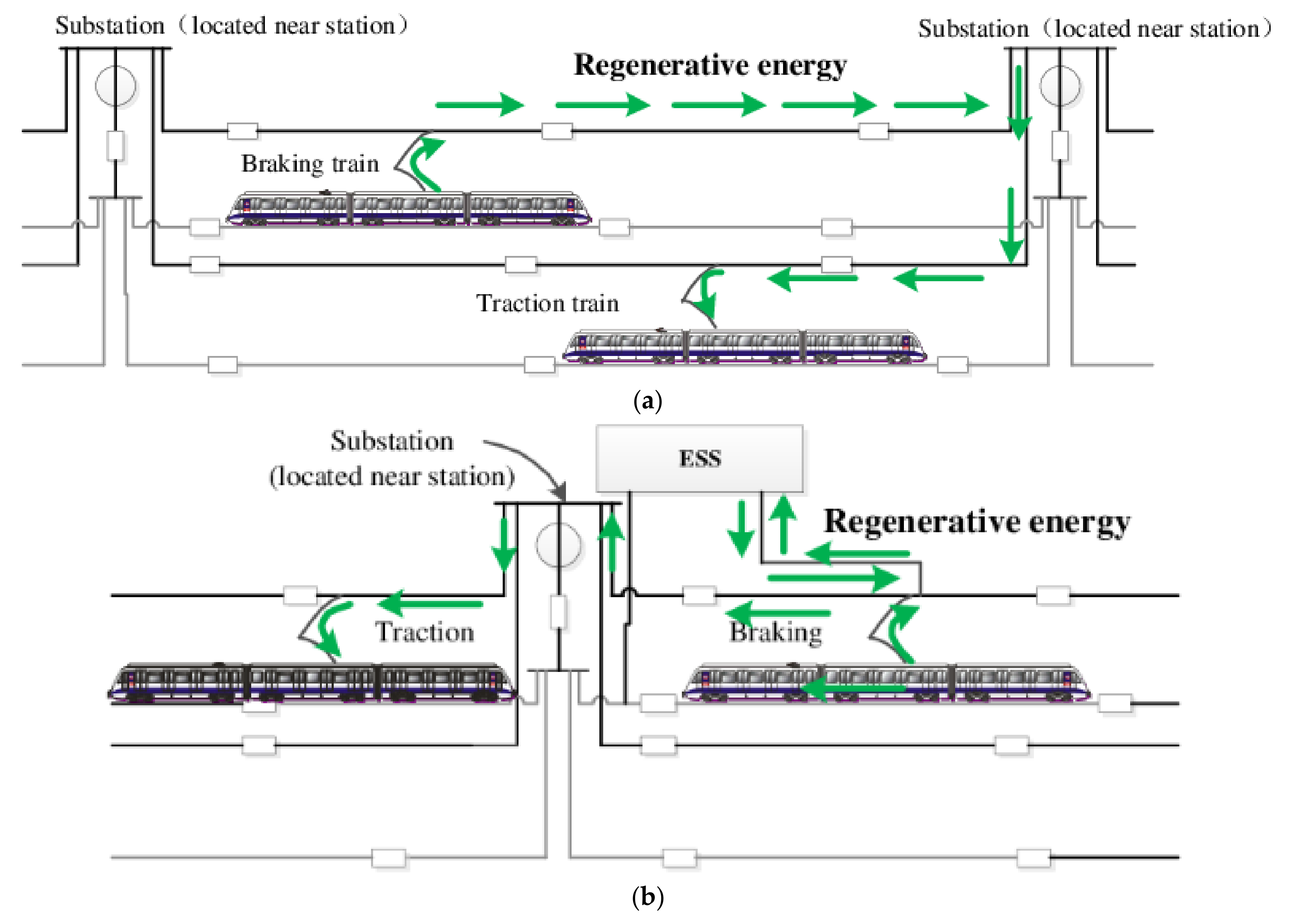
Figure 2.
V-I characteristic of a typical electric substation.
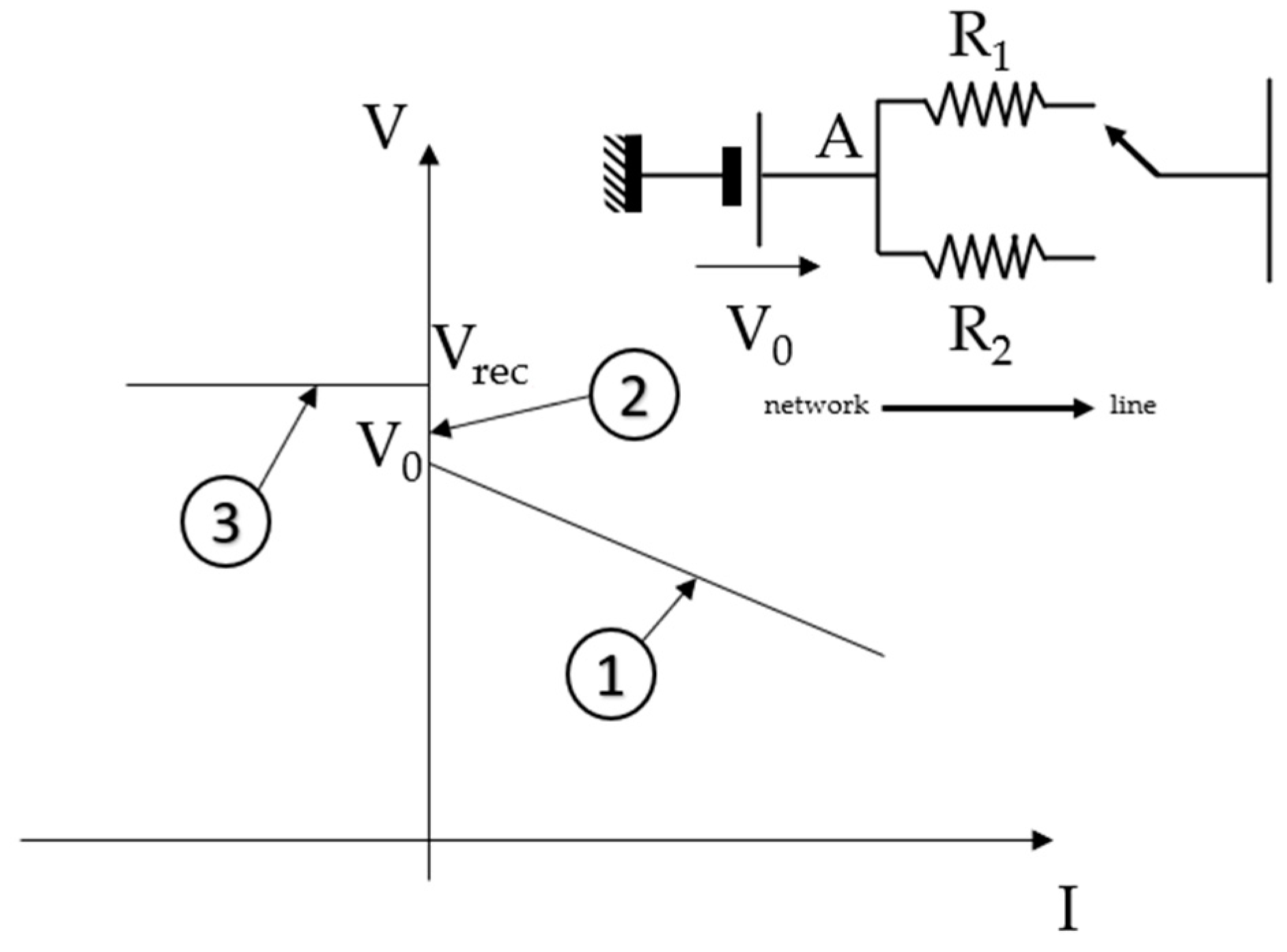
Figure 3.
V-P characteristic of traction vehicles.

Figure 4.
Flowchart of the PSO-based solution algorithm.
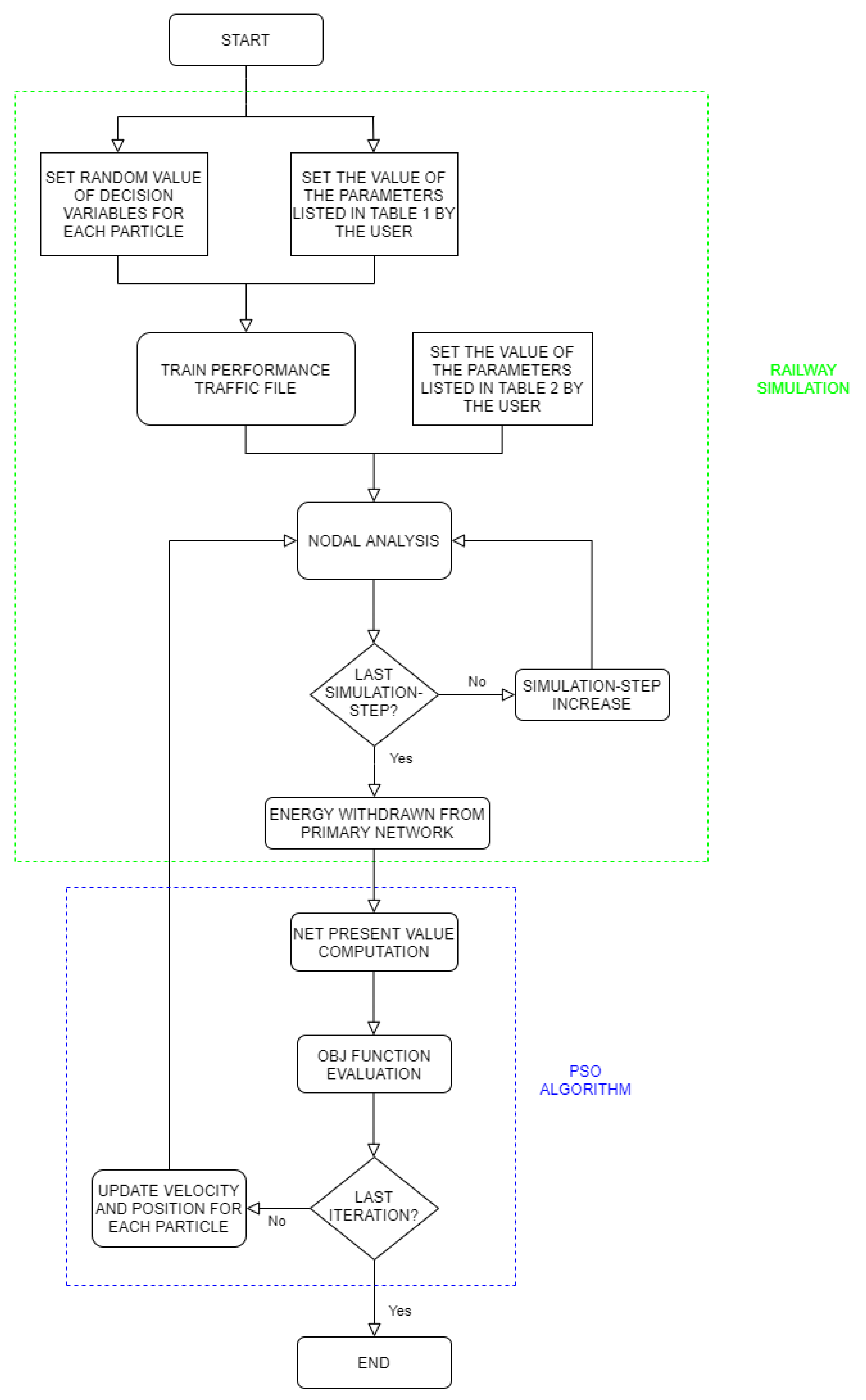
Figure 5.
Characteristics of the railway line.
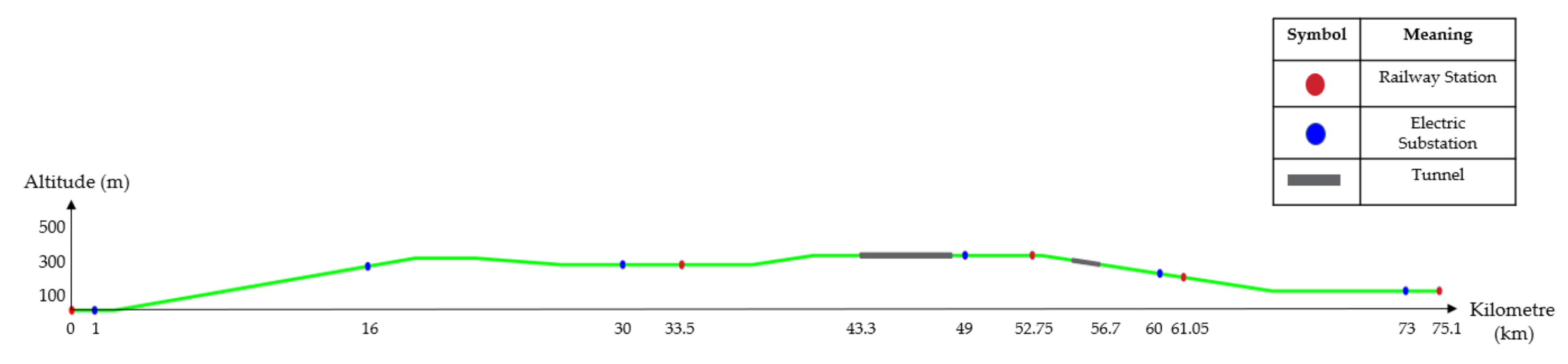
Figure 6.
Slope of line.
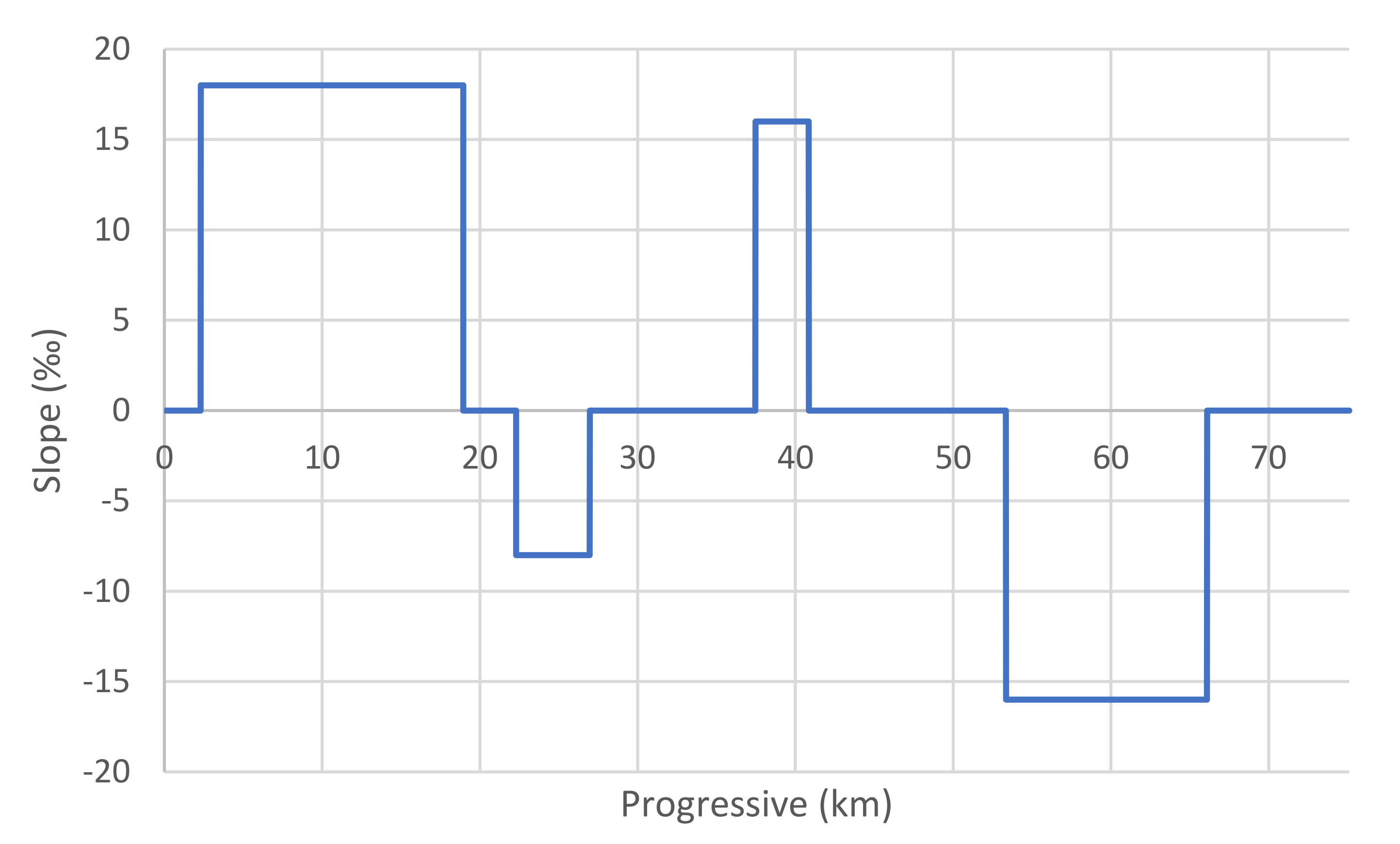
Figure 7.
Speed cycle of the train.
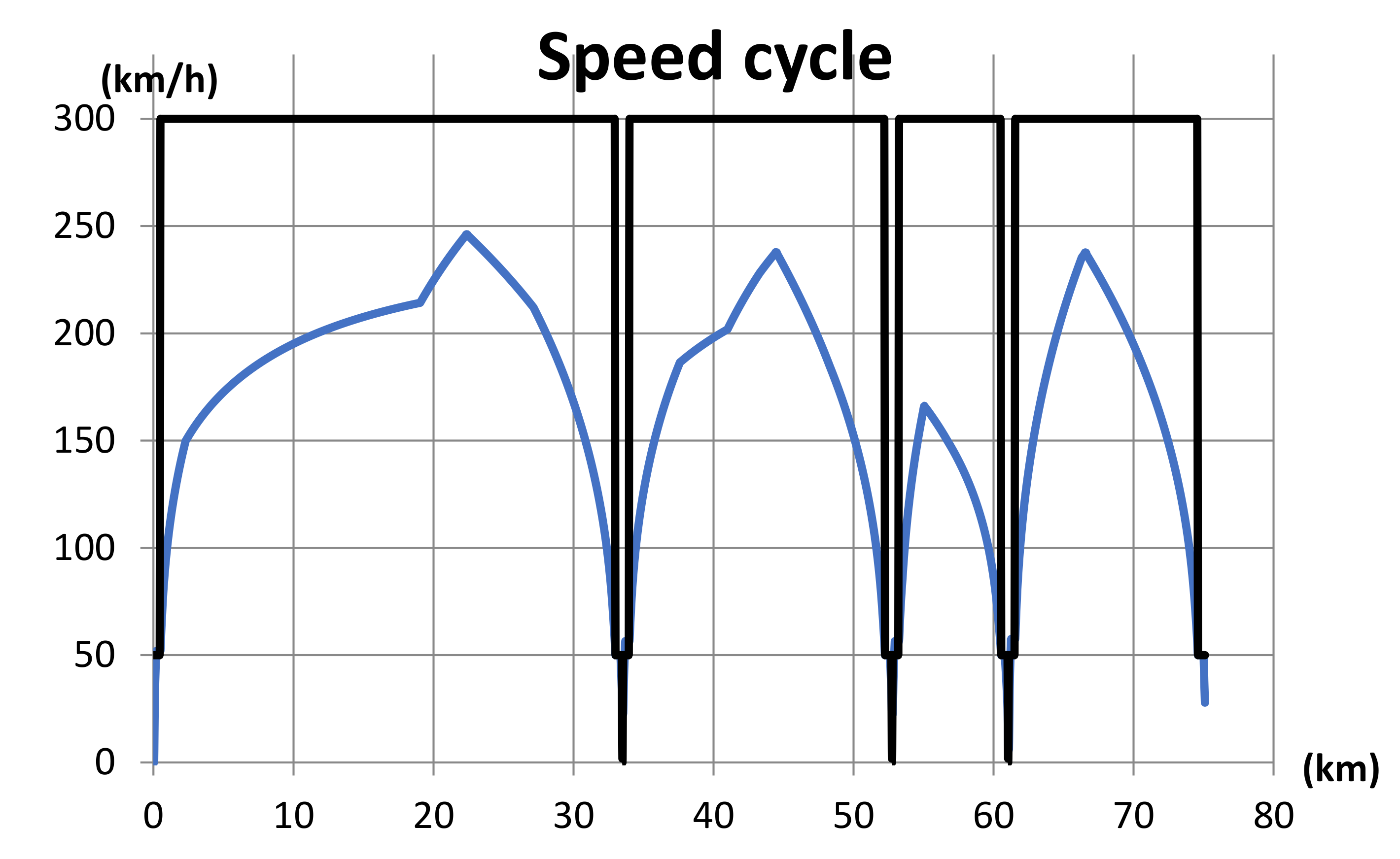
Figure 8.
Graphic software output: (a) Total energy withdrawn from the primary network in a working day; (b) Power supplied by each substation present on the line.
Figure 8.
Graphic software output: (a) Total energy withdrawn from the primary network in a working day; (b) Power supplied by each substation present on the line.
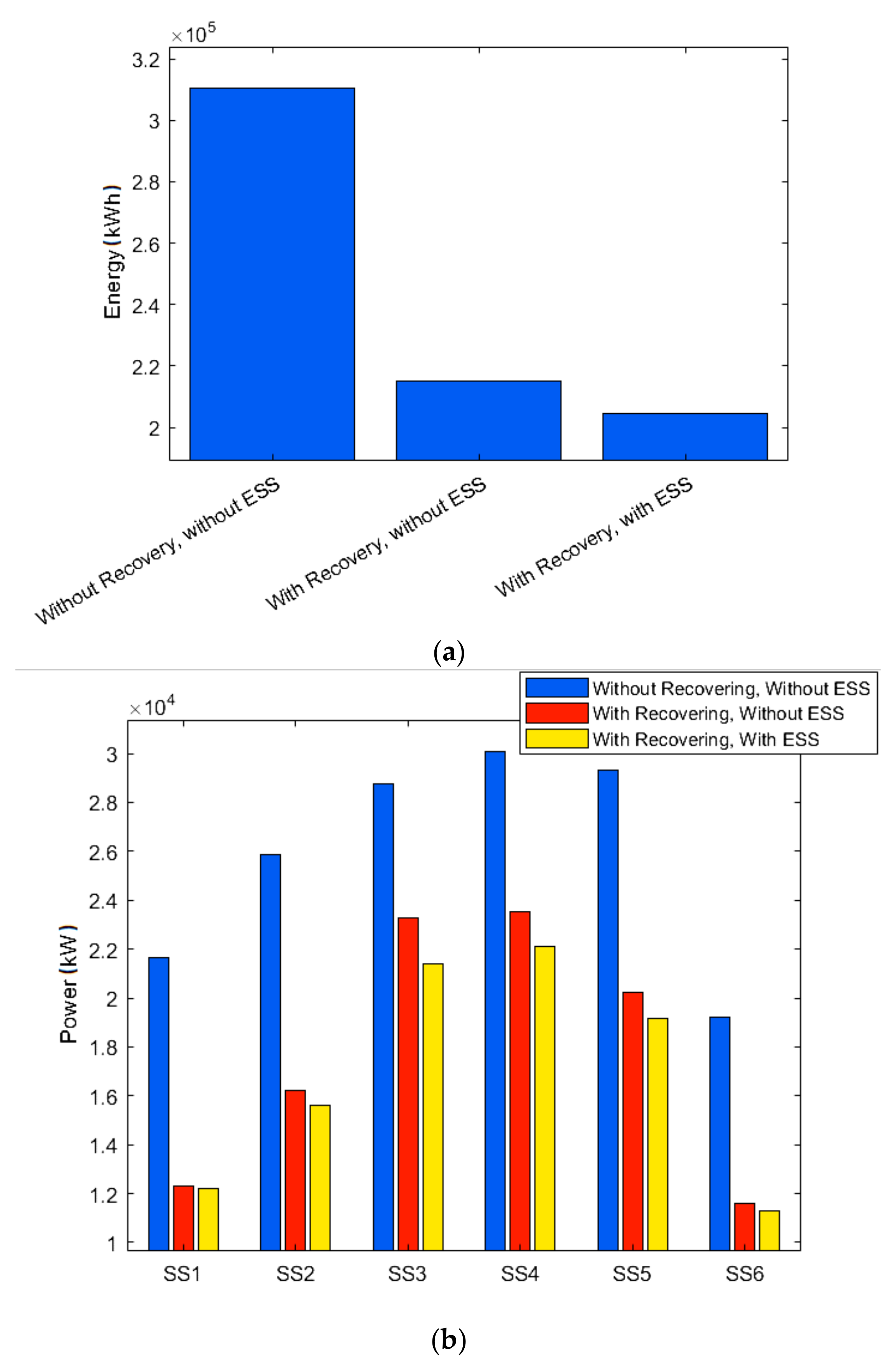
Figure 9.
Graphic software output: (a) Total energy withdrawn from the primary network in a working day; (b) Power supplied by each substation present on the line.
Figure 9.
Graphic software output: (a) Total energy withdrawn from the primary network in a working day; (b) Power supplied by each substation present on the line.
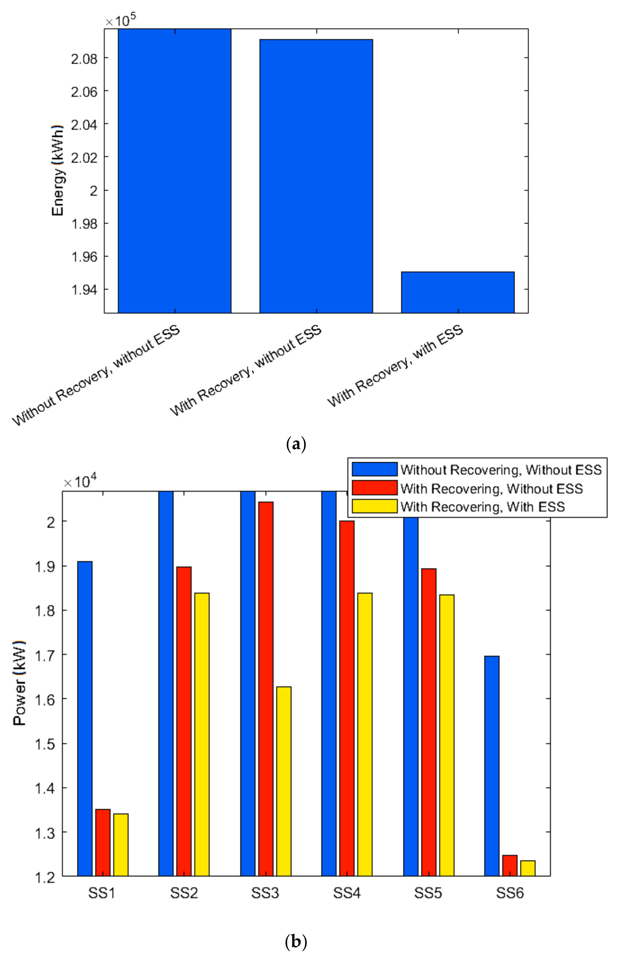
Figure 10.
Graphic software output with 2 ESSs on the route: (a) Total energy withdrawn from the primary network in a working day; (b) Power supplied by each substation present on the line.
Figure 10.
Graphic software output with 2 ESSs on the route: (a) Total energy withdrawn from the primary network in a working day; (b) Power supplied by each substation present on the line.

Table 1.
Inputs and outputs of train performance simulation.
| Characteristics of the Route (Inputs) | Characteristics of the Vehicle (Inputs) | Values Every 15 Seconds (Outputs) |
|---|---|---|
| Progressive | Aerodynamic resistance | Pantograph power |
| Slopes Curves Tunnels Speed limits | Traction force Braking force Weight | Distance |
Table 2.
Inputs and outputs of traction system simulation.
| Electrical Inputs | Outputs |
|---|---|
| Number and kilometric point of substations | Instantaneous powers required to substations |
| Number and type of transformer-rectifier units | Voltage at the vehicle pantographs, at substation bars and at parallel points |
| Catenary feature | Line minimum instantaneous voltages |
| Line rated, minimum and maximum voltage | Current on substation feeders and in traction circuit branches |
| Traffic Input | Recovered energy on line |
| Train performance traffic file | Power losses in traction circuit |
| Recovered energy in the network Energy storage operating profile |
Table 3.
Position of the stations.
| Station Name | Progressive (km) |
|---|---|
| Departure station | 0 |
| Intermediate station #1 | 33.5 |
| Intermediate station #2 | 52.75 |
| Intermediate station #3 | 61.05 |
| Arrival station | 75.1 |
Table 4.
Tunnels’ position.
| Tunnel Name | Length (km) | From (km) | To (km) |
|---|---|---|---|
| Tunnel #1 | 5 | 43.3 | 48.3 |
| Tunnel #2 | 1.5 | 55.2 | 56.7 |
Table 5.
Substations on the line.
| Substation Name | Conversion Units | Nominal Power (MW) | Progressive (km) |
|---|---|---|---|
| Electric substation #1 | 2 | 5.4 | 1 |
| Electric substation #2 | 2 | 5.4 | 16 |
| Electric substation #3 | 2 | 5.4 | 30 |
| Electric substation #4 | 2 | 5.4 | 45 |
| Electric substation #5 | 2 | 5.4 | 60 |
| Electric substation #6 | 2 | 5.4 | 73 |
Table 6.
Rolling stock data.
| Parameter | Value | |
|---|---|---|
| Loaded weight | 500 | t |
| Rotating mass coefficient | 0.05 | |
| Motor efficiency | 0.85 | |
| Auxiliaries power | 400 | kW |
| Full speed | 360 | km/h |
| Maximum traction effort | 370 | kN |
| Maximum deceleration | 0.6 | m/s2 |
Table 7.
Service hours.
| From (hh:mm) | To (hh:mm) | Band |
|---|---|---|
| 07:00 | 09:00 | Peak |
| 09:00 | 11:00 | Soft |
| 11:00 | 13:00 | Soft |
| 13:00 | 15:00 | Peak |
| 15:00 | 17:00 | Soft |
| 17:00 | 19:00 | Peak |
| 19:00 | 21:00 | Soft |
| 21:00 | 23:00 | Soft |
Table 8.
Economic inputs.
| Parameters | Values | Unit |
|---|---|---|
| Cp | 120 | €/kW |
| CE | 440 | €/kWh |
| Cf | 7.2 | €/kW |
| Cv | 0.0011 | €/kWh |
| Cch | 0.015 | €/kWh |
| N | 20 | #years |
| ɳCH | 0.90 | - |
Table 9.
Input parameters of the optimization algorithm.
| Variables of Decision | Lower Bound | Upper Bound |
|---|---|---|
| Position (km) | 0 | 75.1 |
| Nominal power (MW) | 0.1 | 1 |
| Nominal energy (MWh) | 0.1 | 1 |
Publisher’s Note: MDPI stays neutral with regard to jurisdictional claims in published maps and institutional affiliations. |
© 2020 by the authors. Licensee MDPI, Basel, Switzerland. This article is an open access article distributed under the terms and conditions of the Creative Commons Attribution (CC BY) license (http://creativecommons.org/licenses/by/4.0/).
Share and Cite
MDPI and ACS Style
Lamedica, R.; Ruvio, A.; Palagi, L.; Mortelliti, N. Optimal Siting and Sizing of Wayside Energy Storage Systems in a D.C. Railway Line. Energies 2020, 13, 6271. https://doi.org/10.3390/en13236271
AMA Style
Lamedica R, Ruvio A, Palagi L, Mortelliti N. Optimal Siting and Sizing of Wayside Energy Storage Systems in a D.C. Railway Line. Energies. 2020; 13(23):6271. https://doi.org/10.3390/en13236271
Chicago/Turabian StyleLamedica, Regina, Alessandro Ruvio, Laura Palagi, and Nicola Mortelliti. 2020. "Optimal Siting and Sizing of Wayside Energy Storage Systems in a D.C. Railway Line" Energies 13, no. 23: 6271. https://doi.org/10.3390/en13236271
Note that from the first issue of 2016, this journal uses article numbers instead of page numbers. See further details here.