Robust Economic Model Predictive Control Based on a Zonotope and Local Feedback Controller for Energy Dispatch in Smart-Grids Considering Demand Uncertainty ^†

Abstract

Electrical smart grids are complex MIMO systems whose operation can be noticeably affected by the presence of uncertainties such as load demand uncertainty. In this paper, based on a restricted representation of the demand uncertainty, we propose a robust economic model predictive control method that guarantees an optimal energy dispatch in a smart micro-grid. Load demands are uncertain, but viewed as bounded. The proposed method first decomposes control inputs into dependent and independent components, and then tackles the effect of demand uncertainty by tightening the system constraints as the uncertainty propagates along the prediction horizon using interval arithmetic and local state feedback control law. The tightened constraints’ upper and lower limits are computed off-line. The proposed method guarantees stability through a periodic terminal state constraint. The method is faster and simpler compared to other approaches based on Closed-loop min–max techniques. The applicability of the proposed approach is demonstrated using a smart micro-grid that comprises a wind generator, some photovoltaic (PV) panels, a diesel generator, a hydroelectric generator and some storage devices linked via two DC-buses, from which load demands can be adequately satisfied.

1. Introduction

The most trivial approach of tackling uncertainties is simply to neglect them i.e., to consider only the nominal system, and rely on the receding horizon control principle of MPC, which introduces a Closed-loop mechanism that could minimize the effects of uncertain disturbances. Unfortunately, there is no guarantee of achieving an optimal and stable control system in the presence of uncertainties. Therefore, it is quite necessary that, some well-thought control strategies have to be developed. Without advanced predictive control strategies, it is quite unrealistic to achieve optimal control of complex Multiple Input Multiple Output (MIMO) interconnected electrical systems such as smart grids. Many previous works [1,2,3,4] have used stochastic approaches to deal with uncertainties in generalized flow-based networks. In this study, we consider a deterministic approach namely robust optimization for tackling load demand uncertainty. Model Predictive Control (MPC) [5,6,7,8] has become nowadays one of the most sophisticated and regularly used techniques for performing optimal control of complex MIMO systems. Furthermore, uncertainties and noise can tremendously increase the complexity of smart electrical grids [9,10]. Computational constraints as reported in [11,12,13] can be enforced to tackle model uncertainty and noise. But, the issue of tractability is often of concern in this approach. Optimization techniques such as min–max MPC approaches as discussed in [14,15,16,17,18,19] can better tackle uncertainties in electrical smart grids. However, one of the main disadvantages of min–max approaches is that, they principally concentrate on worst-case scenarios. Furthermore, [13,20] have proposed some adjustable robust solutions, which assume that there exists an affine dependence between some adjustable control inputs and the uncertainty parameters of the problem. This approach is more flexible, and it is usually expected to produce a computationally tractable problem [21]. Tube-based robust MPC [22] This approach uses an independent nominal model of the system, and a feedback controller to ensure that the actual state converges to the nominal state. It is important to notice that, the optimization is made over the nominal system whose constraints are dynamically tightened with the help of robust positively control invariant sets. After that the nominal computed control inputs are adjusted using a linear feedback controller. One of its drawbacks is the requirement of a robust positively invariant set. Constraint Tightening MPC [23] This method is based on the idea of widening the state constraints, so that a trajectory can be found under any evolution of the disturbance. There is no need to compute a robustly invariant terminal constraint set. This approach might be computationally expensive. Feedback min–max MPC [24] To tackle the drawbacks of Open-loop min–max MPC, a feedback min–max MPC has been proposed. This approach is based on the idea of steering the system to a robust control invariant set using min–max MPC. Once the state is in the control invariant set Xf, a linear state feedback can be applied to adjust the control input. The method assumes that the objective function of the optimization problem is convex and zero for any state inside the control invariant set. Stability is guaranteed by using the control invariant set Xf as a terminal state constraint. The main drawback of this method is that it leads to a control law that is more computationally intensive. However, the computational load can be significantly reduced if the system is linear and the constraints are convex. Moreover, if the disturbance set is polytope, then it is sufficient to only consider the worst-case realizations of the disturbance i.e., only the vertices could be considered in the optimization problem.

In general, Open-loop frameworks of robust MPC methodologies are termed to be conservative, while Closed-loop predictions are usually based on controllers with high computational complexity. In [18,19], the authors proposed Closed-loop min–max approach to solve the problem of uncertain economic energy dispatch in smart micro-grids. However, the obtained results show that the computational performance was not only complex but also not optimal as desired. In [25], we proposed a novel Open-loop robust economic model predictive control method. In this work, we extend the method presented in [25] by adding a feedback control law, which results in a Closed-loop system. This could palliate shortcomings of the Open-loop approach such as tackling higher demand uncertainty, thereby improving the overall feasibility and stability of the controller.

The proposed method first decomposes control inputs into dependent and independent components, and then considers the effect of demand uncertainty by tightening the system constraints along the prediction horizon. The bounds of the tightened constraints are calculated off-line. The decomposition of control inputs offers a possibility of dividing the control strategy into two parts: an Open-loop system that tightens only the dependent components, and a Closed-loop system using a local feedback control law that is used to tighten the independent components. The dependent components have further been divided into two parts, whereby one of the parts is bounded by a zonotope and is employed to compensate for any deviation of the actual demand from the forecasted one. The uncertainty in load demands is captured using a zonotope that is subsequently propagated through the system. System stability is guaranteed through a periodic terminal state constraint. The proposed method is simpler and faster than Closed-loop min–max approaches, because the online computational burden is reduced. Additionally, we also present a comparison of the Open-loop and Closed-loop approaches based on the daily economic costs of energy production.

The applicability of the proposed approach is demonstrated using a smart micro-grid that comprises a wind generator, some photovoltaic (PV) panels, a diesel generator, a hydroelectric generator and some storage devices linked via two DC-buses, from which load demands can be satisfied. Load demands are uncertain, but viewed as bounded.

The contributions of this paper are manifold:

• Development and application of a novel robust MPC Method based on zonotopes extending classical tube-based approaches for tackling an uncertain energy dispatch problem in smart micro-grids including several heterogeneous generators and storage elements.
• Assessing the suitability and reliability of Economic MPC paradigm to incorporate the developed robust MPC method.
• The proposed method tackles the effect of demand uncertainty by tightening the system constraints in real-time as the uncertainty propagates throughout the prediction horizon.

The structure of the paper is as follows: in Section 2 the problem formulation and the EMPC strategy are presented. Section 3 describes the robustification of the proposed EMPC strategy against demand uncertainty. Section 4 shows how the variable bounds of the MPC optimization problem are adjusted to tackle demand uncertainty. Section 5 presents an application of the proposed approach to a smart micro-grid system. Section 6 draws the main conclusions and presents future research directions.

2. Problem Statement

2.1. Control-Oriented Modelling

Electrical smart grids can be viewed as instances of generalized flow-based networks. Basically, every flow-based network consists of some components [2,18,19,26], e.g., flow sources, flow handling and sink elements, nodes, links and storage elements.

Let us consider a smart grid consisting of $n_u$ energy flow handling and source elements, $n_x$ storage elements, $n_q$ intersection nodes and $n_d$ sinks (demands). Then, from control point of view, let the smart grid be represented by the following discrete-time descriptor linear model

$$\begin{array}{}& x(k+1)=Ax\left(k\right)+Bu\left(k\right)+B_{d}d\left(k\right)\hfill \left(1\right)& E_{u}u\left(k\right)+E_{d}d\left(k\right)=0\hfill \end{array}$$

where $x\in {\Re }^{n_x}$ is the state vector, $u\in {\Re }^{n_u}$ stands for the vector of control inputs, $d\in {\Re }^{n_d}$ denotes the disturbances (i.e., demands) vector. $A\in {\Re }^{n_x\times n_x}$, $B\in {\Re }^{n_x\times n_u}$, $B_d\in {\Re }^{n_x\times n_d}$ are system matrices. $E_u\in {\Re }^{n_q\times n_u}$ and $E_d\in {\Re }^{n_q\times n_d}$ are matrices of suitable dimensions that connect energy suppliers to load demands on the $n_q$ DC bus(ses).

Assumption 1.

The states x are observable at time k, and the pair (A,B) is also controllable.

Assumption 2.

The realization of actual demands for current time k and future time instants$k+i$:$\tilde{d}(k+i)$may be decomposed as a summation of expected and uncertain additive demands

$$\tilde{d}(k+i)=d\left(i\right|k)+\Delta d\left(i\right|k)i=0,1,\dots ,H_p$$

(2)

where$d\left(i\right|k)$is the expected demand for the prediction horizon step i at sampling time instant k and$\Delta d\left(i\right|k)$is the error of this prediction. The error$\Delta d\left(i\right|k)$is unknown but regarded as bounded

$$\Delta d\left(i\right|k)\in [-\Delta \theta ,\Delta \theta ]i=0,1,2,\dots ,H_p$$

(3)

where$\Delta \theta$are the bounds. To propagate the effect of the uncertainty along the prediction horizon these bounds will be represented in a zonotopic form

$$\Delta d\left(i\right|k)\in 0\oplus H_d{z}_{d}i=0,1,2,\dots ,H_p$$

(4)

where: 0 is a column vector of $n_d$ zeros considered as the center of the zonotope, ⨁ denotes the Minkowski sum, $H_d$ is a diagonal matrix defined as diag $\left(\Delta {\theta }_1\dots {\theta }_{n_d}\right)$ and $z_d\in B^{n_d}$ with $B=[-1,1]$.

2.2. Control Objectives

The control objectives of the economic MPC controller consist of the following terms: Economic cost, Safety storage levels and Smoothness of the control actions. These terms are described in the following lines.

2.2.1. Economic Cost

The total economic cost of operation of the smart grid is given by:

$$f_E\left(k\right)={({\alpha }_1+{\alpha }_2\left(k\right))}^{T}u\left(k\right)\Delta t$$

(5)

where $u\left(k\right)$ is a vector of control actions at time k; $\Delta t$ is the sampling time in seconds; ${\alpha }_1$ is a known vector related to fixed economic costs as e.g., maintenance of generators and their accessories; ${\alpha }_2\left(k\right)$ is a known time-varying vector associated to the economic cost of power flows related to transmission and distribution.

2.2.2. Safety Storage Levels

The safety objective penalizes the amount of energy in storage elements that violates (below or above) a pre-specified security thresholds $x\left(k\right)\in [{\delta }^{min},{\delta }^{max}]$. They are defined as:

-

Upper safety level:

$$f_s^{+}\left(k\right)={\epsilon }^{+}{\left(k\right)}^T{\epsilon }^{+}\left(k\right)$$

(6)

-

Lower safety level:

$$f_s^{-}\left(k\right)={\epsilon }^{-}{\left(k\right)}^T{\epsilon }^{-}\left(k\right)$$

(7)

where ${\epsilon }^{-}\left(k\right)$ and ${\epsilon }^{+}\left(k\right)$ are the lower and upper safety limit violations that are included as the following soft constraint

$${\delta }^{\min }-{\epsilon }^{-}\left(i\right|k)\le x\left(k\right)\le {\delta }^{\max }+{\epsilon }^{+}\left(i\right|k)$$

(8)

2.2.3. Smoothness of the Control Actions

This objective is used to protect storage elements by avoiding peaks of power during charging and discharging processes.

$$f_{\Delta u}\left(k\right)=\Delta u{\left(k\right)}^T\Delta u\left(k\right)$$

(9)

where $\Delta u\left(k\right)$ is the control signal rate of change, defined as $\Delta u\left(k\right)=u\left(k\right)-u(k-1)$.

2.3. Formulation of the Nominal Economic MPC Controller

Taking into consideration the model of the smart micro-grid (1) and the control objectives (5)–(9), the overall objective function can be formulated as follows

$$\begin{array}{}& \hfill J_{EMPC}\left(i\right|k)& =({\lambda }_1{({\alpha }_1+{\alpha }_2\left(k\right))}^{T}u\left(i\right|k)\hfill & \hfill & +{\lambda }_2^{+}{\epsilon }^{+}{\left(i\right|k)}^T{\epsilon }^{+}\left(i\right|k)+{\lambda }_2^{-}{\epsilon }^{-}{\left(i\right|k)}^T{\epsilon }^{-}\left(i\right|k)\hfill \left(10\right)& \hfill & +{\lambda }_3{(u\left(i\right|k)-u(i-1|k))}^T(u\left(i\right|k)-u(i-1|k))\hfill \end{array}$$

Even though renewable energy sources (e.g., solar and wind) are intermittent and uncertain, we can still create some profiles of their power generations according to their geographical locations. By interpolating those profiles it is expected that, some constraints (i.e., bounds) on their power generations can be consistently defined. Based on those profiles and the state of energy storage elements, the dispatchability of renewable energies can be reasonably realised.

The formulation of the nominal MPC controller of the optimization problem is given as follows:

$$\begin{array}{c}\underset{u\left(i|k\right){\epsilon }^{+}\left(i|k\right){\epsilon }^{-}\left(i|k\right)}{\min }{\displaystyle \sum _{i=0}^{H_p-1}}{J}_{EMPC}\left(i\right|k)\hfill \\ \mathrm{s}.\mathrm{t}.\hfill \\ x(i+1|k)=Ax\left(i\right|k)+Bu\left(i\right|k)+B_{d}d\left(i\right|k)\hfill \\ E_{u}u\left(i\right|k)+E_{d}d\left(i\right|k)=0\hfill \\ u^{min}\left(k\right)\le u\left(i\right|k)\le u^{max}\left(k\right)\hfill \\ x^{min}\le x(i+1|k)\le x^{max}\hfill \\ {\delta }^{\min }-{\epsilon }^{-}\left(i\right|k)\le x\left(i\right|k)\le {\delta }^{\max }+{\epsilon }^{+}\left(i\right|k)\hfill \\ {\epsilon }^{+}\left(i\right|k)\ge 0\hfill \\ {\epsilon }^{-}\left(i\right|k)\ge 0\hfill \end{array}$$

(11)

where $u^{min}\left(k\right)$ and $u^{max}\left(k\right)$ are the lower and upper bounds of the control inputs; $x^{min}$ and $x^{max}$ are the lower and upper limits of the storage elements with $x^{min}\le {\delta }^{min}$ and $x^{max}\ge {\delta }^{max}$; ${\lambda }_1,{{\lambda }_2}^{-},{{\lambda }_2}^{+},{\lambda }_3$ are weighting coefficients for prioritizing the selected objectives.

Finally, for load demands that exhibit repetitive periodic patterns, the prediction horizon $H_p$ corresponds to the period, and the following constraint is enforced so that storage elements are effectively used.

$$x\left(H_p\right|k)=x\left(0\right|k)$$

(12)

However, it is visible that the MPC controller (11) is not robust against the demand uncertainty forecast defined in (2). Therefore, in the coming section, the robustification of this controller will be carried out by considering the uncertainty bounds (3).

3. Robustyfing the MPC Controller

The proposed method considers the uncertainty effect by tightening system constraints along the prediction horizon using simultaneously zonotopes and interval arithmetic [27,28,29,30,31]. First, Control inputs are partioned into dependent and independent variables. After that, some particular dependent control variables are chosen and bounded by a zonotope, so that any possible discrepancy between actual and predicted demands is immediately compensated, as the uncertainty goes forward along the prediction horizon. Moreover, the corresponding uncertain state estimation caused by the uncertain demand is also computed and bounded by a zonotope at each time instant throughout the prediction horizon. Upper and lower limits of the adjusted constraints are calculated off-line.

3.1. Decomposition of the Control Variables

The static equations of the smart grid model (1) can be used to decompose control input variables into dependent and independent variables. The main goal is to come up with an affine parameterization of the control input variables in terms of demand variables. In fact, several studies [1,4,8,11] have already discussed about the affine dependence method.

Assumption 3.

There are more variables than algebraic equations, i.e.,$n_q<n_u$. The matrix$E_u$in (1) has maximal rank, i.e., rank$E_u=n_q$.

It is assumed that, control inputs can be decomposed into dependent and independent variables (e.g., by applying LU-decomposition or heuristic approaches).

$$u\left(k\right)=P_1{u}_{indep}\left(k\right)+P_2{u}_{dep}\left(k\right)$$

(13)

where $P_1\in {\Re }^{n_u\times n_{indep}}$ and $P_2\in {\Re }^{n_u\times n_{dep}}$ are suitable permutation matrices which define u from independent variables $u_{indep}$ and dependent variables $u_{dep}$.

Then, we can write

$$E_{u}u\left(k\right)=E_{indep}{u}_{indep}\left(k\right)+E_{dep}{u}_{dep}\left(k\right)$$

(14)

where $E_{indep}=E_u{P}_1$ and $E_{dep}=E_u{P}_2$.

Assuming, dependent input vector will compensate future deviations of demand predictions defined in Equation (2), we decompose the actual predicted control input into two components:

$${\tilde{u}}_{dep}\left(i\right|k)=u_{dep}\left(i\right|k)+\Delta u_{dep}\left(i\right|k)i=0,1,\dots ,H_p-1$$

(15)

where $u_{dep}\left(i\right|k)$ is the nominal prediction that is computed by nominal MPC problem (11) and $\Delta u_{dep}\left(i\right|k)$ is the component of dependent inputs that would compensate future unexpected additive demand, i.e., $\Delta d\left(i\right|k)$ in Equation (2). On the other hand, we suppose that, the independent component will be given directly by MPC optimization problem (11) i.e.,

$${\tilde{u}}_{indep}\left(i\right|k)=u_{indep}\left(i\right|k)i=0,1,\dots ,H_p-1$$

(16)

Substituting the actual demands (2) and the actual predicted inputs (15) into (14), we obtain

$$E_{indep}{u}_{indep}\left(i\right|k)+E_{dep}\left(u_{dep}\left(i\right|k)+\Delta u_{dep}\left(i\right|k)\right)=-E_d\left(d\left(i\right|k)+\Delta d(i\left|k\right)\right)$$

(17)

Furthermore, (17) can be split into deterministic and stochastic (uncertain) parts. The deterministic part that is considered in the MPC optimization problem (11) is given as:

$$E_{indep}{u}_{indep}\left(i\right|k)+E_{dep}{u}_{dep}\left(i\right|k)=-E_{d}d\left(i\right|k)$$

(18)

while the uncertain part is given by:

$$E_{dep}\Delta u_{dep}\left(i\right|k)=-E_d\Delta d\left(i\right|k)$$

(19)

Assuming matrix $E_{dep}$ to be invertible, we can write

$$\Delta u_{dep}\left(i\right|k)=-E_{dep}^{-1}{E}_d\Delta d\left(i\right|k)$$

(20)

Considering the zonotopic demand bounds (4), the dependent input vector can also be bounded with a zonotope as follows:

$$\Delta u_{dep}\left(i\right|k)\in \mathbf{0}\oplus {\overline{H}}_d{z}_d$$

(21)

with ${\overline{H}}_d=-{E_{dep}}^{-1}{E}_d{H}_d$.

3.2. Decomposition of the State Variables

Since the control inputs can be decomposed into two components, it is expected that the states can also be decomposed into two parts.

The predicted evolution of the actual state can be expressed as

$$\tilde{x}(i+1|k)=A\tilde{x}\left(i\right|k)+B\tilde{u}\left(i\right|k)+B_d\tilde{d}(k+i)i=0,1,2,\dots ,H_p-1$$

(22)

Considering demand uncertainty and inputs decomposition leads to

$$\begin{array}{}& \hfill \tilde{x}(i+1|k)& =A\tilde{x}\left(i\right|k)+B_{ind}{u}_{ind}\left(i\right|k)+B_{dep}\left(u_{dep}\left(i\right|k)+\Delta u_{dep}\left(i\right|k)\right)\hfill \left(23\right)& \hfill & +B_d\left(d\left(i\right|k)+\Delta d(i\left|k\right)\right)\hfill \end{array}$$

where $B_{ind}=B{P}_1$ and $B_{dep}=B{P}_2$.

Expanding (23) and applying demand error compensation, we obtain:

$$\begin{array}{}& \hfill \tilde{x}(i+1|k)& =A\tilde{x}\left(i\right|k)+B_{ind}{u}_{ind}\left(i\right|k)+B_{dep}{u}_{dep}\left(i\right|k)+B_{d}d\left(i\right|k)\hfill \left(24\right)& \hfill & +\left(-B{}_{dep}{E}_{dep}^{-1}{E}_d+B_d\right)\Delta d\left(i\right|k)\hfill \end{array}$$

Now, the future state can be decomposed as

$$\tilde{x}(i+1|k)=x(i+1|k)+\Delta x(i+1|k)$$

(25)

where $x(i+1|k)$ is the deterministic estimation part considered in MPC optimization problem, and $\Delta x(i+1|k)$ is the uncertain part due to the demand error estimation.

Considering that the current state is known, then $\tilde{x}\left(0\right|k)=\tilde{x}\left(k\right)$ and $\Delta x\left(0\right|k)=0$. Therefore the deterministic state estimation part can be given by

$$x(i+1|k)=Ax\left(i\right|k)+Bu\left(i\right|k)+B_{d}d\left(i\right|k)i=1,2,\dots ,H_p$$

(26)

On the other hand, iteratively computing the state of the system at every time instant k, we end up expressing the uncertain state estimation part $\Delta x(i+1|k)$ as an accumulative function of the unexpected additive demands

$$\Delta x(i+1|k)={\displaystyle \sum _{j=1}^{i+1}}\left(A^{i-j}\left(-B_{dep}{E}_{dep}^{-1}{E}_d+B_d\right)\Delta d(i-j|k)\right)i=0,1,2,\dots ,H_p$$

(27)

Now, considering demand bounds (2), the uncertain state estimation part can also be bounded with the following zonotope:

$$\Delta x\left(i\right|k)\in 0\oplus {\overline{H}}_x\left(i\right){\overline{z}}_{d_i}i=1,2,\dots ,H_p+1$$

(28)

with ${{\overline{z}}_{d_i}}^t=\left[{z_{d_1}}^t\dots {z_{d_i}}^t\right]$ where $z_{d_j}\in B^{nd}$ $j=1,\dots ,i$ and

$${\overline{H}}_x\left(i\right)=\left[\begin{array}{cccc}{\overline{H}}_{dx}& A{\overline{H}}_{dx}& \cdots & A^{i-1}{\overline{H}}_{dx}\end{array}\right]$$

(29)

where ${\overline{H}}_{dx}=\left(-B_{dep}{E_{dep}}^{-1}{E}_d+B_d\right)H_d$.

4. Formulation of the Robust MPC

4.1. Open-Loop Approach

As soon as the effect of demand uncertainty is propagated to the control inputs and states, input and state constraints in the MPC problem (11) have to be adjusted, in order that actual predicted inputs and states do not violate the defined input and state bounds, i.e.,

$$\begin{array}{c}{u}^{min}\le \tilde{u}\left(i\right|k)\le u^{max}\hfill \\ x^{min}\le \tilde{x}(i+1|k)\le x^{max}\hfill \end{array}$$

(30)

where

$$\tilde{u}\left(i\right|k)=P_1{\tilde{u}}_{dep}\left(i\right|k)+P_1{\tilde{u}}_{indep}\left(i\right|k)=P_1\left(u_{dep}\left(i\right|k)+\Delta u_{dep}\left(i\right|k)\right)+P_1{u}_{indep}\left(i\right|k)$$

(31)

and

$$\tilde{x}(i+1|k)=x(i+1|k)+\Delta x(i+1|k)$$

(32)

In this paper, for the sake of easing the MPC implementation, the dependent uncertain input vector $\Delta u_{dep}\left(i\right|k)$ and $\Delta x(i+1|k)$ state estimation error vector will be bounded using interval boxes obtained from the interval hull of (21) and (21), as follows

$$\Delta u_{dep}\left(i\right|k)\in 0\oplus H_{dep}{z}_{dep}i=0,1,2,\dots ,H_p-1$$

(33)

with $H_{dep}=\mathrm{diagonal}\left({\Delta }_{dep,1}\dots {\Delta }_{dep,n_{dep}}\right)$ and $z_{dep}\in B^{n_{dep}}$ and

$$\Delta x(i+1|k)\in 0\oplus H_x(i+1)z_{x}i=0,1,2,\dots ,H_p-1$$

(34)

with $z_x\in B^{n_x}$ and $H_x\left(i\right)=\mathrm{diagonal}\left({\Delta }_{x,1}\left(i\right)\dots {\Delta }_{x,n_x}\left(i\right)\right)$

This approximation supposes that the uncertain vector components will be independent.

Taking into account the uncertain dependent input vector bounded by the box defined in (33) and the actual predicted inputs constraints (30), we can formulate the input constraints in the MPC optimization problem (11) as follows:

$$\begin{array}{c}{u}_{indep,j}^{\min }\left(i\right|k)\le u_{indep,j}^{}\left(i\right|k)\le u_{indep,j}^{\max }\left(i\right|k)\hfill \\ i=0,\dots H_p-1,j=1,\dots ,n_{indep}\hfill \\ u_{dep,j}^{\min }\left(i\right|k)+{\Delta }_{dep,j}\le u_{dep,j}\left(i\right|k)\le u_{dep,j}^{\max }\left(i\right|k)-{\Delta }_{dep,j}\hfill \\ i=0,\dots H_p-1,j=1,\dots ,n_{dep}\hfill \end{array}$$

(35)

where the bounds that affect dependent input variables are big enough to guarantee demand error compensation (23) i.e., zonotope defined in (24) should be included in the box defined by (33)

$$0\oplus {\overline{H}}_d{z}_d\subseteq 0\oplus H_{dep}{z}_{dep}$$

(36)

According to [29], box bounds can be solved using interval hull of zonotope

$${\Delta }_{dep,j}={∥{\overline{H}}_{d,j}∥}_{1}j=1,\dots ,n_{dep}$$

(37)

where ${\overline{H}}_{d,j}$ denotes the $j^{th}$ row of matrix ${\overline{H}}_d$.

On the other hand, considering the state estimation error bounded by the box defined in (34) and the actual predicted state constraints (30), we can express the state constraints in the MPC optimization problem (11) as follows:

$$x_j^{\min }+{\Delta }_{x,j}\left(i\right|k)\le x_j\left(i\right|k)\le x_j^{\max }-{\Delta }_{x,j}\left(i\right|k)i=1,\dots ,H_p;j=1,\dots ,n_x$$

(38)

where constants ${\Delta }_{x,j}\left(i\right|j)\in {\Re }^{+}$ for $i=1,\dots ,H_p$ and $i=1,\dots ,n_{dep}$ are big enough to consider the effect of the demand bounds error (2) in the state.

As with the computation of dependent input bounds presented above, we may also calculate state estimation bounds as follows:

$${\Delta }_{x,j}\left(i\right|k)={∥{\overline{H}}_{x,j}\left(i\right|k)∥}_{1}i=1,\dots H_p-1;j=1,\dots ,n_{dep}$$

(39)

where ${\overline{H}}_{x,j}\left(i\right|k)$ denotes the $j^{th}$ row of matrix ${\overline{H}}_x\left(i\right|k)$ defined in (29).

Taking into consideration the tightened constraints derived above, we can reformulate the MPC optimization problem (11) in a robust way as follows:

$$\begin{array}{c}\underset{u\left(i|k\right){\epsilon }^{+}\left(i|k\right){\epsilon }^{-}\left(i|k\right)}{\min }{\displaystyle \sum _{i=0}^{H_p-1}}{J}_{EMPC}\left(i\right|k)\hfill \\ \mathrm{s}.\mathrm{t}.\hfill \\ x(i+1|k)=Ax\left(i\right|k)+Bu\left(i\right|k)+B_{d}d\left(i\right|k)\hfill \\ E_{indep}{u}_{indep}\left(i\right|k)+E_{dep}{u}_{dep}\left(i\right|k)+E_{d}d\left(i\right|k)=0\hfill \\ u_{indep,j}^{\min }\left(i\right|k)\le u_{indep,j}\left(i\right|k)\le u_{indep,j}^{\max }\left(i\right|k)j=1,\dots ,n_{indep}\hfill \\ u_{dep,j}^{\min }\left(i\right|k)+{\Delta }_{dep,j}\le u_{dep,j}^{}\left(i\right|k)\le u_{dep,j}^{\max }\left(i\right|k)-{\Delta }_{dep,j}j=1,\dots ,n_{dep}\hfill \\ {\delta }^{\min }-{\epsilon }^{-}\left(i\right|k)\le x\left(i\right|k)\le {\delta }^{\max }+{\epsilon }^{+}\left(i\right|k)\hfill \\ x_j^{\min }+{\Delta }_{x,j}\left(i\right)\le x_j\left(i\right|k)\le x_j^{\max }-{\Delta }_{x,j}\left(i\right)j=1,\dots ,n_x\hfill \\ {\epsilon }^{+}\left(i\right|k)\ge 0\hfill \\ {\epsilon }^{-}\left(i\right|k)\ge 0\hfill \\ \mathbf{x}\left(H_p\right|k)=\mathbf{x}\left(0\right|k)\hfill \end{array}$$

(40)

4.2. Closed-Loop Approach

To improve the performance and guarantee recursive feasibility of the Open-loop method, we introduce a linear state feedback control law applied to the independent control input $u_{indep}$, as follows

$${\tilde{u}}_{indep}\left(i\right|k)=u_{indep}\left(i\right|k)+\Delta u_{indep}\left(i\right|k)i=0,1,2,\dots ,H_p-1$$

(41)

where

$$\Delta u_{indep}\left(i\right|k)=-K\Delta x\left(i\right|k)$$

(42)

that counteracts the effect of the additive uncertain demand

$$\Delta x\left(i\right|k)=\tilde{x}\left(i\right|k)-x\left(i\right|k)$$

(43)

K is assumed to be an invertible linear disturbance rejection controller e.g., LQR gain.

Thus, Equation (27) can be rewritten

$$\Delta x(i+1|k)={\displaystyle \sum _{j=0}^i}\left({\left(A-B_{ind}K\right)}^{i-j}\left(-B_{dep}{E}_{dep}^{-1}{E}_d+B_d\right)\Delta d(i-j|k)\right)i=0,1,2,\dots ,H_p-1$$

(44)

and considering demand bounds (2), the uncertain state estimation part can also be bounded with the following zonotope:

$$\Delta x\left(i\right|k)\in 0\oplus {\overline{H}}_x\left(i\right){\overline{z}}_{d_i}i=1,2,\dots ,H_p$$

(45)

with ${{\overline{z}}_{d_i}}^t=\left[{z_{d_1}}^t\dots {z_{d_i}}^t\right]$ where $z_{d_j}\in B^{nd}$, $j=1,\dots ,i$ and

$${\overline{H}}_x\left(i\right)=\left[\begin{array}{cccc}{\overline{H}}_{dx}& (A-B_{ind}K){\overline{H}}_{dx}& \cdots & {(A-B_{ind}K)}^{i-1}{\overline{H}}_{dx}\end{array}\right]$$

(46)

where ${\overline{H}}_{dx}=\left(-B_{dep}{E_{dep}}^{-1}{E}_d+B_d\right)H_d$.

Taking into account the uncertain dependent input vector bounded by the box defined in (33) and the actual predicted inputs constraints (30), we can formulate the input constraints in the MPC optimization problem (11) as follows:

$$u_{indep,j}^{\min }\left(i\right|k)+{\Delta }_{indep,j}\le u_{indep,j}\left(i\right|k)\le u_{indep,j}^{\max }\left(i\right|k)-{\Delta }_{indep,j}i=0,\dots H_p-1,j=1,\dots ,n_{indep}$$

(47)

According to [29], box bounds can be solved using interval hull of zonotope

$${\Delta }_{indep,j}=K{∥{\overline{H}}_{x,j}∥}_{1}j=1,\dots ,n_{indep}$$

(48)

where ${\overline{H}}_{x,j}$ denotes the $j^{th}$ row of matrix ${\overline{H}}_x$.

Taking into consideration the tightened constraints derived above, we can reformulate the MPC optimization problem (11) in a robust way as follows:

$$\begin{array}{c}\underset{u\left(i|k\right){\epsilon }^{+}\left(i|k\right){\epsilon }^{-}\left(i|k\right)}{\min }{\displaystyle \sum _{i=0}^{H_p-1}}{J}_{EMPC}\left(i\right|k)\hfill \\ \mathrm{s}.\mathrm{t}.\hfill \\ x(i+1|k)=Ax\left(i\right|k)+Bu\left(i\right|k)+B_{d}d\left(i\right|k)\hfill \\ E_{u}u\left(i\right|k)+E_{d}d\left(i\right|k)=0\hfill \\ u_{indep,j}^{\min }\left(i\right|k)+{\Delta }_{indep,j}\le u_{indep,j}\left(i\right|k)\le u_{indep,j}^{\max }\left(i\right|k)-{\Delta }_{indep,j}j=1,\dots ,n_{indep}\hfill \\ u_{dep,j}^{\min }\left(i\right|k)+{\Delta }_{dep,j}\le u_{dep,j}\left(i\right|k)\le u_{dep,j}^{\max }\left(i\right|k)-{\Delta }_{dep,j}j=1,\dots ,n_{dep}\hfill \\ {\delta }^{\min }-{\epsilon }^{-}\left(i\right|k)\le x\left(i\right|k)\le {\delta }^{\max }+{\epsilon }^{+}\left(i\right|k)\hfill \\ x_j^{\min }+{\Delta }_{x,j}\left(i\right)\le x_j\left(i\right|k)\le x_j^{\max }-{\Delta }_{x,j}\left(i\right)j=1,\dots ,n_x\hfill \\ {\epsilon }^{+}\left(i\right|k)\ge 0\hfill \\ {\epsilon }^{-}\left(i\right|k)\ge 0\hfill \\ \mathbf{x}\left(H_p\right|k)=\mathbf{x}\left(0\right|k)\hfill \end{array}$$

(49)

The control action applied to the system is given by:

$$\tilde{u}\left(i\right|k)=u\left(i\right|k)+K\Delta x\left(i\right|k)$$

(50)

5. Application

5.1. Description

In this section, we use the smart micro-grid proposed in [25] to verify the applicability of the proposed method. The considered smart micro-grid is divided into two clusters connected with two DC-buses linked by a switch. The purpose of the first cluster is primarily to satisfy residential demands, and it is made up of a diesel generator, some photovoltaic panels, and a lead–acid battery. While the second cluster is intended to generate required energy for industrial and other DC-load. It consists of a hydroelectric generator, a wind turbine generator, and one virtual sink (external grid connection). It might be important to realise that, the external grid connection is viewed as a source when selling energy, and as a sink when buying energy. The considered smart micro-grid is diagrammatically depicted in Figure 1.

5.2. Control-Oriented Model

We consider all the smart micro-grid’s components as manipulated inputs (excluding sinks), and its states are represented by the state of charge of the storage elements.

State variables: $x_b$ and $x_h$ are the state of charge (SOC) of the batteries (lead-acid and hydrogen respectively):

$$x\left(k\right)={\left[x_b\left(k\right),x_h\left(k\right)\right]}^t$$

(51)

Control input variables:

$$u\left(k\right)={\left[P_{b1}\left(k\right),P_{b2}\left(k\right),P_{h1}\left(k\right),P_{h2}\left(k\right),P_d\left(k\right),P_w\left(k\right),P_{pv}\left(k\right),P_f\left(k\right),P_{hy}\left(k\right),P_{g1}\left(k\right),P_{g2}\left(k\right)\right]}^t$$

(52)

where $P_{b1}$ and $P_{b2}$ are the charged power and discharged power of the lead-acid battery; $P_{h1}$ and $P_{h2}$ are the charged and discharged power of the hydrogen battery; $P_{g1}$ and $P_{g2}$ are the exported and imported power into/from the external grid; $P_d$, $P_{hy}$, $P_{pv}$, and $P_w$ stand for the power supplied to the DC Buses by the diesel, hydroelectric, wind, and photovoltaic generators respectively. $P_f$ is the power flow from Bus 2 to Bus 1.

Disturbance variables: $d_1$ is the industrial load, $d_2$ is the residential load. The disturbance vector d consists of the two loads:

$$d\left(k\right)={\left[d_1\left(k\right),d_2\left(k\right)\right]}^t$$

(53)

The matrices and vectors that define the system and its constraints are given as follows:

$$\begin{array}{cc}\hfill A& =\left(\begin{array}{cc}1& 0\\ 0& 1\end{array}\right)\hfill \end{array}$$

(54)

$$\begin{array}{cc}\hfill B& =\left(\begin{array}{ccccccccccc}{\eta }_{bc}& -{\eta }_{bd}& 0& 0& 0& 0& 0& 0& 0& 0& 0\\ 0& 0& {\eta }_{hc}& -{\eta }_{hd}& 0& 0& 0& 0& 0& 0& 0\end{array}\right)\hfill \end{array}$$

(55)

$$\begin{array}{cc}\hfill B_d& =\left(\begin{array}{cc}0& 0\\ 0& 0\end{array}\right)\hfill \end{array}$$

(56)

where ${\eta }_{hc}$ and ${\eta }_{hd}$ are the charging efficiency and discharging efficiency of the hydrogen battery respectively; and ${\eta }_{bc}$ and ${\eta }_{bd}$ are the charging efficiency and discharging efficiency of the lead-acid battery respectively. $x^{min}={[0,0]}^t$, $x^{max}={[40\mathrm{kWh},40\mathrm{kWh}]}^t$ $u_{min}\left(k\right)={[0,0,0,0,0,0,0,0,0,0,0]}^t$ $u^{max}\left(k\right)={\left[2.2,10.2,2.2,10.2,7.7500,P_{pw}\left(k\right),P_{ppv}\left(k\right),2.2,8,3,3\right]}^t$ where $P_{pw}\left(k\right)\le 7.75\mathrm{kW}$ and $P_{ppv}\left(k\right)\le 6.75\mathrm{kW}$ are the energy generation profiles of the wind and photovoltaic generators respectively.

The additive uncertain demand is considered to be bounded by a box defined in zonotopic form (4) as

$$H_d=\left(\begin{array}{cc}\Delta {\theta }_1& 0\\ 0& \Delta {\theta }_2\end{array}\right)$$

(57)

where $\Delta {\theta }_1$ and $\Delta {\theta }_1$ define the uncertainty demand bounds of the two loads.

On the other hand, the charging batteries’ inputs $u_1\left(k\right)$ and $u_3\left(k\right)$ have been chosen as dependent variables, i.e.,

$$\begin{array}{}\left(58\right)& P_1=\left(\begin{array}{ccccccccc}0& 0& 0& 0& 0& 0& 0& 0& 0\\ 1& 0& 0& 0& 0& 0& 0& 0& 0\\ 0& 0& 0& 0& 0& 0& 0& 0& 0\\ 0& 1& 0& 0& 0& 0& 0& 0& 0\\ 0& 0& 1& 0& 0& 0& 0& 0& 0\\ 0& 0& 0& 1& 0& 0& 0& 0& 0\\ 0& 0& 0& 0& 1& 0& 0& 0& 0\\ 0& 0& 0& 0& 0& 1& 0& 0& 0\\ 0& 0& 0& 0& 0& 0& 1& 0& 0\\ 0& 0& 0& 0& 0& 0& 0& 1& 0\\ 0& 0& 0& 0& 0& 0& 0& 0& 1\end{array}\right),u_{indep}=\left(\begin{array}{c}{u}_2\\ u_4\\ u_5\\ u_6\\ u_7\\ u_8\\ u_9\\ u_{10}\\ u_{11}\end{array}\right),P_2=\left(\begin{array}{cc}1& 0\\ 0& 1\\ 0& 0\\ 0& 0\\ 0& 0\\ 0& 0\\ 0& 0\\ 0& 0\\ 0& 0\\ 0& 0\\ 0& 0\end{array}\right)\hfill & u_{dep}=\left(\begin{array}{c}{u}_1\\ u_3\end{array}\right)\hfill \end{array}$$

Then

$$\begin{array}{c}{E}_{indep}=\left(\begin{array}{ccccccccc}1& 0& 1& 0& 1& 1& 0& 0& 0\\ 0& 1& 0& 1& 0& -1& -1& -1& 1\end{array}\right)\hfill \\ E_{dep}=\left(\begin{array}{cc}-1& 0\\ 0& -1\end{array}\right)\hfill \end{array}$$

(59)

and

$$\begin{array}{c}{B}_{indep}=\left(\begin{array}{ccccccccc}{\eta }_{bd}& 0& 0& 0& 0& 0& 0& 0& 0\\ 0& {\eta }_{hd}& 0& 0& 0& 0& 0& 0& 0\end{array}\right)\hfill \\ B_{dep}=\left(\begin{array}{cc}{\eta }_{bc}& 0\\ 0& {\eta }_{hc}\end{array}\right)\hfill \end{array}$$

(60)

Therefore $-E_{dep}^{-1}{E}_d=-I$.

Considering the uncertain dependent input and demand error compensation (20) leads to

$$\Delta u_{dep}\left(i\right|k)=-\Delta d\left(i\right|k)$$

(61)

and

$${\overline{H}}_d=\left(\begin{array}{cc}-\Delta {\theta }_1& 0\\ 0& -\Delta {\theta }_2\end{array}\right)$$

(62)

Then, applying (37) we can obtain

$${\Delta }_{dep,1}=\Delta {\theta }_{1}and{\Delta }_{dep,2}=\Delta {\theta }_2$$

(63)

and the state uncertain estimation part as

$$A^i\left(-B_{dep}{E}_{dep}^{-1}{E}_d+B_d\right)=\left(\begin{array}{cc}-{\eta }_{bc}& 0\\ 0& -{\eta }_{hc}\end{array}\right)\forall i,j$$

(64)

Then, accumulative function (27) leads to

$$\widehat{x}(k+i+1)={\displaystyle \sum _{j=0}^i}\left(\left(\begin{array}{cc}-{\eta }_{bc}& 0\\ 0& -{\eta }_{hc}\end{array}\right)\Delta d\left(i\right|k+j)\right)i=0,1,2,\dots ,H_p$$

(65)

and considering demand error bounds (29) yields

$${\overline{H}}_x\left(i\right|k)={\displaystyle \sum _{j=0}^i}\left(\left(\begin{array}{cc}-{\eta }_{bc}& 0\\ 0& -{\eta }_{hc}\end{array}\right)\right)\mathrm{and}{H}_d=\left(\begin{array}{cc}-i{\eta }_{bc}\Delta {\theta }_1& 0\\ 0& -i{\eta }_{hc}\Delta {\theta }_2\end{array}\right)$$

(66)

Finally, applying (39) we obtain

$${\Delta }_{x,1}\left(i\right|k)=(i+1){\eta }_{bc}\Delta {\theta }_1\mathrm{and}{\Delta }_{x,2}\left(i\right|k)=(i+1){\eta }_{hc}\Delta {\theta }_2$$

(67)

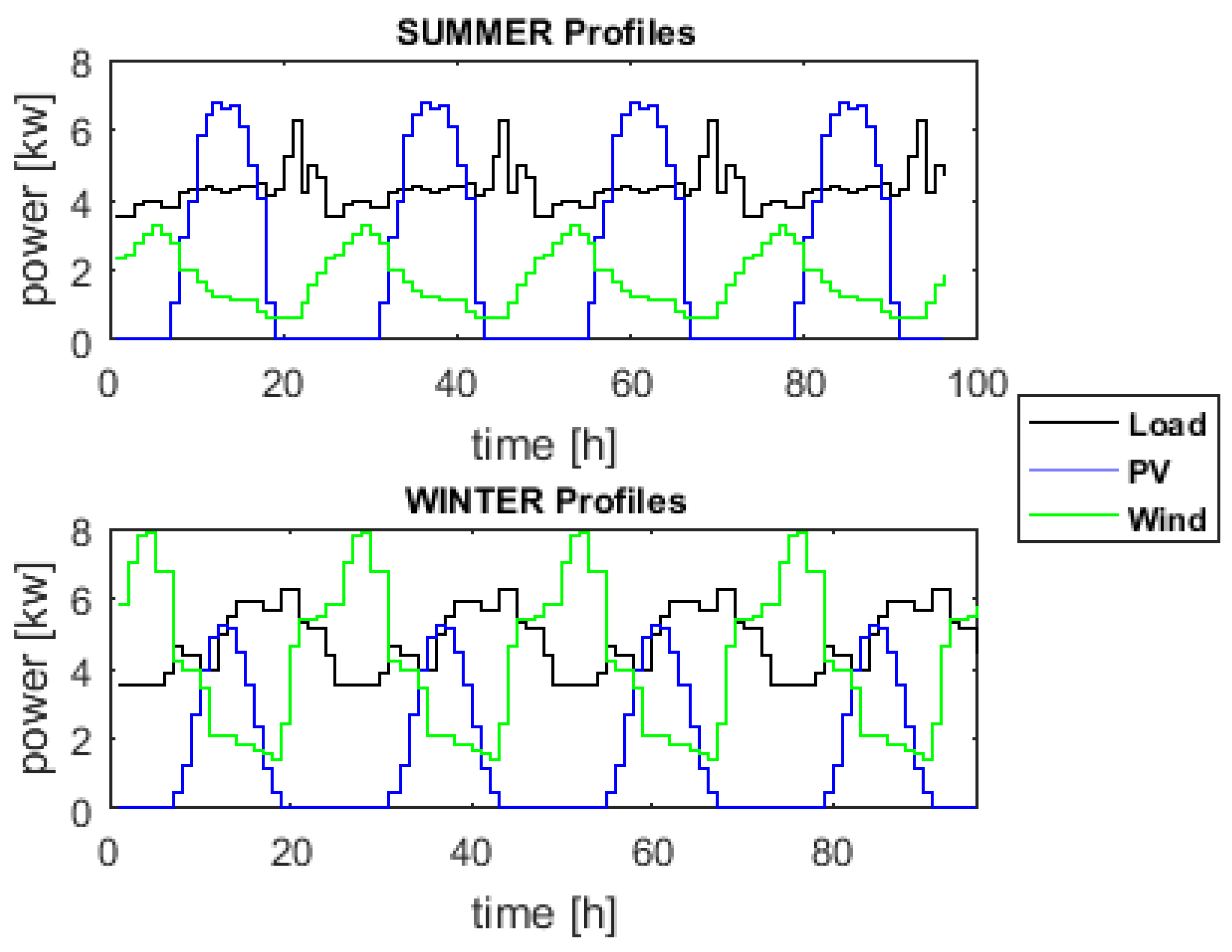
The simulations were made for 96 h (4 days). Some expected profiles of the PV and wind generator, as well as load demands are depicted in Figure 2. In Figure 3, the additive uncertain load demands are represented with the shadowed green area. The state of charge of the batteries and the subsystems’ Initial values are set to ${[20\mathrm{kWh},20\mathrm{kWh}]}^t$. Model parameters and energy prices are summarized in

Table 1. System and control parameter values.

Model Parameters		Energy Prices (e.u)
${\eta }_{bc}$	0.90	Lead-acid battery charging:	0.34
${\eta }_{bd}$	1	Lead-acid battery discharging:	0.34
${\eta }_{hc}$	0.90	Hydrogen battery charging:	0.34
${\eta }_{hd}$	1.0	Hydrogen battery discharging:	0.34
${\delta }^{\min }$	${[10,10]}^t$	Power flow between node:	0.34
${\delta }^{\max }$	${[24,24]}^t$	External grid selling:	4.3
$H_p$	24	External grid buying:	4.3
${\lambda }_1$	2500	Diesel:	8.9
${\lambda }_2^{-}={\lambda }_2^{+}$	12	Hydroelectric:	1.95
${\lambda }_3$	0.1	Wind:	3.7
		Solar:	3.1

.

The profile of a generator represents the maximum power that can be ideally produced by the generator.

5.3. Results

The two proposed robust economic MPC strategies the Open-loop and Closed-loop approaches as well as the nominal approach (i.e., neglecting uncertain demands) have been implemented with YALMIP [14,32] using CPLEX solver in the Matlab environment. The local contol law K defined in (43) for the Robust Closed-loop approach is computed using the LQR method as proposed in [33] obtaining

$$\begin{array}{c}K=\left(\begin{array}{ccccccccc}0.0667& 0& 0& 0& 0& 0& 0& 0& 0\\ 0& 0.0667& 0& 0& 0& 0& 0& 0& 0\end{array}\right)\hfill \end{array}$$

(68)

Two different Cases have been taken into account in the simulations: Case 1 (low and medium demand uncertainty) and Case 2 (high demand uncertainty). Demand uncertainty bounds $\Delta {\theta }_1=\Delta {\theta }_2=$ 0.4 kW and $\Delta {\theta }_1=\Delta {\theta }_2=$ 0.7 kW were considered in Case 1 and Case 2 respectively.

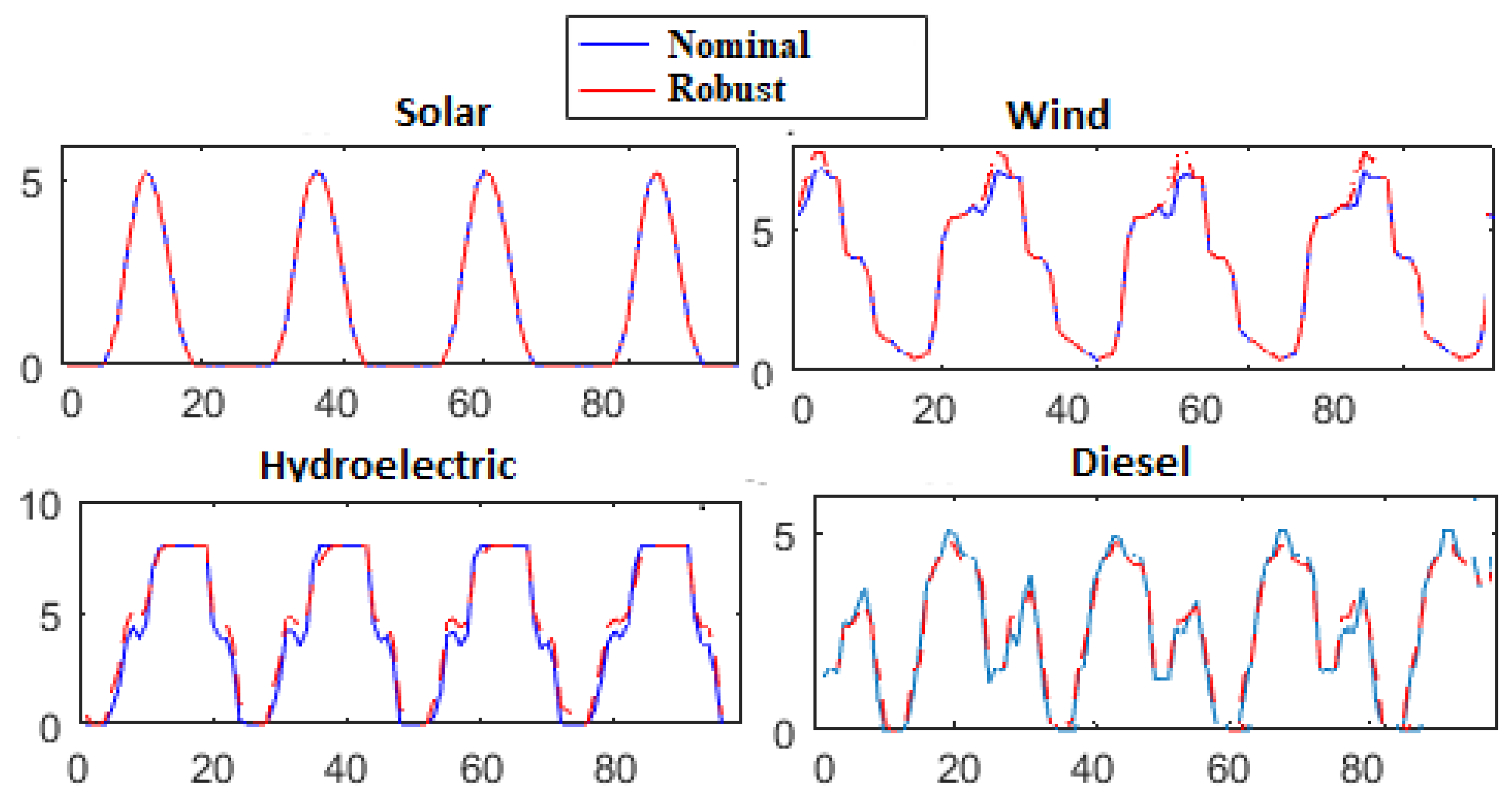
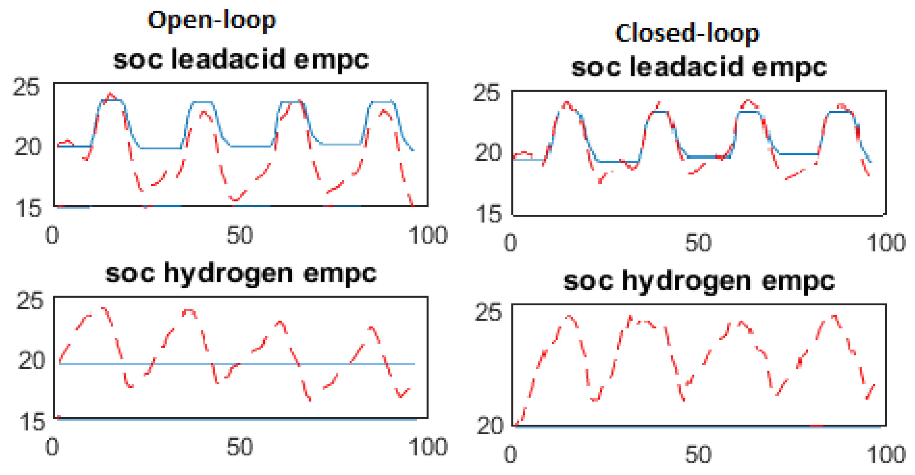
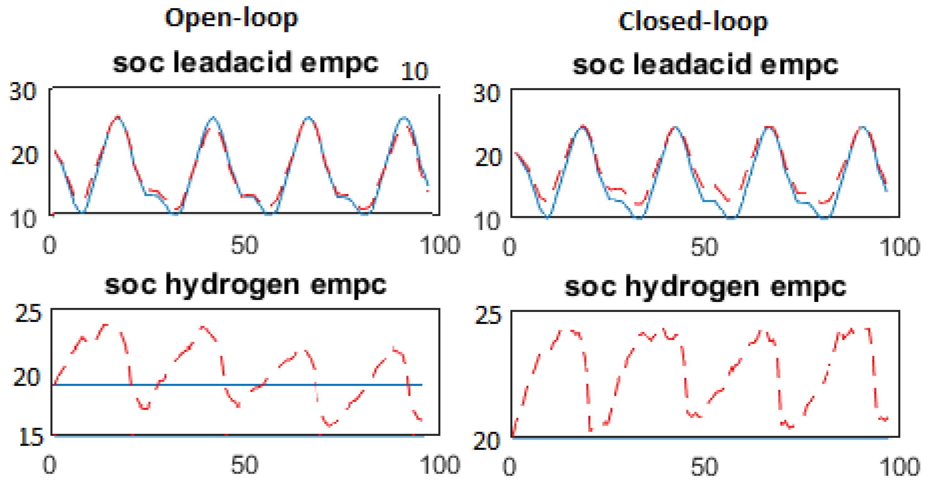
As a general summary of the results depicted in Figure 4, Figure 5, Figure 6, Figure 7 and Figure 8, the diesel and hydroelectric generators delivered between 1 and 1.3 kWh in summer during the first six hours of the day, and in winter in the afternoon for six hours. The batteries delivered between 1 and 2 kWh during the first two hours of the day. 1 kWh was bought from the external grid during the second hour of the day.

Table 2. Daily economic costs Case study 1.

	Nominal EMPC (Zero Uncertainty)	Robust Closed-Loop EMPC	Robust Open-Loop EMPC
Summer	1125.2	1154.4	1143.6
Winter	1428.7	1448.4	1437.1

and

Table 3. Daily economic costs.

	Nominal EMPC (Zero Uncertainty)	Robust Closed-Loop EMPC	Robust Open-Loop EMPC
Summer	1131.7	1184.0	unfeasible
Winter	1433.6	1466.2	unfeasible

show an economic comparison between the two proposed robust approaches and the nominal approach. The overall energy production costs are higher in the robust approaches than in the nominal approach, due to the demand uncertainty. However, the proposed robust methods provide robustness against unexpected changes in the demands.

Robust Open-loop approach is more efficient in economic terms than Robust Closed-loop approach for low and medium uncertainties, as can be seen in Table 2. However, as the demand uncertainty increases, the performance of the Open-loop approach deteriorates, and at some points the problem becomes even unfeasible. This fact can be observed in the results of Case study 2 in Table 3. With high demand uncertainty of 0.7 kW the Open-loop approach becomes unfeasible, while the Closed-loop approach does not present feasibility problems.

The superiority of the Robust Closed-loop approach to its Open-loop counterpart in dealing with high demand uncertainties is due to the fact that, a part of the range of independent variables (37) is devoted to compensate the accumulative effect of demand uncertainties in uncertain state estimation (27). This compensation leads to smaller uncertain state estimation bounds (39) in the Closed-loop approach than in the Open-loop approach. This fact is emphasized in Figure 9 where the evolution of the bounds of state $x_1$ (SOC of lead acid battery) regarding time prediction i. I.e., $x_1^{max}-\Delta x\left(i\right|k)$ and $x_1^{min}+\Delta x\left(i\right|k)$ considering both robust approaches in Case Study 2 (high demand uncertainty) is depicted. As it can be noticed from this figure, the degree of freedom in the evolution of predicted state variables is much more limited in the Open-loop approach than in the Closed-loop one.

6. Conclusions

In this paper, we have developed a novel robust economic MPC method for guaranteeing an optimal control of a smart micro-grid considering an unknown but bounded demand uncertainty. The proposed robust economic MPC strategy tightens in real-time the constraints of the control inputs as the uncertainty goes throughout the prediction horizon.

We have shown how the control inputs can be decomposed into independent and dependent components, thereby offering a possibility of two different robust EMPC approaches: a feedforward (Open-loop) approach that tightens only the dependent components, and a feedback (Closed-loop) approach that incorporates a local feedback controller for tightening also the independent components. The dependent components have further been divided into two parts, whereby one of the parts is bounded by a zonotope and is employed to compensate for any deviation of the actual demand from the forecasted one. We have also carried out a comparison between the Open-loop and Closed-loop approaches and prove that the Closed-loop approach is more robust to demand uncertainty than the Open-loop approach. Finally, the results of a case study have demonstrated that the proposed robust EMPC method can be successfully used to tackle demand uncertainty in energy dispatch of electrical smart micro-grids. The next steps for completing this work will be devoted to the development of an automatic approach of successively selecting optimal control inputs for compensating demand deviations. Furthermore, extending the developed method by including uncertainty of energy prices and renewable energies as done in [19] for a min–max robust method will also be considered.

References

1. Grosso, J.M.; Ocampo-Martínez, C.; Puig, V.; Joseph, B. Chance-constrained model predictive control for large-scale Networks. J. Process Control 2014, 24, 504–516. [Google Scholar] [CrossRef] [Green Version]
2. Ocampo-Martínez, C.; Puig, V.; Cembrano, G.; Creus, R.; Minoves, M. Improving water management efficiency by using optimization-based control strategies: The Barcelona case study. Water Sci. Technol. Water Supply 2009, 9, 565–575. [Google Scholar] [CrossRef]
3. Wu, X.; Hu, X.; Moura, S.; Yin, X.; Pickert, V. Stochastic control of smart home energy management with plug-in electric vehicle battery energy storage and photovoltaic array. J. Power Sources 2016, 333, 203–212. [Google Scholar] [CrossRef] [Green Version]
4. Wu, X.; Hu, X.; Teng, Y.; Qian, S.; Cheng, R. Optimal integration of a hybrid solar-battery power source into smart home nanogrid with plug-in electric vehicle. J. Power Sources 2017, 363, 277–283. [Google Scholar] [CrossRef] [Green Version]
5. Maciejowski, M.J. Predictive Control with Constraints; Prentice Hall: Upper Saddle River, NJ, USA, 2002. [Google Scholar]
6. Wang, L. Model Predictive Control System Design and Implementation Using MATLAB; Springer: Berlin/Heidelberg, Germany, 2009. [Google Scholar]
7. Åström, K.J. Control System Design; University of California Santa Barbara: Santa Barbara, CA, USA, 2002. [Google Scholar]
8. Qi, W.; Liu, J.; Christofides, P. Supervisory Predictive Control of an Integrated Wind/Solar Energy Generation and Water Desalination System. In Proceedings of the 9th International Symposium on Dynamics and Control of Process Systems, Leuven, Belgium, 5–7 July 2010. [Google Scholar]
9. Halvgaard, R. Model Predictive Control for Smart Energy Systems. Ph.D. Thesis, DTU Denmark, Lyngby, Denmark, 2014. [Google Scholar]
10. Prodan, I.; Zio, E. A model predictive control framework for reliable microgrid energy management. Electr. Power Energy Syst. 2014, 61, 399–409. [Google Scholar] [CrossRef]
11. Abate, A.; El Ghaoui, L. Robust model predictive control through adjustable variables: An application to path planning. In Proceedings of the 2004 43rd IEEE Conference on Decision and Control (CDC) (IEEE Cat. No. 04CH37601), Nassau, Bahamas, 14–17 December 2004; Volume 3, pp. 2485–2490. [Google Scholar]
12. Bemporad, A.; Morari, M. Robust model predictive control: A survey. In Robustness in Identification and Control; Springer: Berlin/Heidelberg, Germany, 1999; pp. 207–226. [Google Scholar]
13. Ben-Tal, A.; Goryashko, A.; Guslitzer, E.; Nemirovski, A. Adjustable robust solutions of uncertain linear programs. Math. Program. 2004, 99, 351–376. [Google Scholar] [CrossRef]
14. Löfberg, J. Automatic robust convex programming. Optim. Methods Softw. 2012, 27, 115–129. [Google Scholar] [CrossRef] [Green Version]
15. Zhu, B.; Tazvinga, H.; Xia, X. Switched Model Predictive Control for Energy Dispatching of a Photovoltaic-DieselBattery Hybrid Power System. IEEE Trans. Control Syst. Technol. 2015, 23, 1229–1236. [Google Scholar] [CrossRef] [Green Version]
16. Pereira, M.; Limon, D.; Alamo, T.; Valverde, L. Application of Periodic Economic MPC to a Grid-Connected Micro-grid. IFAC-PapersOnLine 2015, 48, 513–518. [Google Scholar] [CrossRef]
17. Puig, V.; Costa, R.; Sampietro, L. Economic MPC for the Energy Management of Hybrid Vehicles including Fuel Cells and Supercapacitors. In Proceedings of the 2016 UKACC 11th International Conference on Control (CONTROL), Belfast, UK, 31 August–2 September 2016. [Google Scholar]
18. Nassourou, M.; Puig, V.; Blesa, J. Robust optimization based energy dispatch in smart grids considering demand uncertainty. J. Phys. Conf. Ser. 2017, 783, 012033. [Google Scholar] [CrossRef]
19. Nassourou, M.; Puig, V.; Blesa, J. Robust optimization based energy dispatch in smart grids considering simultaneously multiple uncertainties: Load demands and energy prices. IFAC-PapersOnLine 2017, 50, 6755–6760. [Google Scholar] [CrossRef]
20. Ben-Tal, A.; Nemirovski, A. Robust convex optimization. Math. Oper. Res. 1998, 23, 769–805. [Google Scholar] [CrossRef]
21. Vandenberghe, L.; Boyd, S. Semidefinite programming. SIAM Rev. 1996, 38, 49–95. [Google Scholar] [CrossRef] [Green Version]
22. Rawlings, J.B.; Mayne, D.Q. Model Predictive Control: Theory and Design; Nob Hill Publishing: Madison, WI, USA, 2009. [Google Scholar]
23. Ellis, M.; Durand, H.; Christofides, P.D. A tutorial review of economic model predictive control methods. J. Process Control 2012, 24, 1156–1178. [Google Scholar] [CrossRef]
24. Scokaert, P.O.M.; Mayne, D.Q. min–max Feedback Model Predictive Control for Constrained Linear Systems. IEEE Trans. Autom. Control 2012, 43, 1136–1142. [Google Scholar] [CrossRef]
25. Nassourou, M.; Blesa, J.; Puig, V. Robust Economic Model Predictive Control for Energy Dispatch in Smart Micro-grids Considering Demand Uncertainty. In Proceedings of the 24th IEEE Conference on Emerging Technologies and Factory Automation, Zaragoza, Spain, 10–13 September 2019. [Google Scholar]
26. Grosso, J. On model predictive control for economic and robust operation of generalised flow-based networks. Ph.D. Thesis, UPC, Barcelona, Spain, 2014. [Google Scholar]
27. Blesa, J.; Puig, V.; Saludes, J. Identification for passive robust fault detection using zonotope-based set-membership approaches. Int. J. Adapt. Control Signal Process. 2011, 25, 788–812. [Google Scholar] [CrossRef]
28. Blesa, J.; Puig, V.; Saludes, J. Robust identification and fault diagnosis based on uncertain multiple input–multiple output linear parameter varying parity equations and zonotopes. J. Process Control 2012, 22, 1890–1912. [Google Scholar] [CrossRef] [Green Version]
29. Montes de Oca, S.; Puig, V.; Blesa, J. Robust fault detection based on adaptive threshold generation using interval LPV observers. Int. J. Adapt. Control Signal Process. 2012, 26, 258–283. [Google Scholar] [CrossRef] [Green Version]
30. Blesa, J.; Puig, V.; Saludes, J.; Fernández-Cantí, R.M. Set-membership parity space approach for fault detection in linear uncertain dynamic systems. Int. J. Adapt. Control Signal Process. 2016, 30, 186–205. [Google Scholar] [CrossRef] [Green Version]
31. Jaulin, L.; Kieffer, M.; Didrit, O.; Walter, E. Interval analysis. In Applied Interval Analysis; Springer: Berlin/Heidelberg, Germany, 2001; pp. 11–43. [Google Scholar]
32. Löfberg, J. YALMIP: A Toolbox for Modeling and Optimization in MATLAB. In Proceedings of the 2004 IEEE International Conference on Robotics and Automation (IEEE Cat. No.04CH37508), New Orleans, LA, USA, 2–4 September 2004. [Google Scholar]
33. Wang, Y.; Muñoz de la Peña, D.; Puig, V.; Cembrano, G. Robust economic model predictive control based on a periodicity constraint. Int. J. Robust Nonlinear Control 2019, 29, 3296–3310. [Google Scholar] [CrossRef] [Green Version]
Figure 1. Block diagram of the smart micro-grid.
Energies 13 00696 g001
Figure 2. Forecasted profiles of PV and wind generators, and load demands.
Energies 13 00696 g002
Figure 3. Load demands profiles.
Energies 13 00696 g003
Figure 4. Sample winter plots of energy production.
Energies 13 00696 g004
Figure 5. Sample summer plots of energy production.
Energies 13 00696 g005
Figure 6. Sample winter plots of batteries’ State of Charge.
Energies 13 00696 g006
Figure 7. Sample summer plots of batteries’ State of Charge.
Energies 13 00696 g007
Figure 8. Sample plots of batteries’ State of Charge.
Energies 13 00696 g008
Figure 9. SOC bounds of leadacid battery.
Energies 13 00696 g009