Article

On the Way to a Sustainable European Energy System: Setting Up an Integrated Assessment Toolbox with TIMES PanEU as the Key Component

Institute of Energy Economics and Rational Energy Use, University of Stuttgart, Heßbrühlstraße 49A, 70565 Stuttgart, Germany
*
Authors to whom correspondence should be addressed.
Energies 2020, 13(3), 707; https://doi.org/10.3390/en13030707
Submission received: 27 December 2019 / Revised: 21 January 2020 / Accepted: 3 February 2020 / Published: 6 February 2020
(This article belongs to the Special Issue Model Coupling and Energy Systems)

Abstract

:
The required decarbonization of the energy system is a complex task, with ambitious targets under the Paris Agreement, and related policy analysis should consider possible impacts on the economy and society. By coupling the energy system model TIMES PanEU with the impact assessment model EcoSense and the computable general equilibrium model NEWAGE, we present an integrated assessment toolbox for the European energy system capable of internalizing health damage costs of air pollution while simultaneously accounting for demand changes in energy services caused by economic feedback loops. The effects of each coupling step are investigated in a scenario analysis. Additionally, CO2 decomposition analysis is applied to identify the main drivers to decarbonize the energy system. Our results show that integrating externalities forces the system to take early action, which provides benefits on the societal level. Including macro-economic variables has a negative effect on energy service demands and generally reduces the need for structural change, which are still the main drivers of decarbonization. The tighter the models are coupled, the fewer the iterations needed and the lower the CO2 prices resulting from the carbon cap and trade system. In this aspect, an integrated view can provide valuable insights to determine efficient and effective decarbonization paths.

1. Introduction

1.1. Motivation

In order to meet the Paris Agreement targets and limit global warming accordingly, the European Union (EU) must reduce its greenhouse gas (GHG) emissions by at least 80% in 2050 compared to 1990 levels or even achieve carbon-neutrality as also outlined in its “Clean Planet for All” strategy [1]. The required energy transition, which implies deep fuel shifts and significant investments in new technologies, is likely to have impacts on economies since economic growth and energy supply are closely linked, usually resulting in an increased per capita energy and carbon intensity [2]. Depending on the chosen path, the EU energy transition will also affect society and the environment in different ways. Similarly, societal decisions in other policy areas, especially when dealing with other environmental issues than climate change mitigation, may affect the EU energy transition. As, for example, both climate change mitigation and air pollution control require changes in the energy system, they may hamper or foster each other to achieve their goals [3].
Therefore, the EU energy transition should be analyzed by also taking into account different dimensions such as the economy and the environment which also affect the decision-making processes in the energy system. To this end, different integrated assessment models (IAM), for both EU and non-EU regions, have been developed and applied in recent years to analyze different transition pathways, identify relevant decarbonization drivers and understand their impacts on the energy system as well as possible effects on the economy and society. Before introducing the Integrated Assessment Toolbox developed and applied in this study, a review of previous work in this field is presented first.

1.2. Background

The need for an integrated assessment framework to study energy transitions has been widely recognized in recent literature. Integrated assessment models or frameworks combine expertise from different disciplines and are often applied to identify, study and assess climate change impacts, key challenges and respective mitigation strategies (A good overview of Integrated Assessment Frameworks in the field of climate change mitigation is given in a “Carbon Brief” Q and A: https://www.carbonbrief.org/qa-how-integrated-assessment-models-are-used-to-study-climate-change (last checked: 15-12-2019)). Their main purpose is to provide insights into how, based on constructed scenarios, human behavior, development and societal choices affect different systems and the natural world. In particular, integrated assessment models are also applied in the Intergovernmental Panel for Climate Change (IPCC)assessment reports to identify and discuss possible impacts on and interactions between economic and social developments, technical system and natural environments of different emission scenarios. In these world-wide studies, six different integrated assessment models are applied, covering different spatial areas, representing different modelling approaches and partially focusing on different aspects [4]. In this review, we focus on other integrated assessment models applied outside the IPCC studies, which have an energy system model at their core.
The link between an energy system model and macroeconomic model, for example, has been established in the MESSAGE-MACRO model [5]. The corresponding study focused on the factors which affect the energy supply costs calculated in the energy system model by feeding these costs to the macroeconomic model to create consistency between the energy demand and supply curves. For two different scenarios, the gross domestic product (GDP), energy supply and demand, and energy prices were compared after the link was established.
In another study, the techno-economic TIAM-WORLD model has been linked with the general equilibrium model GEMINI-E3 together with a climate model, PLASIM-ENTS, to specifically discuss the impacts of climate change on the energy system with an emphasis on heating and cooling demand [6]. The results of this study showed that the link between these three models shows a different picture in terms of required investments in generation capacity at the regional level than the energy system model on its own. This, in turn, results in increased energy prices, especially due to rising cooling demand because of increasing average temperatures. It is observed that the welfare gains and losses are affected by changes in energy exports and imports. However, the changes in the heating and cooling demands do not have a significant impact on economic parameters such as GDP.
Studies with links between energy system and impact assessment models can be found in literature as well. In [7], the methodology to internalize life-cycle data and external costs in a TIMES model is presented. According to this link, the unit health damage costs caused by the pollutants are calculated exogenously and they are fed back to the energy system model. The synergy between the environmental taxes on pollutants and different CO2 mitigation scenarios in Italy are discussed in detail in [8]. Similar analyses are also delivered at the EU level to see the impact of externalities in the energy system [3]. Their results indicate that internalizing the externalities in a decarbonized energy system induces welfare savings by further reducing air pollution. The energy system is still able to achieve the given GHG reduction targets with lower utilization of biomass and conventional carbon capture and storage (CCS) technologies due to associated health impacts.
Aside from integrated assessment models, CO2 decomposition analysis is usually applied in different parts of the energy system to identify the main drivers for decarbonization and their impact on the energy transition, including economic effects reflected in activity and demand changes. In [9], a methodology has been proposed to generate marginal abatement cost curves based on the results from an energy system model and a decomposition analysis of CO2 reductions. Four categories represent the relevant effects in emission reductions: demand changes (activity effect), technology switches (structure effect), efficiency improvements (fuel intensity effect), and reduction in the carbon intensity of secondary energy carriers (carbon intensity effect). For the decomposition analysis, the log mean divisia index (LMDI) has been chosen as the preferred method. In the study the focus was on the transport sector decarbonization in the UK and, according to their findings, structural shifts and reduced carbon intensity of fuels are responsible for the majority of emission reductions. On the other hand, demand reduction, which is assessed by considering elastic demand functions in the model, shows only a minor but constant contribution to CO2 reductions in transport. In another study, the relative effects of different factors on the changes in CO2 emissions have been analyzed for the Turkish manufacturing industry between 1995–2001 [10]. Again, LMDI has been applied as a decomposition method with energy intensity and economic activity being identified as the main drivers. LMDI was also used in [11], with a focus on the Iranian energy market between 2003–2014. Industrial energy consumption, the carbon intensity of electricity generation and carbon emission due to total (fossil) fuel consumption, are investigated as drivers. They concluded that increased consumption was the main reason for increases in Iran’s CO2 emissions.

1.3. Research Question

According to the available literature and based on our best knowledge, so far, an energy system model is either linked to an environmental impact assessment or a macro-economic model and only impacts from a single link are discussed. Consequently, as we aim to fill this gap, the integrated assessment toolbox developed in this research brings all of these three elements together and considers the technical, economic and environmental dimensions simultaneously in the energy transition analysis on the EU level. Through a comparative and qualitative scenario analysis, the toolbox aims to provide new policy insights regarding economic impacts of decarbonization, their relation with and effect on the energy system as well as potential trade-offs between energy system transitions and related externalities. This study introduces an additional novelty by applying a CO2 decomposition analysis to assess the impact that each model coupling has on the decarbonization path.

2. Methods

In this section, the models applied in the study are introduced first. Next, the methodology for the links between the models is described and the process to create the Integrated Assessment Toolbox is presented. In the following sections, we present a methodology to assess the impacts of linking the models on the CO2 decomposition, as this is one of the aims of the study. Finally, the section is concluded with the description of the scenarios applied to identify the impacts of the links in the EU energy transition.

2.1. Models Applied

In this section, we introduce the three models applied in our study—TIMES PanEU, EcoSense and NEWAGE—which provide the foundation for the Integrated Assessment Toolbox as depicted in Figure 1.
As an energy system model, TIMES PanEU is employed. The model generator TIMES has already been employed in multiple studies proving its compatibility to provide similar analyses, as shown for example in [12,13]. In particular, TIMES PanEU also fulfills the most relevant requirements such as sectoral integration, covering the entire energy system as well as the potential of the domestic sources such as biomass. As it also includes all the member states, it can also provide policy-relevant insights not only at the EU level but also at the national level. EcoSense is chosen as a health impact assessment model in our study. EcoSense is a reference implementation of the Extern-E methodology, which forms the foundation of externality assessment in the field of energy. As such, EcoSense is considered to be best fitting for the Integrated Assessment Toolbox. NEWAGE is applied as a general equilibrium to have the macro-economic insights through the energy transition. NEWAGE has a detailed electricity sector modeled which is quite crucial in areas such as a coupling process. Additionally, considering the sectoral disaggregation in TIMES PanEU and NEWAGE, the sectors in NEWAGE can reflect the development in all the end-user sectors in TIMES PanEU.

2.1.1. Energy System Model: TIMES PanEU

TIMES PanEU is employed as an energy system optimization model to be further linked to EcoSense and NEWAGE in our study.
TIMES PanEU is built with the TIMES model generator, in the modelling environment GAMS. It is a model generator to create bottom-up energy system models with linear programming. It has been developed and maintained within the Energy Technology System Analyses Program (ETSAP) by the International Energy Agency (IEA) [14]. The data management system (VEDA-TIMES) creates an energy system model [15]. Through this data system, the input data, the structure of the model and all the scenario-related information are given to the model and they are converted to mathematical equations. The model aims to minimize the total discounted system cost in a given timeframe to meet exogenously given service demands [16] with a perfect foresight principle. TIMES PanEU covers the European Union countries as well as Norway and Switzerland and each country represents a single region in the model. The modelling horizon spans from 2010 to 2050, split into 5 year-time steps. A year is divided into 12 time-slices, 4-seasonal and 3-day levels (day, peak and night). Greenhouse gas emissions (CO2, CH4, N2O) and other pollutants (SO2, NOx, CO, NMVOC, PM2.5, PM10) are included in the model. The basic structure of the model is called reference energy system (RES). RES includes all relevant energy, material, and emission flows from the primary production to meet the demand of energy services for each region defined in the model [17]. RES of the model covers the entire energy system, from the supply of resources to the service demand. Different technologies are modelled to make the interactions possible between the parts of the energy system. Primary energy sources are modelled according to country potentials and the trade possibilities from the neighboring countries. Different cost potential curves are defined for each of the sources such as crude oil, natural gas, coal, lignite, etc. The World Energy Outlook 2016 prices [18] and average country mining costs are taken as a reference to determine the cost figures. Various bioenergy carriers are included by taking into account the country’s potential and their costs. No constraints are considered for biomass trade within the EU regions. Land availability for biomass cultivation is given in the model based on [19]. Additionally, other conversion technologies such as refineries, gasification and power-to-gas are part of the model [14].
In the electricity sector, the electricity supply at different voltage levels is modelled through different technologies. The technologies are classified according to the input fuels and technology type and they are aggregated by power plant type. New technologies such as electricity storage, hydrogen technologies and CCS technologies are modelled as investment options during the time horizon. The availability of certain technologies such as CCS is determined according to the expected schedule of technologies to be commercially available in the market [20]. Cogeneration plants (CHP) for centrally supplied district heating are given as a choice in the model to provide both electricity and heat. Power-to-heat technologies together with heat storages are applied in the public heat supply. Capacities deployed, generations, energy prices, energy flows as well as emissions are calculated based on given input parameters to the model.
The industrial sector is divided into energy-intensive and non energy-intensive industries. The energy-intensive industries cover the categories iron and steel, aluminum, copper, ammonia, chlorine, cement, lime, flat glass, and paper; whereas the non energy-intensive industries include other non-ferrous metals, other chemicals, other non-metallic minerals, food and tobacco and other industries. Industrial auto producers are also modelled [21].
In the household, commercial and agriculture segment, the energy service demands are disaggregated according to different sectors. Various technologies, aggregated according to technology type and energy carrier, are implemented to provide the energy service demands. The process to supply the agriculture demand is defined as one general process. The underlying assumptions of the existing demand figures in TIMES PanEU are consistent with the socio-demographic assumptions of the EU reference scenario [22].
The transport sector is disaggregated according to transportation mode: car, bus, motorcycle, passenger train, freight, air traffic (external and internal) and navigation categories. The passenger transport is modelled in the unit of passenger-km (Pkm). The freight is modelled in ton-km (Tkm). Different vehicles technologies based on the different energy carriers are modelled for each demand category mentioned above. Hybrid technologies are available. Technologies deployed together with the emissions that they produce and the energy flows are calculated in this sector as well. Mitigation options are also modelled to decarbonize the aviation and navigation sectors according to given milestones for the technologies in [23].

2.1.2. Health Impact Assessment Model: EcoSense

The impact assessment model EcoSense is applied to simulate and estimate health impacts due to air pollution across Europe. By following the impact pathway approach, as developed in the ExternE project series [24], EcoSense is designed to provide cost-benefit analysis of different air pollution mitigation scenarios up until 2050.
The impact pathway approach, as implemented in EcoSense, links changes in national emissions of the main air pollutants (SO2, NOX, NMVOC, NH3, PM10 and PM2.5) to health impacts across Europe. For this purpose, an atmospheric dispersion model is integrated with epidemiological studies and an economic assessment of impacts [25,26]. In a first step, a parameterized version of the EMEP/MSC-W model [27,28] is applied to estimates changes in concentration levels of Ozone, NO2 and particulate matter (PM2.5 and PM10, incl. primary and secondary particles) attributable to changes in national emissions on a 0.5° × 0.25° grid covering Europe and neighboring regions in Africa and Asia. Based on concentration-response functions recommended by the World Health Organization (WHO) [29], stating the change in relative risk of a specific outcome (inter alia increased mortality, hospital admissions and workdays lost) due to an increase in exposure to air pollution, additional cases related to the original changes in emissions are then estimated by also considering detailed population data and background disease rates [30]. The population data in EcoSense considers the spatial distribution of the high-resolution population density grid for Europe [31] as well as country-specific age structures and population projections based on UN data. Finally, the different health impacts are aggregated in monetary values by applying a willingness-to-pay approach for impacts on mortality (“Value of Life Year”) and standard prices for all other impacts. EcoSense applies monetary values based on the HEIMTSA/INTARESE case study [26] with gaps filled by considering values from [30]. By relating the absolute costs of an emission scenario to the respective amount of emissions, unit cost factors can also be estimated. This application is described in more detail in [3] and [32].

2.1.3. General Equilibrium Model: NEWAGE

In this work we utilize the global computable general equilibrium (CGE)model NEWAGE (National European World Applied General Equilibrium, for more details about the NEWAGE model, visit https://www.ier.uni-stuttgart.de/forschung/modelle/NEWAGE/), to identify policy impacts in the economy. In this model, the world is divided into 18 regions, as shown in Figure A1, and production is split into 18 sectors, listed in Table A1. Additionally, the model considers that each region has a representative agent with endowments of four primary factors of production, namely capital, labor, natural resources and CO2 certificates. Labor market is imperfect and heterogeneous, being divided into highly qualified (skilled) and less-qualified (unskilled) labor. Finally, the model is recursive-dynamic and uses Cobb–Douglas, Leontief and constant elasticity of substitution (CES) to represent production and utility possibilities, as shown in Figure A2, and are based on [33] and [34].
NEWAGE also has a detailed representation of the electricity-generation system, with 18 production possibilities described as combinations of technology and load categories, namely base, mid and peak, as shown in Figure A3. In this case, some technologies are considered to be used in every load category, such as gas, while others are used in only one or two load categories, such as wind and solar are used only in mid-load.
The framework of NEWAGE enables the analysis of impacts of different political interventions on macro-economic indicators, such as GDP growth, sectoral gross value added (GVA), employment and competitiveness. Specifically, for the coupling procedure, we also calculate regional net income, calculated as the sum of income from capital and labor minus payments of taxes to the government, and regional utility, defined as the total consumption by households.

2.2. Integrated Assessment Toolbox

In this section, the links between the energy system model, TIMES PanEU, the health impact assessment model, EcoSense, and the general equilibrium model, NEWAGE are presented. The three models are coupled with TIMES PanEU at the core; the respective data exchange and links are shown in Figure 2.

2.2.1. Linking Energy System Model with Health Impact Assessment Model

We developed a link between the TIMES PanEU energy system model and the health impact assessment model EcoSense to analyze the interaction between GHG mitigation and air pollution and to assess the health impacts from energy-related emissions. The impacts of such a link on the energy transition have already been analyzed in different studies [3,8]. The link itself is depicted in the upper part of Figure 2, together with the relevant data exchange.
In a first step, common assumptions of both models, such as population growth and general socio-economic developments are harmonized. Most importantly, the time horizon, milestone years and monetary base year are matched. Similarly, the different sectors in TIMES PanEU are matched to specific emission source categories in EcoSense, differentiating different release heights as well as mobile and stationary source (Since we only consider country specific damage costs in this study without any sectoral differentiation, this match was actually not necessary). As a following step, the existing emission coefficients (kt/PJ) of air pollutants (SO2, NOx, CO, NMVOC, PM2.5, PM10) are updated in TIMES PanEU to reflect the latest developments and emission standards induced by the Clean Air Policy Package [35]. The coefficients are disaggregated according to sectors, regions, technology and fuel types [32]. Based on these coefficients, TIMES PanEU provides to EcoSense sector- and country-specific total emissions (kt) for each pollutant. By utilizing the data from TIMES PanEU, EcoSense calculates unit health damage costs (€/kg). These are disaggregated according to different pollutants without sectoral decomposition and fed back to TIMES PanEU.
The unit health damage costs are implemented as an additional parameter and the total health damage costs are calculated in the model according to the following equations [36]:
DAM (EM) = α * EM (β + 1)
where:
EM (kt) is the emission in the current period,
DAM (EUR/kt) is the health damage cost in the current period,
β ≥ 0 is the elasticity of the marginal health damage cost to amount of emissions,
α > 0 is a calibrating parameter, which may be obtained from dose-response studies that allow the computation of the marginal health damage cost per unit of emission at some reference level of emissions.
If the marginal cost at the reference level is denoted with MC0, the following holds:
MC0 = α * (β + 1) * EM0 (β)
which is what is calculated by EcoSense according to the link between the models.
When there is no elasticity factor assumed (β = 0), i.e. when there is a linear relationship between health damage costs and amount of emissions, the first equation can be simplified as follows:
DAM (EM) = (MC0 * EM0) * EM
The cost figures (MC0) are calculated for each region in TIMES PanEU according to milestone years. The range of cost figures according to countries and sector disaggregation is available in [32].
The health damage costs can be used for two types of assessments in energy system modelling:
  • To provide an exogenous economic evaluation of the health damage by the energy system, without any feedback to the cost-optimization function (ex-post);
  • To study how the optimal energy supply mix would change, if health damage costs were to be internalized, as part of the cost-optimization function (ex-ante). This would correspond to a scenario in which the health damage costs of air pollutants are considered in the energy system design.
Both types of assessment are carried out as a part of our study and insights are given in Section 3. An iteration between TIMES PanEU and EcoSense is not required for the conducted scenario analysis as there are not any feedbacks to be iterated between the models. Due to the linear relationship between the total health damage costs as calculated by EcoSense and the total emissions, the unit costs are independent of the absolute amount of emissions and climate mitigation policies. This means that the values are scenario-independent as well.

2.2.2. Linking Energy System with General Equilibrium Model

The main objective of the link between TIMES PanEU and NEWAGE is to compensate the limitations of each model through their cooperative work. The structure of NEWAGE, in which production sectors are interconnected, depicts in a transparent manner the variations caused by decarbonization in GDP development and sectoral growth, which modifies the demand for energy services. TIMES PanEU can, in return, use the results from NEWAGE to update its own sectoral demand for energy services. Following this, TIMES PanEU uses its highly detailed depiction of the energy system to provide a more accurate electricity mix back to NEWAGE. The link between the two models is intended to happen after the link between EcoSense and TIMES PanEU to complete the integrated assessment toolbox, where the synergies between air pollution control and energy transition are already taken into account (ex-ante). The data exchange between the two models is presented in the lower part of Figure 2.
Before initiating the iteration process, NEWAGE and TIMES PanEU need to harmonize their socio-economic assumptions. To do so, projections about population and GDP growth are compiled to a common reference scenario (the respective scenario assumptions are explained in Section 2.4), which is implemented in both models together, following the method proposed in [37]. Additionally, NEWAGE is calibrated to the technology development of TIMES PanEU by replicating its sectoral CO2 emissions and electricity mix of the chosen reference scenario. The harmonization and calibration process is supposed to ensure comparability between the results from both models.
The iteration process (Figure 2) begins with TIMES PanEU, as it produces the first results of the electricity-generation mix. Following, NEWAGE is set for the designed scenario and fixes, with a small deviation margin, its electricity generation mix to be at the same level as that from TIMES PanEU. Next, NEWAGE produces results for GDP development, sectoral GVA, net income and utility. Finally, the existing sectoral energy service demands in TIMES PanEU are updated according to Equation (4) and the sectoral match between the models given in Table A3 in Appendix B. As there are feedbacks between the models with the updated energy service demands in TIMES PanEU and electricity mix in NEWAGE, the two models are run iteratively. Although the relation between energy use and economic developments has already been proved in [2], it is also discussed in [38] that energy service demand values are not only affected by the economic developments in a country. There are factors such as population growth, efficiency improvements, energy production and transportation of energy which also influence the energy service demand development. Additionally, the impact of social factors such as comfort, behavior or happiness should also be considered. Therefore, we apply a decoupling factor DF to balance the impact of macro-economic variations and other impacts on the energy service demands, which also reflects a certain degree of demand inelasticity in energy services:
E D s , ( x + 1 ) S C E   =   ( E V i , x S C E E V i R E F ) ( 1 D F ) +   E D s R E F D F
In Equation (4), ED denotes the energy service demands of sector s in iteration x and scenario SCE, while REF denotes the reference scenario. EV designates the level of the economic variable i, which is related to sector s according to Table A3 in Appendix B. As mentioned, DF represents the decoupling factor, which determines the weight that the sectoral energy demands from the reference scenario will have on the updated values. Thus, if a decoupling factor of 25% is applied, it is assumed that 75% of the demand development is reflected by the general economic development, while 25% are mainly influenced by other factors, such as efficiency gains, changing consumption patterns or population.
To summarize, the steps of the iteration process are the following:
  • TIMES PanEU provides the results of the electricity mix calculated for a decarbonization scenario to NEWAGE as shown in Figure 2. The technology match for this step between the models is given in Table A4. in Appendix B.
  • NEWAGE calculates economic variables influencing energy service-demand growth patterns based on the provided results by TIMES PanEU.
  • Energy service-demand projections are updated in TIMES PanEU based on chosen economic variables as calculated by NEWAGE.
  • The convergence criterion is computed.
  • If convergence criterion is not within the range of convergence, go back to step 1.
In this study, we use the relative variation of GDP from NEWAGE between the iterations as the convergence criteria. This choice is based on the fact that GDP is a product of all production sectors and consumption, so it stops varying when other economic variables in NEWAGE reach convergence. A derivation of ± 0.005% is assumed to be sufficiently small to account for convergence.

2.3. Decomposition Analysis

In this study, we apply decomposition analysis to identify relevant decarbonization drivers and understand their impacts on the decarbonization of the energy system with also an explicit focus on the differences resulting from the links with an impact assessment and general equilibrium model. Similar to the other studies reviewed in Section 0 [9,10,11], we also opted for LMDI as the basic method, since this guarantees full decomposition without any residual emissions [10].
CO2 emissions in the overall system are decomposed into four different effects in our study, following a similar approach as in [9]: Activity effect, structure effect, fuel-intensity effect and carbon-intensity effect. The activity effect refers to the changes in CO2 emissions due to variations in energy service demands. In our study, the link with the general equilibrium model NEWAGE affects the energy service demands which enables the model to take into account the macro-economic variations during the energy transition. Structure effects describe emission changes because of the technological switch. The building of a solar power plant to replace the power generated by a decommissioned coal power plant can be given as an example of this effect. The fuel intensity effect defines the difference in CO2 emission due to switching to more efficient technologies without changing the energy carrier. One example of this effect is the replacement of a gasoline car in the transport system with a more efficient gasoline car. Differences from changing the carbon content of fossil fuels are captured by the carbon intensity effect, for example changing an oil boiler with a gas boiler in the residential sector. Based on this decomposition total CO2 emissions in the energy system can be formulated as follows [9]:
CO 2 ,   total   system   = i a c t i v i t y i ( j a c t i v i t y i , j a c t i v i t y i f u e l i , j a c t i v i t y i , j   C O 2 , s y s t e m , i , j f u e l i , j )
Activity is the energy service demand in PJ here and i refers to sector and j to technology in Equation (5). When the equation is rewritten as in Equation (6), where a represents the demand, s does the structure, f does the fuel and c does the carbon content. The changes in CO2 emissions can be also described with Equation (7):
CO 2 ,   total   system = i , j a i s i , j f i , j c i , j
Δ CO2 = Δ demand change + Δ structural shift + Δ efficiency improvements + Δ fossil fuel switching.

2.4. Scenario Structure and Assumptions

To analyze the impacts of different variables through the energy transition, we investigate a scenario with a Europe-wide target to reduce greenhouse gas (GHG) emissions across all sectors and all the member states in EU28 in 2050 by at least 85% compared to 1990 levels. To allow for a continuous reduction over the years, we implement the milestones displayed in Table 1. To achieve these targets in 2050 and ensure a smooth and realistic transition path, additional milestones are set in 2030 and 2040. These milestones are determined according to given targets in [2]. In Table 1, the reduction targets are also given according to the emission level in 2015 as this is the reference year in this study.
The EU reference scenario [22] is used to define the socio-economic assumptions as a basis for the reference scenario utilized in this study. Both models harmonized their relevant assumptions accordingly, including decarbonization targets in TIMES PanEU and GDP development in NEWAGE. Furthermore, technology development in NEWAGE is calibrated to the respective TIMES PanEU results of this reference scenario.
For the link with EcoSense, the health-damage cost factors are introduced into the energy system model starting from 2020 as the base year of the model is 2015 and these costs are not taken into account in the system design in reality. It is also assumed that these costs are phased in gradually, with only half of the actual health-damage costs applied in 2020. This stepwise introduction also matches with the 5-year model structure of TIMES PanEU [3]. From 2030 on, the unit health damage cost (€/kg) values calculated by EcoSense are employed directly in the model.
Aside from the given decarbonization targets for Europe, NEWAGE, as a world model, also needs to make assumptions about decarbonization efforts in the rest of the world. For the reference scenario, an emissions path consistent with the reference technology scenario (RTS) from the Energy Technology Perspectives (ETP) 2017 study [39] was assumed. For the remaining scenarios, the targets are diverse and represent a coalition between regions that want to pursue higher GHG reductions than in the business-as-usual scenario. Detailed targets are described in Table A1.
As the aim is to take into account all the different drivers in the energy system development, TIMES PanEU is first linked with EcoSense. Here two scenarios are defined to address the impacts of having damage costs in TIMES PanEU. In the GHG scenario (Table 2), damage costs are not considered in the optimization function (ex-post). In the GHG_DAM scenario, damage costs are considered in the optimization function (ex-ante) and only this version is finally used in the iterations with NEWAGE as given in Table 2. As there is also no scientific consensus on how much energy service demands are solely influenced by economic development or on how big of a role other socio-economic parameters and developments play, we conduct a sensitivity analysis and apply three different decoupling factors for the link between TIMES PanEU and NEWAGE: 25%, 50% and 75%. These scenarios refer to the integrated assessment toolbox (IAT). Together with the stepwise coupling of the three models, this results in a total of six scenarios, which are also described in Table 2.
The following technical assumptions are applied in the scenario structure in TIMES PanEU across all the scenarios in Table 2:
  • The electric vehicles cost assumptions are developed according to the learning curve approach to calculate the cost of the battery packs in the vehicles. A learning rate of 16% is assumed, according to [40].
  • The decommissioning curves of the existing nuclear power plants are determined based on [41].
  • Energy-efficiency technical measurements in industry are included as an option based on [21].
  • Existing and forthcoming electricity exchange capacities are taken from [41].
  • Livestock emissions are included in all the pathways based on [42].
  • Fuel price assumptions are taken from [18].
  • Heat-saving processes and their potential in residential buildings are included according to [43].
  • Techno-economic assumptions such as investment cost, variable costs, availability factors assumptions for solar PV, wind on-shore and off-shore, tidal and wave energy are in line with [22] for the reference scenario. According to deployment scenarios of these technologies, higher cost reductions might be expected [44]. Therefore, techno economic assumption of these technologies are taken from [44] for the other scenarios structured according to Table 2.

3. Result

In this section, we follow the order of the integrated assessment toolbox building process to discuss our findings. In Section 3.1., we present insights from the internalization of the externalities in the energy system. Impacts of the macro-economic variations with the link through NEWAGE are explained in Section 3.2. In this sub-section, insights gained through the iteration process and the effect of different decoupling factors are discussed in detail as well. We conclude the section with findings from the decomposition analyses for the entire energy system together with the remaining CO2 emissions and sectoral decomposition of transport.

3.1. Impact of Externalities in the Energy System

In the integrated assessment toolbox that is built, air pollutants and their health damage costs are integrated into TIMES PanEU through the link with EcoSense. By comparing the reference, greenhouse gas (GHG) and greenhouse gas damage (GHG_DAM) scenarios, co-benefits and interactions between decarbonizing the energy system and air pollution mitigation can be identified. As there are associated uncertainties especially with the absolute values of damage costs integrated in TIMES PanEU, only relative differences to the reference scenario can be interpreted to provide relevant and meaningful insights from their integration.
Before internalizing the health damage cost in the system in 2020, no significant differences are observed between the Reference and GHG scenarios. However, the GHG reduction target results in better air quality and consequently in savings in health damage costs after 2020 (Figure 3, ΔGHG). In 2030, all cost savings occur mainly in three sectors: supply, electricity and industry. The sector descriptions and their scope are given in Section 2.1.1. Lower utilization of the gasification processes creates the difference in the supply sector. Higher deployment of renewables helps to clean up electricity and industry sectors, not only with regard to GHG but also with regard to air pollutants. Later, savings are also achieved from changes in the residential sectors. As one of the main existing heating technologies, new oil boilers are still deployed in the reference scenario. Although they are characterized by improved efficiency, they still emit high levels of GHG and air pollutants. Hence, they are replaced with cleaner heating technologies such as heat pumps in the GHG scenario, which also further reduces emissions of air pollutants along with the health damage costs. With the internalization of the health damage costs in the optimization function (GHG_DAM), this replacement accelerates; therefore, earlier reductions and cost savings are seen compared to the GHG scenario. Similarly, the introduction of the health damage costs in the optimization function leads to an early coal exit in the residential sector, which results in visible savings already in 2030. Additionally, less biomass utilization and, in turn, a higher rate of other renewables, help to further reduce damage costs associated with air pollution from the residential sectors. Compared to the reference scenario, savings in health damage costs caused by changes in agriculture can be observed in both of the scenarios, though they are more visible when these costs are internalized in the optimization function (GHG_DAM). The savings are mainly the result of utilizing fewer petroleum products. Again, internalizing health damage costs (GHG_DAM) reduces the biomass consumption, not only in residential and agriculture but also in industry and electricity, which results in a slightly higher level of cost reduction in this scenario. A detailed analysis of the related changes in the energy system and the respective levels of air pollution are also given in [3,32].
The impact of internalizing health damage costs can also be seen in the marginal CO2 mitigation cost (Figure 4). Introducing health damage costs to the system (GHG_DAM) brings lower marginal CO2 mitigation costs, especially in the early years. With increasing ambition to reduce GHG emissions over the time horizon, however, the reduction target itself becomes more dominant and the additional benefit of lower marginal CO2 mitigation costs diminishes (2030 difference vs. 2050 difference in Figure 4).
The reductions in externalities achieved, which are reduced GHG emissions and savings in damage costs, are partly compensated for by higher cumulated, discounted system costs, presented as net present value in 2015 (NPV 2015) in Figure 5. Despite these higher systems costs, both the GHG and GHG_DAM scenarios achieve net benefits in social costs compared to the Reference scenario. Increased innovation effort is assumed to occur in the case of GHG mitigation targets, which is reflected by more progressive techno-economic developments and assumptions in the corresponding scenarios as explained in Section 2.4. Therefore, this effort can offset the additional push needed to decarbonize the energy system resulting in almost identical system costs in the GHG and the reference scenario. Regarding the total social costs as the sum of system and health damage costs, the GHG scenario still shows a benefit of 596 bn€ from total social cost through savings in total damage costs compared to the Reference scenario. These are even higher in the GHG_DAM scenario where the health damage costs are internalized, although partly being compensated by increased system costs. Compared to the GHG scenario, internalizing health damage costs of air pollutants still results in additional benefits of 333 bn€ which leads to the lowest social costs between the three scenarios considered.

3.2. Impact of Macro-Economic Variations in the Energy System

In this sub-section, we discuss the impact of macro-economic variations in the energy system with the introduction of a carbon cap and trade system. We begin by presenting the selected indicators and their development from the general equilibrium model to show how the different economic variables are affected by a carbon cap and trade system which reasons the different energy service demands developments in the energy system. In the following sub-section, we provide insights from the iteration process between the energy system model and the general equilibrium model and the impact of applying different decoupling factors. We conclude the section by analyzing the selected indicators from both of the models after the models are converged.

3.2.1. Impact of a Carbon Cap and Trade System on the Economy

Compared to the reference scenario, lower CO2 emission caps are introduced in GHG_DAM scenario after the year 2020. As expected, the lower availability of certificates in the market has significant effects on the economy, as shown in Figure 6. This Figure is produced with results from NEWAGE using the same electricity generation mix as TIMES PanEU for this scenario, but before starting the iteration process. GDP levels are lower in GHG_DAM, compared to the reference scenario, by 1.5% in 2030 and 3.2% in 2050. On the other hand, the gap between the two scenarios in net income is decreasing with time, from −1.4% in 2030 to −0.7% in 2050, as the revenues from emission certificates are paid back to the consumers in the form of a lump sum.
Regarding industrial production, we show the GVA variations of the chemical and iron and steel industries as they are energy-intensive sectors with a high consumption of fossil fuels. This makes them more vulnerable to the scarcity of emission allowances. In Figure 6, it can be seen that the impact of the emission targets on these sectors is higher than the impact on GDP development. GVA of the chemical industry in GHG_DAM is 3.4% lower than the reference scenario in 2030 and 8.3% lower in 2050. Additionally, GVA of iron and steel in GHG_DAM is 0.3% lower in 2030 and 12% lower in 2050, compared to the reference scenario.
The last economic variable displayed in Figure 6, is the GVA of the Transportation sector, which includes transportation of goods and passengers (without private individual transportation) by land, air and water. In the GHG_DAM scenario, this sector has a GVA level 0.8% higher than the reference scenario in 2030, because the energy-intensive sectors consume less fossil fuels which makes them cheaper in the near-term. Yet, in 2040 and 2050 the GVA levels are 0.6% and 17%, respectively, lower than the reference scenario due to high costs to substitute fossil fuels and lack of alternatives for decarbonization.

3.2.2. Iteration Process Between TIMES PanEU and NEWAGE and Impact of Decoupling Factor

As discussed in Section 3.2.1., having a carbon cap impacts economic variables. To reflect these impacts on the energy system, we link TIMES PanEU with NEWAGE. As explained in Section 2.2.2, during the linking of the models, we apply a decoupling factor. In this section, we discuss the effects that different decoupling factors have on the coupling process between TIMES PanEU and NEWAGE. To illustrate these effects, we depict the development of the convergence criterion and the variation of parameters exchanged between models per iteration.
In Table 3, upward arrows indicate a positive deviation higher than the upper margin of the range of convergence, downward arrows indicate a negative deviation lower than the lower margin and an arrow pointing to the right indicates the error is within the range of convergence. As seen in Table 3, if the decoupling factor is less than 50% the models are able to converge at the early iterations. The convergence criterion reaches the acceptable range after the third iteration in IAT_25 and IAT_50 scenarios. The lower the decoupling factor, the greater is the weight of NEWAGE results given as input to TIMES PanEU. Therefore, the models are able to convergence earlier. On the other hand, with higher decoupling factors the exchange between the models is limited and more iterations are required for the models to converge.
The impact on the iteration process of a decoupling factor higher than 50% can be also seen on the selected energy service demand developments during the iteration process. As the impact of the coupling factor on the number of iterations is not visible between 25% and 50%, energy service demand (Figure 7) between the iterations are shown for IAT_50 and IAT_75 scenarios. The depicted variations are always relative to the previous iteration; the connecting lines provide an easily understandable visualization of the convergence progress. In the IAT_50 scenario, the highest variations are observed between iterations 1 and 2 (−7.5% to −10%) and iteration 2 and 3 (−1% to +2%). Although the iteration process takes longer in the IAT_75 scenario, the variations between the iterations (up to −7.5%) are smaller compared to the IAT_50 scenario. Similar to the GDP development in Figure 6, energy service demands do not change significantly after the 4th iteration; however, small variations are observed in the IAT_75 scenario until the 6th iteration. In both of the scenarios, after a sharp reduction in the second iteration, slight increases are experienced until both models reach convergence. Because of the limited data exchange, stronger fluctuations are observed in scenario IAT_75.
The electricity generation mix used as input in NEWAGE displays a similar development to the one shown in Figure 7. Figure 8 presents the difference in electricity generation per technology as implemented in NEWAGE in the EU-28 in 2050 for each iteration step. For a decoupling factor of 50% (Figure 8a) major differences are seen between iterations 1 and 2 and between iterations 2 and 3. Similar to the development of the energy service demands in Figure 8b, there are major differences between all iterations with the exception of the last. These results illustrate again the effects of the decoupling factor, not only on the convergence criterion but also on the input variables used by NEWAGE based on the data exchange with TIMES PanEU.
The decoupling factor not only has an impact on the number of iterations but also on the final level of energy service demands taken as input to TIMES PanEU once the models reach convergence as presented in Table 4. For consistency, we again choose the exemplary sectors as depicted in Figure 7. Compared to the GHG_DAM scenario, which does not consider any economic variation, the lowest decoupling factor brings the highest change in energy service demands. The higher the decoupling factor, i.e. the lower the influence of economic developments on energy services is anticipated, the lower are the changes in the energy service demands, with the IAT_75 scenario experiencing only limited changes of less than 5%. Nevertheless, all three scenarios show a reduction in demand, suggesting that economic development under a carbon cap and trade system affects demand development negatively. Iron and steel (IIS) energy service demand reduces more than 14% in IAT_25 and around 9.5% in IAT_50. A similar trend is observed and the reduction is seen around 5% in IAT_75. Between the scenarios, the impact of the decoupling factor is directly reflected in the demand development variations. Similar impact is also seen at the GDP calculated by NEWAGE when the models reach convergence. Similar to energy service demand values, highest variation is seen in IAT_25 scenario, while the smallest variation is observed in IAT_75 scenario.

3.2.3. Energy System Analysis

In this section, we explore the differences between scenarios for the selected indicators in the energy system after the models reach convergence with different decoupling factors.
According to Figure 9, industry and transport are the main sectors in which final energy consumption is affected by economic variations. According to the sectoral match in Table A3 (Appendix B), the industrial sectors have their direct respondents in both of the models. Therefore, impacts from the cap-and-trade system on the sectoral development of these sectors are higher compared to other sectors in NEWAGE, as can also be seen in Figure 6. Consequently, higher reduction is also observed in TIMES PanEU results in this sector for the final energy consumption.
Transport is another sector that reacts sensitively to a cap-and-trade system in NEWAGE as explained in Section 3.2.1. Again, the GVA of this sector is highly affected by a carbon cap. The sectoral match between TIMES PanEU and NEWAGE reflects this development from NEWAGE on the public transport modes in TIMES PanEU. The impact on the transportation from the NEWAGE results is also clearly visible in the final energy consumption change of this sector in TIMES PanEU.
The impacts of cap-and-trade system in NEWAGE for economic variables such as services, utilities and net income are limited compared to other sectors (Figure 6). The changes on the final energy consumption in residential and commercial based on their sectoral match with these sectors are minor compared to industry and transport especially in 2050. However, in the early periods such as in 2030 and particularly in residential, slightly higher differences are seen compared to the GHG_DAM scenario. In NEWAGE, the revenues from emission certificates are paid back to the consumers in the form of a lump sum in the late periods. Therefore, the services and net income are mainly affected in the early periods but in the late periods they also benefit. Furthermore, residential and commercial are not as energy-intensive and do not depend as much on fossil fuels as industry and transportation. Hence, they are not as vulnerable to changes in electricity production, emission caps and CO2 prices in NEWAGE. The lower changes in final energy consumption in residential and commercial also reflect the lower demand elasticity typically observed in these sectors compared to industry. As energy consumption in residential and commercial is mainly characterized by basic needs (space heating and hot water), respective demand is typically reacting slower to economic variations compared to, for example, industrial sectors.
Figure 10 shows the reduction in the primary energy consumption in the system after the link with NEWAGE. Due to the decarbonization targets, the shares of the conventional energy carriers such as petroleum products and coal are already limited in later periods. Therefore, decreasing energy service demands affect mainly the amount of renewables in the system. As the lower decoupling factor brings higher reductions on the energy service demand, again similar to Figure 9, the highest reductions are seen in the IAT_25 scenario and the lowest is seen in the IAT_75 scenario. Due to decreasing demand in industry, electricity demand also diminishes in industry. Therefore, higher reductions in hydro, solar and wind can be explained with the lower electricity generation in the system. Reduction of biomass in 2050 in IAT scenarios partly comes from the transport sector. Energy service demand reduction in public transport diminishes the total use of biomass in this sector as well.
Unlike the impact of internalizing health damage costs (Figure 4), the effects of adopting the economic variations to energy system on CO2 mitigation cost appear in the later periods as the impact of the cap-and-trade system on the economy becomes also more visible in 2050 (Figure 6). Therefore, variations on final energy consumption as well as CO2 mitigation costs are also seen clearly in the later periods compared to early periods (Figure 11). Since the highest reduction in energy service demands as well as in the final energy consumption is experienced in the IAT_25 scenario, the same effect is also seen on the CO2 mitigation cost to achieve the given reduction target in the system. The difference in the CO2 costs is limited in the IAT_75 scenario due to the limited exchange between the models which leads to lower variations in energy service demand developments.
Figure 12 depicts selected economic variables for the three scenarios with different decoupling factors, namely IAT_25, IAT_50 and IAT_75, compared to GHG_DAM based on results from NEWAGE. It is possible to see that the decoupling factor usually has a low impact on the level of the chosen variables. The variation between the three scenarios is usually lower than 0.25%, with the only exception being the CO2 prices for IAT_25. Overall, the coupling process decreases demand for fossil fuels, resulting in lower CO2 prices and lowering the revenues received by households and their net income. With a lower income, households consume less and GDP decreases. On the other hand, the lower CO2 prices help to increase sectoral production from energy-intensive sectors, as seen by GVA values of iron and steel and chemical sectors. Finally, this extra sectoral production is used mainly for the internal European market, since imports and exports reduce, and the lower volume of international trade contributes to the reduction of GVA from the transportation sector.
Regarding scenario-specific variations, IAT_75 produces slightly higher CO2 prices, net income, GDP and sectoral production than the other two. IAT_25, on the other hand, lead to lowest CO2 prices, net income, GDP and sectoral production compared to the other two.

3.3. Decomposition Analysis

This sub-section assesses the decomposition of CO2 emission reduction in the energy system according to the given reduction target based on the reference scenario in our study. In Section 3.3.1., the remaining CO2 emissions in each sector are analyzed to identify the sectors which are more difficult to decarbonize compared to others. In the following section, considering the health damage costs and macro-economic variations, decomposition analysis and the share of different mitigation options in different scenarios are discussed. The last section presents a decomposition analysis of a specific sector, transport, to pinpoint the role of sector-specific mitigation options.

3.3.1. CO2 Emissions-Reduction Paths

Without additional ambitious reduction targets in the energy system (reference scenario), CO2 emissions in the supply and industry sectors experience even increases in the early periods and this increase continues in the supply sector until 2050. The increase in the supply sector can be explained with the application of gasification processes in the reference scenario. In this scenario, only Emission Trading Scheme (ETS)reduction target is considered in electricity and industry, thus emissions can be pushed from the electricity sector to the supply sector by gasification. Due to the additional reduction which can be achieved already in the electricity sector, industry can still emit more in 2030 in reference scenario. Without any additional push, the reduction until 2050 is also rather limited in industry also because of the additional reduction in electricity.
Residential, agriculture and commercial sectors are able to decarbonize to a certain degree in reference scenario (Figure 13). On the other hand, with a decarbonization target and related efficiency measures and gains (GHG scenario), they can reduce their emissions up to 90% (relative to 2015), the highest level after electricity. With the introduction of the health damage costs in the energy system (GHG_DAM), these sectors benefit in terms of early reductions (2030). In the GHG_DAM scenario, the effort sharing between the sectors to reduce the CO2 emissions slightly changes. The reduction in the agriculture, commercial and residential sectors slightly decrease mainly due to the limited usage of biomass. On the other hand, with the availability of slightly higher biomass in transport, this sector is able to reduce more compared to the greenhouse gas scenario. As it is used in the form of biodiesel, it has lower specific emissions of air pollutants than in other sectors in which it is mostly utilized in its solid form. In this case, transport can benefit from the integration of health damage costs in form of additional CO2 reductions.
With the link to NEWAGE, industry further reduces its emission due to reduced demand. Benefitting from this additional reduction, agriculture, residential and commercial emit, on the other hand, slightly more in the IAT scenarios compared to the other scenarios (Figure 13) although, they still reduce their emissions more than industry and transport. Industry still appears to be difficult to decarbonize, only achieving less than 70% reduction in all considered scenarios. Including macro-economic variations (IAT scenarios vs. GHG_DAM) also only helps to further reduce CO2 emissions in this sector.
Transport emissions follow a steadier path across the scenarios compared to other sectors. In 2050, only slight decreases are seen in IAT scenarios again and a slight increase with the introduction of health damage costs. Due to efficiency improvements in the technologies and expected cost reductions in the electric vehicles, emissions can reduce up to 65% compared to their 2015 level, even in the reference scenario. On the other hand, the more ambitious decarbonization target is only able to achieve an 80% reduction (relative to 2015). This makes transport the hardest to decarbonize beyond 80% compared to other non-ETS sectors.
Considering the reduction target defined for the entire energy system, industry benefits form the other sectors and their additional reductions in all scenarios. The electricity sector always carries the greatest burden with the availability of more cost-efficient mitigation options compared to other sectors as seen in Figure 13. According to expected technological developments in transport, earlier reductions are easier to achieve and can also take the burden from the other sectors. On the other hand, in the late periods, it becomes more difficult to push the reductions beyond the targets. Agriculture, commercial and residential benefit from the early reductions especially in transport but with the expected technology development and efficiency measure in these sectors, they can also further reduce their emissions in later periods and can take some of the burden from industry.

3.3.2. Total System—Decomposition Analysis

To identify the role of different mitigation options in the decarbonization of the energy system, CO2 decomposition analysis is carried out by applying the LMDI method as explained in Section 2.4. According to Equation (5) in Section 2.4., we consider changes in carbon content as an indicator of fuel switching and divide the structural change into two main parts: renewables and nuclear. For the activity change, service demand change is taken into account which is a direct result of the link with NEWAGE, presenting a novelty of our study. Through this link, energy service demands are able to react to the given decarbonization path. The role of energy efficiency improvements is also considered as described in Equation (5).
With the given reduction target, there is a need to reduce the CO2 emissions by an additional 1.2 Mt in 2050 in the energy system compared to Reference scenario. Figures with the absolute numbers for this analysis can be found in Appendix C.1. The relative contribution of each identified driver is given in Figure 14. In all scenarios, the main mitigation option appears to be renewables. Similarly, fossil fuel switching has the second highest share in all scenarios. This is mainly due to the application of CCS technologies and accounts for at least 20% of CO2 reductions. Considering that TIMES PanEU is a cost-optimization model, it deploys the cost-efficient technologies in all the scenarios, even in the reference scenario. Hence, the role of energy efficiency improvements is also almost constant across all scenarios. The role of nuclear becomes more important after the introduction of the health damage costs and even more relevant when also considering the impact of economic variations (IAT scenarios). It partly replaces the contribution of fossil-fuel switching, since CCS performs worse with regard to air pollution. Efficiency losses and associated health damage costs increase the relative costs of this technology and give nuclear a competitive advantage. Since the impact of service demands is directly linked to the coupling with NEWAGE, it is only visible in the IAT scenarios. The highest contribution from service demand is seen in the IAT_25 scenario, which has the lowest decoupling factor. According to Figure 14, this mainly impacts the share of renewables. Although renewables still appear as the main driver, the share of renewables in the decomposition reduces after economic variations are introduced in the system. With a higher decoupling factor, the role of service demand reductions diminishes again, since the change in the energy service demands becomes rather moderate as explained in Section 3.2.2. Certain differences can be observed between the regions in EU28 in decomposition analysis. Countries such as the Netherlands, Sweden, Finland, Spain decarbonize their system with the structural change through renewables. In those countries the share of renewables is higher than the EU28 average. The higher share of renewables mainly compensates the role of fossil fuel-switching in those countries. On the other hand, Poland decarbonizes the energy system mainly with fossil fuel switching and energy efficiency applications without increasing drastically the share of renewables as much as the rest of the countries. Countries such as France and United Kingdom are the main reasons for the share of nuclear in the decomposition. Hence, the structural change in different countries is also influenced by their predisposition on specific energy carriers, defined by their societal preferences, renewable potentials and existing energy system. Service-demand change also has different impacts in different countries. Energy service demands in the countries such as Sweden, Finland, Denmark are only slightly affected by the economic variations. Conversely, higher impact from this effect is seen in the countries with bigger economy such as Germany or France.
In summary, taking into account the health damage costs of air pollutants (GHG_DAM scenario compared to GHG) increases the role of efficiency gains, as this equally reduces GHG emissions and air pollutants. Changes in energy service demands will directly affect decarbonization (by reduced demand) and require less contribution from renewables. This also means that neglecting economic variations when determining decarbonization paths may overestimate the role of structural changes and thus the direct costs of the energy transition. The impact of this factor might be even more relevant in end-use sectors and especially in transport, which is typically characterized by high demand and high CO2 emissions.

3.3.3. Transport CO2 Emissions—Decomposition Analysis

Considering the sectoral decarbonization rates according to the given reduction target as discussed in Section 3.3.1., transport appears as the most difficult sector between the non-ETS sectors to decarbonize, especially if going beyond 80% compared to 2015 levels. To determine the role of the sector-specific mitigation options during the decarbonization together with the role of service demand changes, we applied a separate decomposition analysis. In contrast to the decomposition of the total system, the structural effect in this analysis is differentiated as biofuels and electricity, since these options are the main technical mitigation options in this sector. Again, figures with absolute numbers for this analysis can be found in Appendix C.2.
Due to the efficiency improvements in the sector and expected cost reductions for electric vehicles, this sector already experiences a high reduction in the reference scenario as mentioned in Section 3.3.1. The main mitigation option to further decarbonize is seen in electricity (more than 60% in all scenarios) as depicted in Figure 15. Although, a high share of electricity is already observed in Reference scenario with the expected cost reduction in electric vehicles, this share additionally increases to achieve the given reduction target in the energy system. Without considering the impact of service demand change (GHG and GHG_DAM), biofuels appear as the second favorite option. With health damage costs in the optimization (GHG_DAM), the role of biofuels increases. As the amount of biomass used in residential sector slightly decreases in residential sector, transport can benefit from the higher availability. Additionally, modern biofuel cars and electric cars both have almost the same emission levels due to road abrasion, tire and brake wear. Yet, biofuel cars still have a cost advantage compared to electric vehicles. This effect is partly compensated for when service demand changes are considered as well.
Service demand changes seem to have a higher impact on the transport decarbonization compared to the overall system (Figure 14 and Figure 15, although private transport is not affected significantly by economic variations (Figure 6, net income effects); the change in public transport accounts for the higher share of service demand changes in the IAT scenarios. With the impact of energy service demand changes, less structural changes are required, reducing the role of biofuels and electricity. This indicates that higher system integration is usually required if the decarbonization path does not account for economic variations. After the link with NEWAGE, the transport sector is also allowed to emit slightly more as explained in Section 3.3.1. Therefore, there is a possibility in these scenarios to utilize a small amount of fossil fuels. With this possibility, navigation utilizes more gasoline by reducing the amount of biodiesel in IAT scenarios compared to GHG and GHG_DAM scenarios. This effect can be seen in Figure 15 with the slightly higher share of fossil-fuel switching.

4. Discussion and Outlook

In this study, we introduced a methodology to create an integrated assessment toolbox to analyze energy transition in the EU considering economic variations and health impacts in the energy system. As a first step in the process, we integrated air pollutants and their health damage costs into the energy system model, TIMES PanEU thanks to the link with Ecosense. We carried out both ex-ante and ex-post analysis. Following, we created the link with a general equilibrium model, NEWAGE. Through this link energy service demands in TIMES PanEU are updated according to their sectoral developments in NEWAGE. In return, the electricity mix in NEWAGE is updated according to TIMES PanEU results. This process is carried out iteratively until the models reach convergence according to the determined convergence criteria. In this process, we also applied a decoupling factor to consider also other variables such as population growth, efficiency gains, comfort and behavioral aspects which also influence energy service demand developments. The objective of this study is to provide and describe a toolbox, which can draw policy relevant insights from the interactions between, the energy system, external effects and economic developments. Therefore, we did not focus on the validation and comparison of alternative models for the individual parts of the integrated toolbox. Instead, the focus is on the toolbox description and demonstrating its potential by providing insights relative to a given reference scenario. Additionally, as this toolbox is first of its kind based on our knowledge so far, the findings are also not directly comparable with the available studies in the literature.
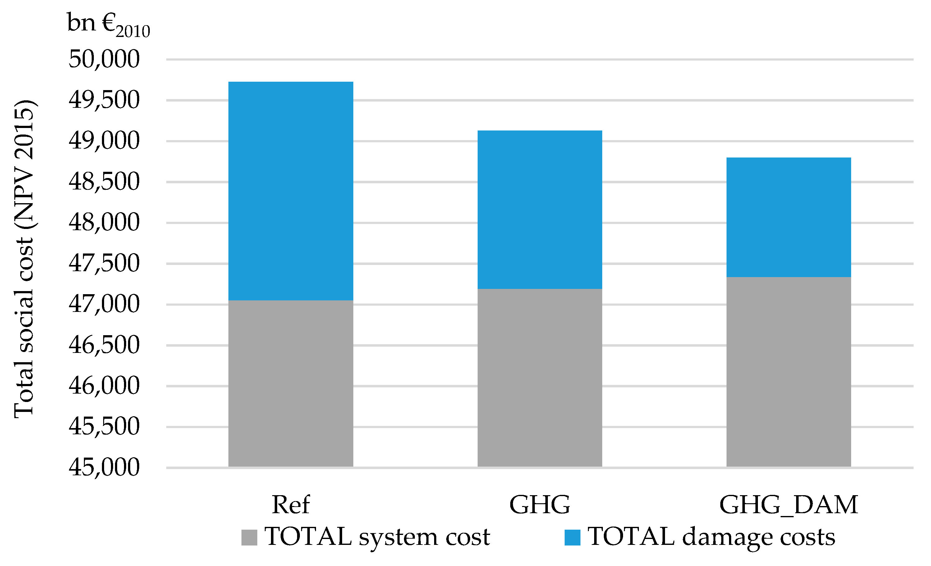
Including health damage cost in the optimization function brings early reductions not only on the health damage costs themselves but also on CO2 mitigation costs. Simultaneously considering decarbonization targets and air pollutants and their health damage costs, further increases co-benefits. Although the decarbonization target already decreases the level of air pollutants and their health damage costs, internalizing these costs in the energy system accelerates this reduction in the early periods and brings further reductions—also in CO2 emissions—in the residential sector and industry. The system can benefit from the immediate effects, whereas CO2 reduction targets rather determine the middle and long term actions. Having such a system also provides insights from the utilization of different energy carriers. Biomass can be given as an example. Although biomass is considered as CO2 free, having health damage cost in the optimization function can change their utilization in different sectors because of associated emissions of particulate matter. Integration of the health damage costs into the energy system analysis also reduces the total social cost by optimization the both total system cost and health damage costs from the pollutants. In the presented analysis, we only applied country-specific health damage cost factors, ignoring the differences in health impacts of different emission sources. Considering the ongoing discussion about air-quality issues, especially in cities and mainly caused by road transport, further disaggregating health damage costs for different emission sources may affect the effort sharing in GHG reductions between the different sectors. With regard to the different temporal effects of decarbonization targets and health damage costs of air pollution, a different implantation scheme could provide further insights on co-benefits and interactions. As an example, a slower and stepwise introduction of the health damage costs in the system (starting only in 2025, increasing gradually) could reflect a more realistic policy scenario and, in combination with the NEWAGE link, allows us to study the impact of a tax on air pollution in combination with an emission-trading system for GHG.
Energy transition changes the economic variables, such as GDP and sectoral production, and these variables have an impact on the energy-service demands in energy system. Energy service demands, especially in public transportation and industrial branches, are affected after the consideration of these economic variations in the energy system through the link with NEWAGE. This energy service demand change also brings reductions in final and primary energy consumption. As the energy service demands are mainly altered in industry and public transport, final energy consumption of these sectors experience the higher variations compared to other sectors. The impact from the economic variables in the system on the end user sectors such as commercial, agriculture, residential and private transport is limited, since these sectors also react less to the carbon cap and trade system in the macro-economic model. In the case of the commercial and agriculture sectors, they consume less fossil fuels than industrial sectors and are less vulnerable to CO2 prices. As for residential and private transport, they are matched to utility and net income in NEWAGE, respectively, according to Table A3 and these variables are not affected by the CO
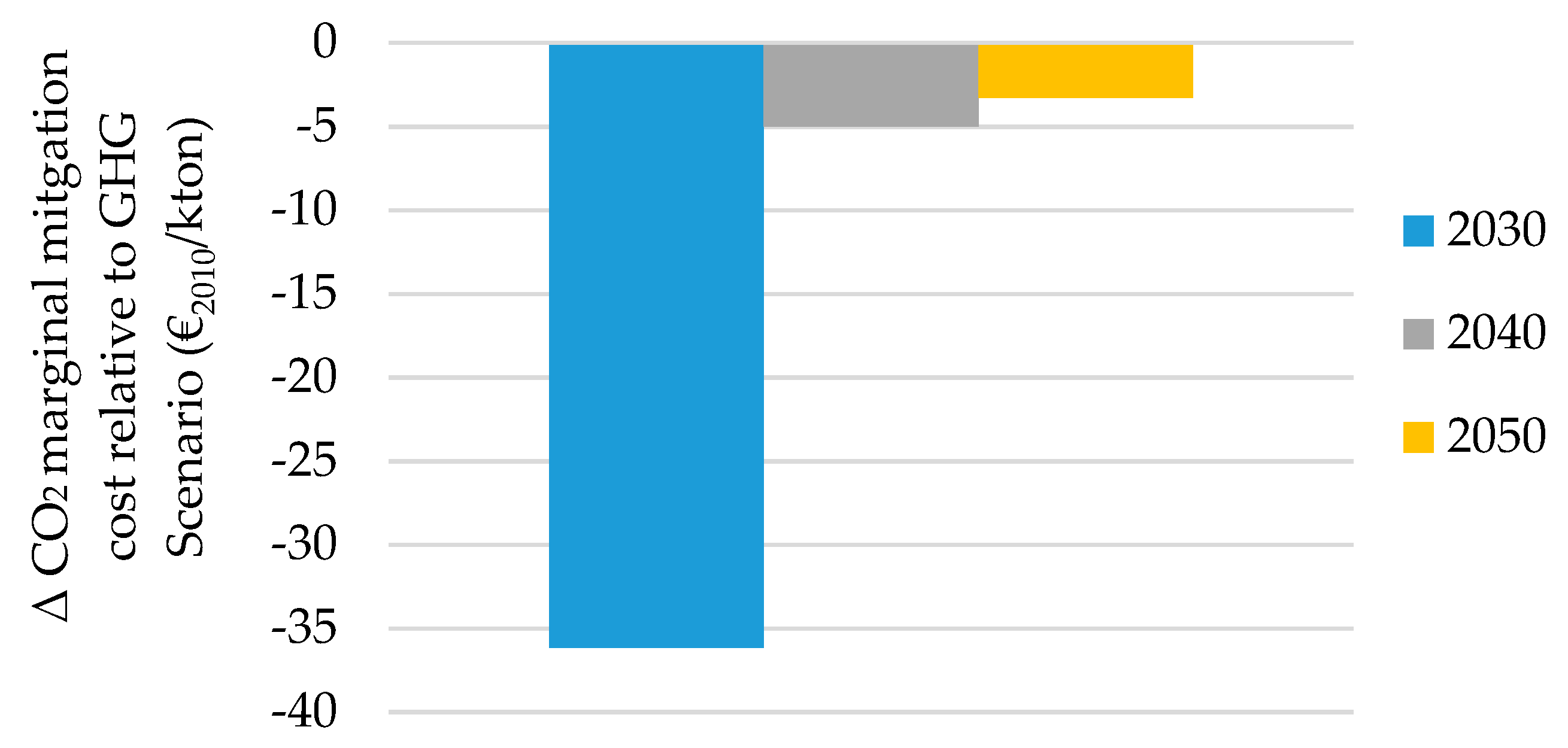
2 prices. For future coupling exercises, it is advised that the sectoral disaggregation of NEWAGE is further refined to better reflect the residential and private transport. With the reduction of renewables in the primary energy consumption, the role of renewables in the decarbonization also slightly diminishes and this is compensated for by the energy service demand change. Integration of economic variables enables the energy transition by also reducing the marginal CO2 mitigation cost.
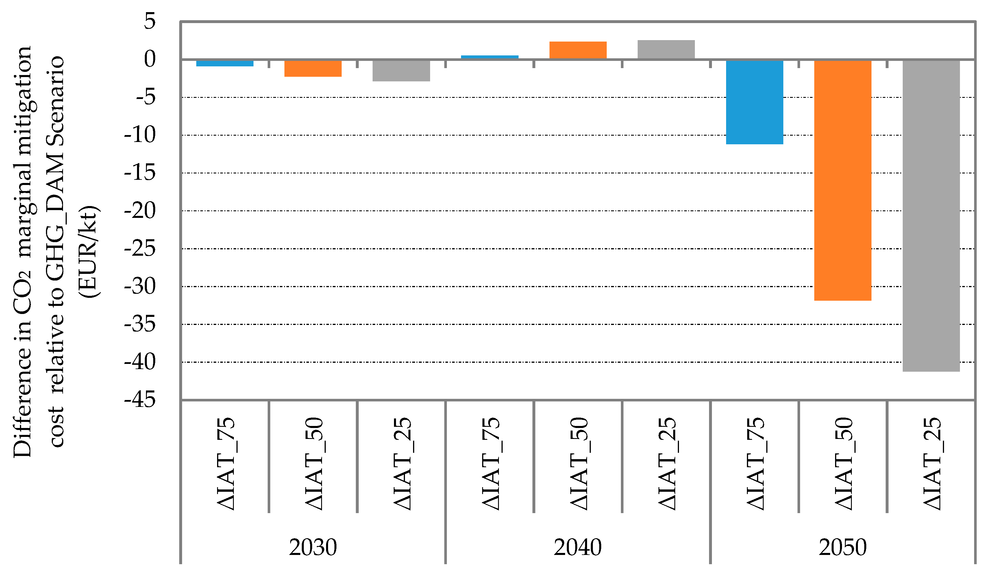
To analyze the role of the decoupling factor for the link between NEWAGE and TIMES PanEU, we carried out the iteration process with different decoupling factors. According to our findings, the decoupling factor does not only have an impact on the convergence values of the models but also on the iteration process. Having a decoupling factor of 50% or lower decreases the number of iterations needed to reach convergence but increases the impact on the results. The lower the decoupling factor, the tighter the link between the models. On the other hand, the iteration process took longer with 75% but exchanged data were not changed drastically compared to the reference case. Linking the two models can be a time-intensive task, especially in the early stages of harmonizing assumptions and matching sectors, but it also demands transparency from the modelers, which increases confidence in the entire process. After the required set-up, the linking process becomes also rather straightforward. Therefore, it can be applied in scenario analyses directly without increasing the complexity.
In our study, we did not develop any methodology to determine the decoupling factor but carried out sensitivity analyses to investigate the impacts. We suggest that a more elaborative method could be developed to determine such a factor as it has impacts on the results. Additionally, we believe that a link between the general equilibrium model and the impact assessment model can be considered for further research, which would allow for the analysis of health damage costs directly related to economic variations. Deeper coupling between NEWAGE and TIMES PanEU could be also possible by implementing more data from TIMES PanEU results as input to NEWAGE. The data exchange between the models can be also further elaborated in further research.
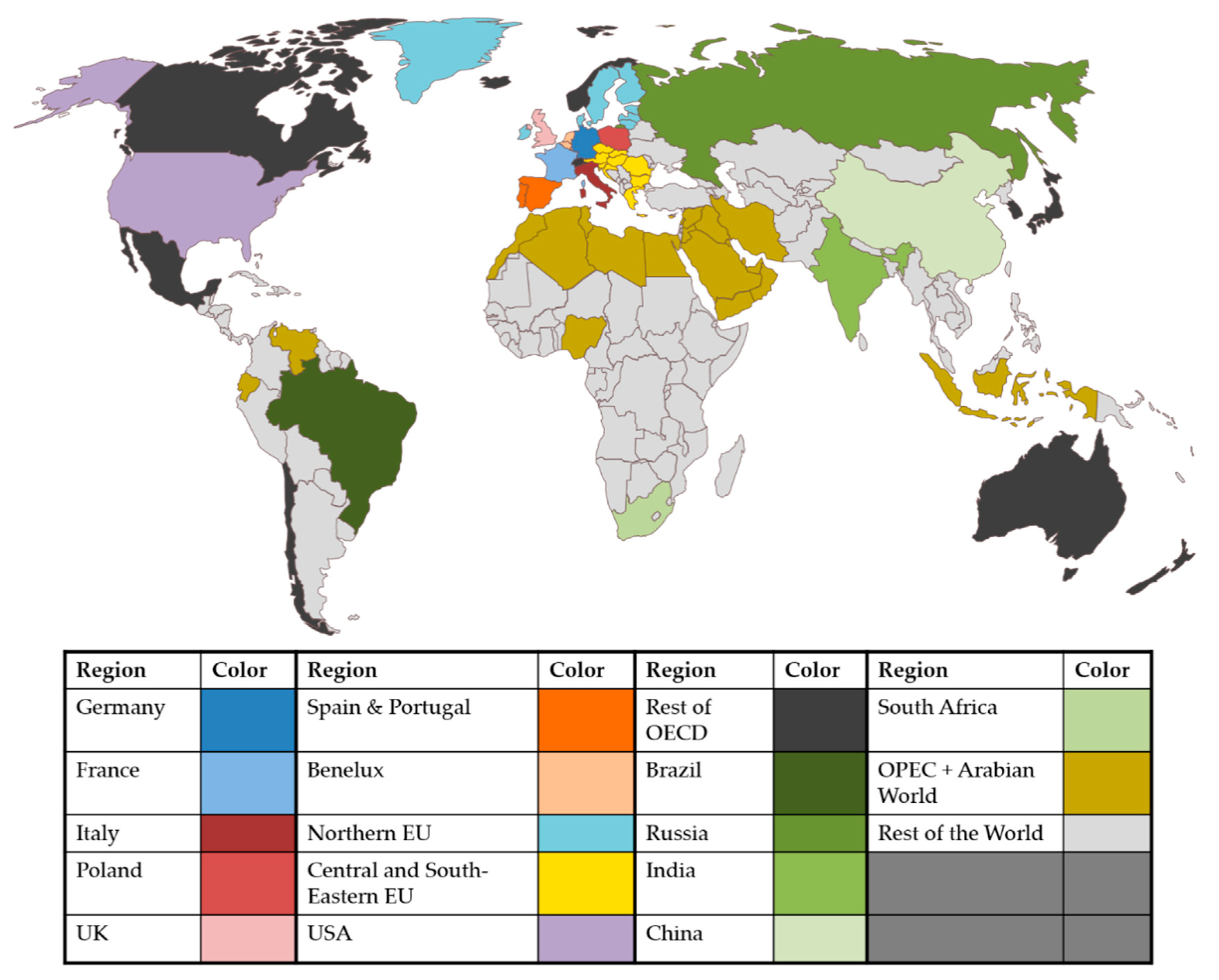
As NEWAGE is a global model and TIMES PanEU is a EU model, scenario assumptions are determined at the EU and global level. To determine the EU assumptions, the reduction target is set based on the discussed targets in [1], yet, at the time of this study, no global commitment to decarbonization existed. As trade between the regions is allowed in NEWAGE and decarbonization in one region might affect the dynamics in other regions, the assumptions for the rest of the world might affect the results in the EU. Therefore, a similar study with different global assumptions should be undertaken to assess the impact of different global assumptions. Additionally, we carried out this analysis at the EU level and did not focus on the individual member states. It might be possible to conclude different findings when the role of the demand change and externalities are considered in the energy system for the individual member states instead.
To investigate the role of different mitigation options together with the demand change, CO2 decomposition analysis was carried out for the whole system. Before this analysis, we also analyzed the sectoral CO2 reduction paths in each scenario. With the integration of health damage costs in the energy system, effort sharing between residential, commercial, agriculture and transport sectors slightly changed. Transport could reduce slightly more while the others slightly increase their emissions. The role of effort-sharing between the sectors is also observed after the integration of demand change. Due to higher reductions in industry; agriculture, commercial and agriculture could emit more. An increased share of renewables dominates but this share slightly reduces after the integration of service demand change in the decomposition analysis. In our study, the service-demand change is provided with the link of a general equilibrium model as an additional improvement to the existing literature. Integration of economic variables helps to reduce the structural change in the energy system through the energy transition. According to the remaining CO2 emissions, transport is identified as hardest to decarbonize between the non-ETS sectors. To also investigate the sector dynamics, decomposition analysis is also carried out specifically in the transport sector. Service demand change has a higher impact after the integration of macro-economic variables compared to the overall system in this sector and the main mitigation options appear to be biofuels and electricity. We also suggest as further research analyzing the role of the specific mitigation options in each sector by carrying out decomposition analysis. As the uncertainty also appears with the cost of the mitigation technologies and availability of the sources, further analysis should also address the impact of such uncertainties. Furthermore, different EU countries may prioritize different mitigation options to decarbonize their system based on their existing energy system. It is also seen in our analysis that some of the countries prefer to deploy more renewables, while others favor sticking with fossil fuels by applying options to reduce their carbon-content such as CCS. Therefore, as a further research, we suggest also investigating decomposition analysis at the Member States level to gain more insights for the further development of their energy system during the energy transition.
Based on our analysis, implementing the economic variations and health damage costs and considering these in scenario construction determines different CO2 reduction paths as it is seen in the decomposition analysis. Instead of the isolated energy system, it will also be important to take into account these elements outside the energy system during the energy transition. With this analysis, we showed a more complete picture of the energy transition together with these elements. Reducing GHG emissions does not only affect the system itself but the whole economy and society. A comprehensive analysis including economic variations and impacts on society in the form of reduced health costs allows us to account for co-benefits and interactions with economic mechanisms such as a carbon cap and trade system. This integrated view can provide valuable insights to determine efficient and effective decarbonization paths as well as increase awareness of interactions and side effects, which may help to increase acceptance of specific, necessary changes.

Author Contributions

Conceptualization, P.K., R.C.M., D.S. and U.F.; Methodology, P.K., R.C.M. and D.S.; Formal analysis, P.K., R.C.M. and D.S.; Investigation, P.K. and R.C.M.; writing—original draft preparation, P.K. and R.C.M.; Writing—review and editing, P.K., R.C.M., D.S., U.F. and M.B.; visualization, P.K. and R.C.M.; supervision, P.K., R.C.M., M.B. and U.F.; Project administration, U.F. All authors have read and agreed to the published version of the manuscript.

Funding

This research received no external funding.

Acknowledgments

The initial concept of this study was developed in the project “REEEM” funded by European Union’s Horizon 2020 research and innovation program under grant agreement No 691739.

Conflicts of Interest

The authors declare no conflict of interest.

Appendix A

Figure A1. Regional disaggregation in NEWAGE. Each region in the model has its own color in the map.
Energies 13 00707 g0a1
Table A1. List of production sectors in NEWAGE.
No.SectorGroup
1CoalEnergy production
2Natural gasEnergy production
3Crude oilEnergy production
4Oil refiningEnergy production
5ElectricityEnergy production
6Iron and SteelEnergy intensive industries
7Non-ferrous metalsEnergy intensive industries
8Non-metallic mineralsEnergy intensive industries
9Paper, pulp and printEnergy intensive industries
10ChemicalsEnergy intensive industries
11Food and TobaccoEnergy intensive industries
12Motor vehiclesOther manufacturing
13MachineryOther manufacturing
14Rest of industryOther manufacturing
15BuildingsRest of the economy
16TransportRest of the economy
17AgricultureRest of the economy
18ServicesRest of the economy
Figure A2. CES structure in NEWAGE for the production sectors.
Energies 13 00707 g0a2
Figure A3. CES structure in NEWAGE for electricity production.
Energies 13 00707 g0a3

Regional Push

The regional push scenario can be translated as the mutual work of several regions that, together, concentrate at least half of the global emissions and have the economic means to pursue emission targets that are consistent with the 2 °C target, according to the 2DS path presented in [39], or at least more ambitious than the current policies, as shown in the RTS path presented in [39].
Since the EU-28 has specific emission targets, Table A2 depicts only the emission targets of NEWAGE’s regions outside of the EU that pursue a higher emission cut than the current policies in the Regional Push World state.
Table A2. Emission targets for regions outside of the EU-28 pursuing emission cuts higher than the current policies for the regional push world state.
RegionCO2 Emission Targets in 2050
USAHalfway between 2 °C target and current policies
China2 °C target
JapanHalfway between 2 °C target and current policies
Republic of Korea2 °C target
CanadaHalfway between 2 °C target and current policies
MexicoHalfway between 2 °C target and current policies
AustraliaHalfway between 2 °C target and current policies
Norway80% reduction compared to 1990 levels
Switzerland80% reduction compared to 1990 levels
New Zealand2 °C target
Iceland2 °C target

Appendix B

Table A3. The sectoral match between TIMES PanEU and NEWAGE.
TIMES PanEUNEWAGE
AGRAgriculture
Commercial Cooling largeServices
Commercial CookingServices
Commercial Cooling smallServices
Commercial Heating largeServices
Commercial Heating smallServices
Commercial LightingServices
Commercial Other electricityServices
Commercial Other energyServices
Commercial Public lightingServices
Commercial RefrigerationServices
Commercial Water heat largeServices
Commercial Water heat smallServices
Aluminum Non-ferrous metal
AmmoniaChemistry
Other chemical Chemistry
ChlorineChemistry
Cement Non-metallic minerals
Copper Non-ferrous metal
Food and Tobacco Food and Tobacco
Glass Flat Non-metallic minerals
Glass Hollow Non-metallic minerals
Iron and SteelIron and Steel
Lime Non-metallic minerals
Other non-ferrous metalsNon-ferrous metal
Other non-metallic mineralsNon-metallic minerals
Other industriesRest of Industry
High-Quality paper Paper Pulp Print
Non energy-consumption chemicals Chemistry
Non energy-consumption others Non-metallic minerals
Other Sector Consumption Services
Other electricity GDP
Road Transport (Short- Long-Distance)Net Income
MotorcycleNet Income
Bus/Train (Public Transport) Transport
Truck (Freight)Transport
Rail Freight Transport
Aviation (Internal/External)Transport
Navigation (Internal/External)Navigation
Residential Space Heating Multi, Urban, RuralUtility
Residential Space Cooling Multi, Urban, RuralUtility
Residential Water HeatUtility
Residential CookingUtility
Residential Cloth Washing and DryingUtility
Residential LightingUtility
Table A4. Electricity technology match NEWAGE and TIMES PanEU.
NEWAGETIMES-PanEU Technologies
TechnologyLoadTechnology
NuclearBaseNuclear
HydroBaseRun of River
PeakDam Storage; Pump Storage
GeothermalBaseGeothermal
SolarMediumSolar
WindMediumWind
Hard CoalBaseCoal—Steam Turbine (CHP)
MediumCoal—Steam Turbine (not CHP)
LigniteBaseLignite—Steam turbine
Oil ProductsBaseOil—Combined Cycle
MediumOil—Gas Turbine
PeakOil—Internal Combustion; Steam Turbine
Natural GasBaseNatural Gas—Combined Cycle
MediumNatural Gas—Gas Turbine
PeakNatural Gas—Steam Turbine; Internal Combustion
BiomassBaseWaste non-renewable; Biomass solid/Waste ren.; Biogas/Biofuel
CCSBaseCCS from Lignite
MediumCCS from Hardcoal

Appendix C

Appendix C.1. Total System—CO2 Decomposition Analysis

Figure A4. CO2 Decomposition (Mt)—total system in the EU28.
Energies 13 00707 g0a4

Appendix C.2. Transport—CO2 Decomposition Analysis

Figure A5. CO2 decomposition (Mt)—transport in the EU-28.
Energies 13 00707 g0a5

References

  1. European Commission. In-Depth Analysis in Support of the Commission Communication com (2018) 773: A Clean Planet for All - A European Long-Term Strategic Vision for a Prosperous, Modern, Competitive and Climate Neutral Economy 2018. Available online: https://ec.europa.eu/knowledge4policy/publication/depth-analysis-support-com2018-773-clean-planet-all-european-strategic-long-term-vision_en (accessed on 20 October 2019).
  2. Warr, B.; Ayres, R.; Eisenmenger, N.; Krausmann, F.; Schandl, H. Energy use and economic development: A comparative analysis of useful work supply in Austria, Japan, the United Kingdom and the US during 100years of economic growth. Ecol. Econ. 2010, 69, 1904–1917. [Google Scholar] [CrossRef]
  3. Schmid, D.; Korkmaz, P.; Blesl, M.; Fahl, U.; Friedrich, R. Analyzing transformation pathways to a sustainable European energy system—Internalization of health damage costs caused by air pollution. Energy Strategy Rev. 2019, 26, 100417. [Google Scholar] [CrossRef]
  4. Nakicenovic, N.; Alcamo, J.; Grubler, A.; Riahi, K.; Roehrl, R.A.; Rogner, H.H.; Victor, N. Special Report on Emissions Scenarios: A special Report of Working Group III of the Intergovernmental Panel on Climate Change; Cambridge University Press: Cambridge, UK; New York, NY, USA, 2000; ISBN 978-0-521-80081-5. [Google Scholar]
  5. Messner, S.; Schrattenholzer, L. MESSAGE–MACRO: Linking an energy supply model with a macroeconomic module and solving it iteratively. Energy 2000, 25, 267–282. [Google Scholar] [CrossRef] [Green Version]
  6. Labriet, M.; Joshi, S.R.; Vielle, M.; Holden, P.B.; Edwards, N.R.; Kanudia, A.; Loulou, R.; Babonneau, F. Worldwide impacts of climate change on energy for heating and cooling. Mitig. Adapt. Strateg. Glob. Chang. 2015, 20, 1111–1136. [Google Scholar] [CrossRef] [Green Version]
  7. Kypreos, S.; Blesl, M.; Cosmi, C.; Kanudia, A.; Loulou, R.; Smekens, K.; Salvia, M.; Van Regemorter, D.; Cuomo, V. TIMES-EU: A Pan-European model integrating LCA and external costs. Int. J. Sustain. Dev. Plan. 2008, 3, 180–194. [Google Scholar] [CrossRef]
  8. Pietrapertosa, F.; Cosmi, C.; Di Leo, S.; Loperte, S.; Macchiato, M.; Salvia, M.; Cuomo, V. Assessment of externalities related to global and local air pollutants with the NEEDS-TIMES Italy model. Renew. Sustain. Energy Rev. 2010, 14, 404–412. [Google Scholar] [CrossRef]
  9. Kesicki, F. Marginal Abatement Cost Curves: Combining Energy System Modelling and Decomposition Analysis. Environ. Model. Assess. 2013, 18, 27–37. [Google Scholar] [CrossRef]
  10. Akbostancı, E.; Tunç, G.İ.; Türüt-Aşık, S. CO2 emissions of Turkish manufacturing industry: A decomposition analysis. Appl. Energy 2011, 88, 2273–2278. [Google Scholar] [CrossRef]
  11. Mousavi, B.; Lopez, N.S.A.; Biona, J.B.M.; Chiu, A.S.F.; Blesl, M. Driving forces of Iran’s CO2 emissions from energy consumption: An LMDI decomposition approach. Appl. Energy 2017, 206, 804–814. [Google Scholar] [CrossRef]
  12. Blesl, M.; Kober, T.; Kuder, R.; Bruchof, D. Implications of different climate protection regimes for the EU-27 and its member states through 2050. Clim. Policy 2012, 12, 301–319. [Google Scholar] [CrossRef]
  13. Simoes, S.; Nijs, W.; Ruiz, P.; Sgobbi, A.; Thiel, C. Comparing policy routes for low-carbon power technology deployment in EU – an energy system analysis. Energy Policy 2017, 101, 353–365. [Google Scholar] [CrossRef]
  14. Remme, U. Overview of TIMES: Parameters, Primal Variables & Equations. Available online: https://www.ier.uni-stuttgart.de/publikationen/pb_pdf/Remme_Overview_TIMES_2007.pdf (accessed on 11 February 2019).
  15. Gagiulo, M.; Vailancourt, K.; De Miglio, R. Documentation for the TIMES Model Part IV 2016. IEA Energy Technol. Syst. Anal. Programme 2016, 1–78. [Google Scholar]
  16. Loulou, R.; Remme, U.; Kanudia, A.; Lehtila, A.; Goldstein, G. Documentation for the TIMES Model Part I. IEA Energy Technol. Syst. Anal. Programme 2004, 1–78. [Google Scholar]
  17. Unger, T. Nordic Energy Perspectives (projekt). Coordinated Use of Energy System Models in Energy and Climate Policy Analysis: Lessons Learned from the Nordic Energy Perspectives Project; Profu: Mölndal, Sweden, 2010; ISBN 978-91-978585-9-5. [Google Scholar]
  18. International Energy Agency. World Energy Outlook 2016; OECD: Paris, France, 2016; ISBN 978-92-64-26494-6. [Google Scholar]
  19. Ruiz, P.; Sgobbi, A.; Nijs, W.N.; Thiel, C.; Dalla Longa, F.; Kober, T.; Elbersen, B.; Hengeveld, G.; European Commission; Joint Research Centre. The JRC-EU-TIMES Model: Bioenergy Potentials for EU and Neighbouring Countries; Publications Office: Luxembourg, 2015; ISBN 978-92-79-53879-7. [Google Scholar]
  20. Welsch, J. Modellierung von Energiespeichern und Power-to-X- im deutschen und europäischen Energiesystem; University of Stuttgart: Stuttgart, Germany, 2018. [Google Scholar] [CrossRef]
  21. Kuder, R. Energieeffizienz in der Industrie: Modellgestützte Analyse des effizienten Energieeinsatzes in der EU-27 mit Fokus auf den Industriesektor; University of Stuttgart: Stuttgart, Germany, 2014. [Google Scholar] [CrossRef]
  22. Directorate-General for Energy and Transport; Directorate-General for Climate Action; Directorate-General for Mobility and Transport. EU Reference Scenario 2016: Energy, Transport and GHG Emissions - Trends to 2050; Publications Office of the European Union: Luxembourg, 2016; ISBN 978-92-79-52374-8. [Google Scholar]
  23. Meyer, G.; European Commission; Directorate-General for Research and Innovation. Electrification of the Transport System Expert Group Report; European Commission: Brussels, Belgium, 2017; ISBN 978-92-79-71856-4. [Google Scholar]
  24. ExternE: Externalities of Energy; Methodology 2005 Update; Bickel, P.; European Commission (Eds.) EUR; Office for Official Publications of the European Communities: Luxembourg, 2005; ISBN 978-92-79-00423-0. [Google Scholar]
  25. Roos, J. Ermittlung und Bewertung von vermiedenen Gesundheitsschäden im Rahmen der Technikbewertung; Univesity of Stuttgart: Stuttgart, Germany, 2017; Available online: https://elib.uni-stuttgart.de/handle/11682/9194 (accessed on 15 September 2019).
  26. Friedrich, R.; Kuhn, A. D 5.3.1/2 Methods and results of the HEIMTSA/INTARESE Common Case Study; Stuttgart, Germany. Available online: http://www.integrated-assessment.eu/eu/sites/default/files/CCS_FINAL_REPORT_final.pdf (accessed on 10 October 2019).
  27. Simpson, D.; Benedictow, A.; Berge, H.; Bergström, R.; Emberson, L.D.; Fagerli, H.; Flechard, C.R.; Hayman, G.D.; Gauss, M.; Jonson, J.E.; et al. The EMEP MSC-W chemical transport model – technical description. Atmospheric Chem. Phys. 2012, 12, 7825–7865. [Google Scholar] [CrossRef] [Green Version]
  28. Wind, P.; Simpson, D.; Tarrasón, L. EMEP Status Report 1/2004; Source-Receptor Calculations; Norwegian Meteorological Institute: Oslo, Norway, 2004. [Google Scholar]
  29. Héroux, M.-E.; Anderson, H.R.; Atkinson, R.; Brunekreef, B.; Cohen, A.; Forastiere, F.; Hurley, F.; Katsouyanni, K.; Krewski, D.; Krzyzanowski, M.; et al. Quantifying the health impacts of ambient air pollutants: Recommendations of a WHO/Europe project. Int. J. Public Health 2015, 60, 619–627. [Google Scholar] [CrossRef] [PubMed] [Green Version]
  30. Holland, M. Implementation of the HRAPIE Recommendations for European Air Pollution CBA Work. 2014. Available online: https://ec.europa.eu/environment/air/pdf/CBA%20HRAPIE%20implement.pdf (accessed on 9 December 2019).
  31. Batista e Silva, F.; Gallego, J.; Lavalle, C. A high-resolution population grid map for Europe. J. Maps 2013, 9, 16–28. [Google Scholar] [CrossRef]
  32. Schmid, D.; Im, U. Focus Report on Health Impacts and External Costs due to Air Pollution; REEEM Deliverables. 2019. Available online: https://zenodo.org/record/3355829#.XfESy5NKi70 (accessed on 12 January 2019).
  33. Beestermöller, R. Die Energienachfrage privater Haushalte und ihre Bedeutung für den Klimaschutz: volkswirtschaftliche Analysen zur deutschen und europäischen Klimapolitik mit einem technologiefundierten Allgemeinen Gleichgewichtsmodell; University of Stuttgart: Stuttgart, Germany, 2017. [Google Scholar] [CrossRef]
  34. Cunha Montenegro, R.; Lekavičius, V.; Brajković, J.; Fahl, U.; Hufendiek, K. Long-Term Distributional Impacts of European Cap-and-Trade Climate Policies: A CGE Multi-Regional Analysis. Sustainability 2019, 11, 6868. [Google Scholar] [CrossRef] [Green Version]
  35. European Commission. Communication From The Commission To The European Parliament, The Council, The European Economic And Social Committee And The Committee Of The Regions A Clean Air Programme for Europe. 2013. Available online: https://eur-lex.europa.eu/legal-content/EN/TXT/?uri=CELEX%3A52013DC0918 (accessed on 12 January 2019).
  36. Loulou, R.; Lehtila, A. TIMES Damage functions; Energy Technology Systems Analysis Programme (ETSAP). 2015. Available online: http://iea-etsap.org/docs/TIMES-Damage.pdf (accessed on 10 November 2019).
  37. Labriet, M.; Drouet, L.; Vielle, M.; Haurie, A.; Kanudia, A.; Loulou, R. Coupled Bottom-Up and Top-Down Modelling to Investigate Cooperative Climate Policies. 2010. Available online: https://www.epfl.ch/labs/gemini-e3/wp-content/uploads/2018/08/Coupled-Bottom-Up-and-Top-Down-Modelling-to-Investigate-Cooperative-Climate-Policies (accessed on 12 September 2019).
  38. Moreau, V.; Vuille, F. Decoupling energy use and economic growth: Counter evidence from structural effects and embodied energy in trade. Appl. Energy 2018, 215, 54–62. [Google Scholar] [CrossRef]
  39. IEA (International Energy Agency). Energy Technology Perspectives 2017; OECD/IEA: Paris, France, 2017; ISBN 978-92-64-27597-3. [Google Scholar]
  40. Schmidt, O.; Hawkes, A.; Gambhir, A.; Staffell, I. The future cost of electrical energy storage based on experience rates. Nat. Energy 2017, 2, 17110. [Google Scholar] [CrossRef]
  41. ENTSO-E. TYNDP. 2018. Available online: https://tyndp.entsoe.eu/tyndp2018/ (accessed on 20 January 2019).
  42. United Nations Framework Convention on Climate Change (UNFCCC). The Paris Agreement. Available online: https://unfccc.int/process-and-meetings/the-paris-agreement/the-paris-agreement (accessed on 10 October 2019).
  43. Korkmaz, P.; Blesl, M.; Fahl, U.; Balyk, O.; Petrovic, S.; Simonsen, M.B.; Henke, H. REEEM-D6.1_Integrated Energy System Model; REEEM Project: Stockholm, Sweden, 2019. [Google Scholar] [CrossRef]
  44. Darmani, A.; Sanz, J.; Simonot, E.; Avgerinopoulos, G.; Gardumi, F. D2.1b. REEEM Innovation and technology Roadmap Renewable Energy Integration: Analysis of Wind, Solar PV and Ocean Energy. Available online: https://zenodo.org/record/3368433#.XfEd0ZNKi70 (accessed on 12 May 2019).
Figure 1. The Integrated Assessment Toolbox.
Energies 13 00707 g001
Figure 2. Integrated Assessment Toolbox—links between the models.
Energies 13 00707 g002
Figure 3. Difference in annual costs of air pollution relative to the reference scenario in the European Union (EU28, bn €2010).
Energies 13 00707 g003
Figure 4. Difference in marginal CO2 mitigation cost in greenhouse gas damage (GHG_DAM) scenario and greenhouse gas (GHG) scenario in the EU28 (€2010/kton).
Energies 13 00707 g004
Figure 5. Total social cost in the EU28 (bn €, 2010).
Energies 13 00707 g005
Figure 6. Values of selected economic variables in the EU28 for GHG_DAM compared to the reference scenario.
Energies 13 00707 g006
Figure 7. Difference (%) in the selected energy service demand developments in the EU28 compared to previous iteration for (a) IAT_50 and (b) IAT_75 in 2050.
Energies 13 00707 g007
Figure 8. Difference (%) in electricity generation in the EU28 compared to previous iteration for (a) IAT_50 and (b) IAT_75 in 2050.
Energies 13 00707 g008
Figure 9. Difference in annual final energy consumption by sector relative to GHG_DAM scenario in the EU28 (PJ).
Energies 13 00707 g009
Figure 10. Difference in primary energy production relative to GHG_DAM scenario in the EU28 (PJ).
Energies 13 00707 g010
Figure 11. Difference in CO2 marginal mitigation cost relative to GHG_DAM Scenario in the EU28 (€/kt).
Energies 13 00707 g011
Figure 12. Difference of selected economic variables in the EU28 compared to GHG_DAM in 2050.
Energies 13 00707 g012
Figure 13. Sectoral CO2 emission reductions relative to 2015 emissions in the EU28 (black squares refer to the relative CO2 reduction targets according to 2015 level to be achieved in 2030 and 2050).
Energies 13 00707 g013
Figure 14. Shares of different mitigation options in CO2 decomposition analysis compared to reference scenario in different scenarios in the EU28 in 2050.
Energies 13 00707 g014
Figure 15. Shares of different mitigation options in CO2 decomposition analysis in different scenarios in the EU28 in 2050—transport sector.
Energies 13 00707 g015
Table 1. Milestone targets of the analyzed reduction scenario.
YearGHG Reduction Target Milestones Rel. to 1990 LevelsGHG Reduction Target Milestones Rel. to 2015 Levels
203050%35%
204070%55%
205085%81%
Table 2. Modelled scenarios and their abbreviations.
AbbreviationDescriptionApplied Models
ReferenceBusiness as usual (EU reference scenario)TIMES PanEU; NEWAGE
GHG85% GHG reductionTIMES PanEU
GHG_DAM85% GHG reduction in the EU28 and health damage costs are internalized as part of the optimization function (ex-ante)TIMES PanEU + EcoSense; NEWAGE
IAT_2585% GHG reduction in the EU28, health damage costs are internalized as part of the optimization function (ex-ante), 25% decoupling factorIAT 1
IAT_5085% GHG reduction in the EU28, health damage costs are internalized as part of the optimization function (ex-ante), 50% decoupling factorIAT 1
IAT_7585% GHG reduction in the EU28, health damage costs are internalized as part of the optimization function (ex-ante), 75% decoupling factorIAT 1
1 TIMES PanEU + EcoSense + NEWAGE.
Table 3. Deviation of gross domestic product (GDP) between iterations for three decoupling factors.
Scenario123456
IAT_25- −0.3501% −0.0164% 0.0011% −0.0020% −0.0005%
IAT_50- −0.2816% 0.0051% 0.0028% −0.0042% 0.0014%
IAT_75- −0.2181% 0.1326% −0.1189% −0.0063% 0.0021%
Table 4. Difference in selected energy service demands and GDP relative to GHG_DAM scenario in 2050 in the EU28.
ScenariosTIMES PanEUNEWAGE
FreightNECIISGDP
Δ IAT_75−4.72%−3.10%−4.74%−0.21%
Δ IAT_50−9.43%−6.21%−9.51%−0.28%
Δ IAT_25−14.08%−9.30%−1.,24%−0.37%

