Efficiency Optimization and Control Strategy of Regenerative Braking System with Dual Motor


1
State Key Laboratory of Mechanical Transmission, Chongqing University, Chongqing 400044, China
2
School of Automotive Engineering, Chongqing University, Chongqing 400044, China
*
Author to whom correspondence should be addressed.
Energies 2020, 13(3), 711; https://doi.org/10.3390/en13030711
Submission received: 10 January 2020
/
Revised: 31 January 2020
/
Accepted: 5 February 2020
/
Published: 6 February 2020
(This article belongs to the Special Issue Energy Storage Systems for Electric Vehicles)
Abstract
:The regenerative braking system of electric vehicles can not only achieve the task of braking but also recover the braking energy. However, due to the lack of in-depth analysis of the energy loss mechanism in electric braking, the energy cannot be fully recovered. In this study, the energy recovery problem of regenerative braking using the independent front axle and rear axle motor drive system is investigated. The accurate motor model is established, and various losses are analyzed. Based on the principle of minimum losses, the motor control strategy is designed. Furthermore, the power flow characteristics in electric braking are analyzed, and the optimal continuously variable transmission (CVT) speed ratio under different working conditions is obtained through optimization. To understand the potential of dual-motor energy recovery, a regenerative braking control strategy is proposed by optimizing the dynamic distribution coefficient of the dual-electric mechanism and considering the restrictions of regulations and the I curve. The simulation results under typical operating conditions and the New York City Cycle (NYCC) proposed conditions indicate that the improved strategy has higher joint efficiency. The energy recovery rate of the proposed strategy is increased by 1.18% in comparison with the typical braking strategy.
1. Introduction
Given the limitations of oil resources and the importance of environmental protection, governments around the world have enacted stringent regulations on fuel consumption and emissions. Electric vehicles, as environmentally friendly vehicles, have attracted a considerable amount of attention from researchers and corporations, and regenerative braking technology as one of the key technologies of energy conservation and emission reduction has been widely studied and applied [1,2,3]. The regenerative braking system can use the motor to convert the braking kinetic energy into electric energy and store it in the battery. This electric energy can be released during the driving process, which can not only improve the energy utilization rate and extend the driving range but also reduce the driver’s range anxiety. Therefore, maximization of the braking energy recovery under safe braking conditions has been the focus and challenge of energy management of electric vehicles.
Zhang et al. proposed an improved regenerative braking control strategy for rear-drive electric vehicles. In the deceleration braking test, the improved regenerative braking efficiency could reach 47% [4]. Cheng et al. verified a new series control strategy, and the experimental results confirmed that the steady and dynamic contribution of the strategy to the improvement of energy efficiency reached 58.56% and 69.74%, respectively [5]. Itani et al. compared flywheels with supercapacitors as the second energy source of front axle driven electric vehicles, and the results demonstrated that ultra-capacitors performed better in weight, specific energy and specific power. It was more convenient to reuse the braking energy and provided a solution to reduce the damage of the large current to batteries during regenerative braking [6]. For the control of specific components, Yuan et al. proposed a new scheme of the line control dynamic system considering the functional requirements of regenerative braking in the structural development stage and adopted the current amplitude modulation control to improve the accuracy of hydraulic regulation and eliminate vibration noise. The maximum regeneration efficiency of the bench test was 46.32% of the total recoverable energy [7]. Chen proposed a feedback hierarchical controller that tracked the desired speed and distributed the braking torque to four wheels to improve the energy recovery [8]. In terms of overall optimization, Deng et al. analyzed the relationship between the battery, motor, CVT and comprehensive efficiency, and proposed a regenerative braking control strategy for the CVT hybrid electric vehicle. In comparison with the typical strategy, the average power generation efficiency of the motor increased by 2.91% [9]. Shu et al. developed a maximum energy recovery energy management strategy and used the sequential quadratic programming (SQP) algorithm to optimize the CVT ratio control strategy, which achieved a good control effect [10]. To expand the scope of braking energy recovery, Bera et al. used the motor and hydraulic system to jointly adjust the braking process of an anti-lock braking system (ABS) and obtained a good effect [11]. The above literatures have all conducted relevant studies on the improvement of energy recovery in the regenerative braking process, which has improved the regenerative braking performance of vehicles. However, there are a greater number of studies on a single model than on a joint model and more studies on regenerative braking of a single motor than on regenerative braking of vehicles with a dual-motor drive system.
As a key device of the regenerative braking system, the efficiency of the motor directly affects energy recovery. Hence, improving the efficiency of the motor is conducive to the increase of energy recovery. Many scholars have conducted relevant studies on improving motor efficiency. Tripathi et al. conducted a detailed study on the model-based loss minimization algorithm (MLMA), and the results confirmed that this method could not only effectively improve motor efficiency but also exhibit good dynamic performance [12]. Uddin et al. used a model-based loss minimization algorithm (LMA) to compare the efficiency of permanent magnet synchronous motors based on direct torque flux linkage control (DTFC) and vector control (VC). The simulation results showed that the former had higher efficiency [13]. Inoue et al. studied the control performance of the permanent magnet synchronous motor (PMSM) drive system based on current control and direct torque control. Their results showed that the latter, combined with the control law of the M-T framework, had the advantages of control stability [14]. Wang et al. introduced the integral balance of the sine value of the torque angle such that the speed and the electromagnetic torque could be controlled to converge at the same time by adjusting the speed only once and to obtain the optimal dynamic response of the speed [15]. Vido and Le Ballois [16] and Lee et al. [17] also conducted relevant studies and improved the efficiency of the motor to a certain extent. The above literatures have conducted research on the efficiency of the motor and obtained various results. However, in the process of regenerative braking, it is necessary to analyze the influencing factors of motor loss to maximize system efficiency.
To minimize the power loss in the process of electric braking, this study analyses the automobile with an independent motor drive system of the front and rear axles. First, the accurate motor model is established, and various losses are analyzed. Based on the principle of minimum loss, the motor control strategy is designed. The characteristics of power flow in the electric braking process are analyzed, and the combined efficiency model of the front and rear axles is established. The optimal transmission ratio of CVT under different working conditions is obtained through optimization, and the input and output characteristics of the front and rear axles are analyzed. Finally, by optimizing the brake force distribution coefficient of the front and rear motors and considering the ECE regulations and I curve as the limit, a new control strategy of dual motor regenerative braking is proposed to maximize the energy recovery.
2. Hybrid Electric Vehicle System Structure and Parameters
In comparison with pure electric vehicles and fuel cell vehicles, hybrid electric vehicles are widely used in production and by consumers without the disadvantages of short driving range, long charging time, high fuel cell price and difficult hydrogen re-filling [18]. The structural schematic diagram of the hybrid vehicle system studied here is shown in Figure 1, and it should be noted that the schematic diagram is not the layout of the real vehicle.
This configuration can be driven by the engine alone or by the motor. During high power demand, the motor and the engine can work simultaneously to meet the needs of the vehicle. The front axle and rear axle of this configuration have motors, which can make the vehicle exhibit better dynamic performance in pure electric mode and can recover more energy when braking. The vehicle controller is responsible for collecting the speed, brake pedal, brake master cylinder pressure and other signals and corresponding responses. When the brake pedal signal is detected, the driving state of the car is quickly determined, and the control signal is sent to the lower controller through the controller area network (CAN) bus. The lower controller makes correlation identification according to the control signal and sends signals to the hydraulic control unit and motor control unit according to the established algorithm to complete the driver’s instructions. The vehicle parameters and component parameters are shown in Table 1.
3. Motor Loss Model and Control Strategy
3.1. Motor Loss Model
Permanent magnet synchronous motors with the high-power density and high-efficiency advantages of small volume and light quality have been widely used in new energy vehicles [19]. To obtain a more accurate model, it must be considered that the iron loss in the model is important. Hence, the equivalent iron loss resistance is introduced parallel to the magnetizing branch in the circuit [20], as depicted in Figure 2. Certain idealized conditions are assumed; for example, saturation is ignored, and the electromotive force is sinusoidal [18]. Motor losses mainly include mechanical losses, copper losses, iron losses and stray losses. Since stray losses are difficult to measure and control and account for a small percentage of the total loss [21], they are not considered in this study.
In steady-state, the voltage balance equation of the d-q axis is as follows:
Here, is the stator winding resistance, and are the d-q axis components of the stator voltage, and are the d-axis and q-axis current components, respectively, is the angular velocity of the stator, and and are the d-q axis components of the stator flux, respectively. The permanent magnet flux has the following relationship:
The electromagnetic torque can be calculated using Equation (5).
where is the number of pole pairs, and are the d-q axis magnetization current components, respectively, and and are the d-q axis inductance components, respectively. For surface-mounted permanent magnet synchronous motors, = .
Then, copper loss and iron loss can be calculated by the Equations (6) and (7), respectively.
When the motor is working, the load and power factor are the key factors influencing the size of the copper loss. Therefore, when the current speed and torque are given, the current optimal (minimum loss) can be obtained:
Mechanical loss has an approximately linear relationship with motor speed [22]. By setting the value of K as constant, the mechanical loss model of permanent magnet synchronous motor can be obtained:
3.2. Motor Control Strategy
The motor control method has an important influence on motor performance. Hence, it is necessary to improve it to get higher motor efficiency. In comparison with most conventional proportional-integral-derivative (PID) control method, to obtain better performance and reduce energy losses here, the motor speed loop adopts the sliding mode control and the current loop uses the minimum loss control method (LMA). The total efficiency of the former motor for is set as
It can be observed that the total efficiency is a quadratic function of the stator q-axis excitation current. By using the mathematical method, it is observed that there is always a value of , which can minimize the total loss under different torque and electric angular speed. When the motor loss is set to be the lowest, it is as follows:
The constraints are
The voltage state equation of the d-q axis can be obtained by calculating the time derivative of each side of the loss constraint as follows:
The elements , , , , and are, respectively:
If all the above influential elements depend on the motor parameters and state, assuming that the X and Y elements meet the braking requirements, the output equation of the controller can be expressed as follows:
To obtain the stable torque closed-loop output, the PI (Proportional-Integral) algorithm is used as follows:
where and can be brought into the above equation to get
The optimal PI parameters can be obtained after multiple debugging. The overall control model of the motor is shown in Figure 3.
The analysis shows that when the motor runs without load, the copper loss accounts for a small proportion, and the iron loss increases linearly with the increase of the speed. When the motor is loaded, the copper loss of the motor increases in square shape relative to the load torque, while the iron loss increases slowly. The efficiency of the former PMSM can be simulated in Simulink, as depicted in Figure 4.
4. Optimization of the Electric Braking Power Flow Efficiency and the Braking Force Distribution
4.1. Optimization of the Electric Braking Power Flow Efficiency
4.1.1. Power Flow Analysis of Electric Braking
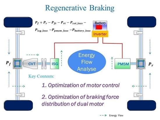
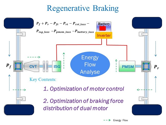
To improve the recovery of braking energy, it is necessary to analyze the loss of power flow in the process of electric braking. Here, the electric braking system is mainly composed of a front and rear motor, battery pack, CVT transmission, clutch and other vehicle parameters. The parameters of each component are shown in Table 1. Furthermore, as both front and rear motors can participate in the process, it means that more energy can be recovered, and the driving range can be effectively increased. The power flow of the vehicle’s electric braking loss is shown in Figure 5.
The overall efficiency of the vehicle’s electric brake energy recovery can be calculated using Equation (24):
Among them, is the total efficiency of the electric brake of the whole vehicle, and are the front and rear axle braking input powers, respectively; and are the front and rear axle transmission power losses, respectively; and are the power loss of the front and rear motors, respectively; is the CVT transmission loss; is the battery charging power loss.
As the power loss of the driving system is primarily related to the speed, whereas the loss of the motor and the inverter is a function of the electric angular speed and torque and the CVT loss is related to the input torque and the speed ratio, the equation can be rewritten as Equation (25).
where is the braking torque of the vehicle; is the distribution coefficient of forward and backward torque; and are the front and rear motor angular velocity, respectively; is the CVT transmission speed ratio; is the speed; is the CVT-ISG combined loss; is the loss of the rear motor; is the loss of the transmission system; and is the loss of the battery.
4.1.2. Establishment of the Joint Efficiency Model and Optimization of the CVT Speed Ratio
The combined front axle model is mainly composed of CVT and front motor and hence, its loss is calculated as Equation (26):
is the total power loss of the front axle. is the input torque of the front motor. and are CVT input and output speed, respectively. The torque loss of the CVT mainly includes the slip loss of the steel belt, the loss caused by the deformation of the belt wheel and the slip loss of the metal sheet [23]. When the speed is fixed at 2000 rpm, its efficiency changes, as shown in Figure 6. It can be observed that the efficiency of CVT is mainly related to the speed ratio. When the speed ratio is approximately 1, the efficiency reaches a maximum, but when it is less than 1, there is a significant decline in the efficiency.
Through the established CVT-ISG joint efficiency model, the CVT speed ratio with the highest joint efficiency can be determined. When the number ratio is 1.5, the joint efficiency changes are shown in Figure 7.
It can be found that the efficiency of the combined model in the region with high speed and low torque is lower than that of the single motor model. Since the CVT has lower efficiency in the region with low torque, it results in lower overall efficiency. Further, under different torques and rotating speeds, the combined efficiency changes with the CVT speed ratio. By seeking the CVT speed ratio that makes the combined efficiency reach maximum, the system efficiency can be maximized. The results are shown in Figure 8.
Therefore, by calculating the braking power of the motor through the pedal’s opening degree, the optimal CVT speed ratio under this braking torque can be obtained under the combined efficiency model. However, it should be noted that when the vehicle starts, the motor speed should be set greater than 500 rpm, and the speed ratio should be adjusted to the maximum to protect the motor from irreversible damage. When the vehicle is in an emergency braking state (z > 0.7), the CVT speed ratio should be adjusted to the minimum to ensure the safety and stability of the vehicle.
The rear axle joint model is mainly composed of a motor, which is relatively simple and similar to the front axle motor model. Therefore, it is not to be introduced separately.
4.1.3. Input and Output Characteristics of the Front and Rear Axis Joint Models
According to the joint model established above, the input and output characteristics of the front and rear axles are analyzed to provide a basis for formulating the braking force distribution strategy.
The braking strength allocated by the front axle during simulation is set to 0.3, and the energy recovery and energy consumption rate of the front axle braking system at different initial velocities are depicted in Figure 9.
It can be found that the higher the initial braking speed, the higher the energy recovery rate. This is because when the vehicle is at a higher speed, the motor is in an efficient working area, and the energy recovered is more than when it is at a lower speed. With the increase of the initial braking speed, the energy loss rate of the motor, CVT and battery decreases slowly, and the biggest loss is the motor loss. This indicates that the loss of the front axle is relatively small at higher speeds.
Under the same conditions, the characteristics of the rear axle joint model are depicted in Figure 10.
In comparison with the combined loss model of the front shaft, the recovery rate of the rear shaft is relatively higher, because there is no CVT to affect the efficiency of the motor, so the recovery rate is higher. Further, the loss rate of the rear shaft is lower than that of the front shaft, but the larger torque will cause the larger charging current of the battery, larger battery loss and lower charging efficiency.
4.2. The Braking Force Distribution Strategy with the Maximum Joint Efficiency
4.2.1. Front and Rear Motors Braking Force Distribution
Since the front and rear motors are different, it implies that the optimal operating range of the motor is different during the braking process. It is necessary to adjust the braking force of the front and rear motors to achieve a higher recovery rate. The utilization efficiency of regenerative braking of front and rear shafts is defined as follows:
where and are the braking power of the front and rear shafts, respectively. and are the combined braking efficiency of front and rear axles, respectively. A biaxial regenerative braking model was established.
where q is the braking force distribution coefficient of the rear axle; and are, respectively, the maximum braking power that the front and rear axles can provide. is the total regenerative braking power. The distribution coefficient of the optimal posterior axis is calculated as shown in Figure 11.
It can be observed that the surrounding dark blue part is the separate working area of the front motor during regenerative braking, the middle bright yellow part is the separate working area of the rear motor during regenerative braking and the remaining part is the joint working area of the front and rear axle joint model.
4.2.2. Vehicle Braking Force Distribution Strategy
Based on the above analysis, the mode switching point of regenerative braking of the front and rear axles can be obtained by fitting the boundary of the separate working area of the rear axles. Thus, the relationship between braking torque and speed is
As illustrated in Figure 12, when the regenerative braking torque of the vehicle is located in the envelope region of the curve and the coordinate axis, i.e., when , the rear axis is used for braking alone. When the braking torque is outside the curve, that is, , the braking force is allocated according to the p-value, and the peak power peak torque of the front and rear motors should be limited by the threshold value to prevent overload of the front and rear motors. Considering the braking stability and regulatory restrictions, the braking force distribution strategy is as follows:
(1) When z < 0.2, the braking force is distributed by the distribution coefficient of the rear shaft.
① Braking torque
is the rear axle braking force; is the braking force of the front axle; is the hydraulic braking force of the rear shaft; is the hydraulic braking force of the front shaft; is the vehicle radius; is the speed of the vehicle. At this point, the braking force will be provided by the rear motor alone. The front motor and the hydraulic braking system of the front and rear shafts do not participate in the braking.
② Braking torque
The braking force is distributed through the distribution coefficient q of the rear shaft. At this point, the front motor starts to participate in the regenerative braking, while the hydraulic braking system still does not participate in the braking.
When the braking strength is between 0.15 and 0.8, the Economic Commission of Europe (ECE) regulations stipulate that the curve of the rear axle using the adhesion coefficient should not be above the front axle. Hence, if the set distribution is reasonable, it should be considered here. According to the braking force distribution strategy in this study,
The relationship between the braking value and ECE braking regulations can be obtained [22], and the relation curve between the braking force distribution coefficient and the braking intensity z can be illustrated as shown in Figure 13. When the speed is 30 km/h and 100 km/h, it can be seen that the curve changes within the range permitted by regulations.
The upper limit curve A is to ensure that the adhesion coefficient of the front axis meets the requirements. Curve B is to limit the locking order of the front and rear wheels of the car. When the value appears above curve B, the front wheels can always be locked to the rear wheels in braking. However, when the value is lower than the curve C, the adhesion coefficient of the rear axis will be insufficient and hence, the contact value should be kept above the curve C at all times.
(2)
At this point, the braking force will be distributed according to the I curve. If the braking torque provided by the front and rear motors is insufficient to meet the braking task, the remaining braking power required will be supplemented by the hydraulic braking system.
where represents the braking force distribution coefficient under the I curve.
(3) z > 0.5
When the braking strength is greater than 0.5, the braking stability is most important. Therefore, reducing the braking force of the motor at a constant speed gradually withdraws the motor from the braking work. Simultaneously, the missing braking force is supplemented by the hydraulic pressing force to ensure that when z = 0.7, the motor completely exits the braking, without affecting the hydraulic pressure to provide the full braking force in case of emergency braking. The specific allocation strategy is shown in Figure 14.
5. Vehicle Performance Simulation and Analysis
Based on the joint loss model, the simulation model of the whole system was established in Simulink/MATLAB, as shown in Figure 15. The simulation analysis was conducted under typical working conditions and cyclic working conditions, respectively, to verify the effectiveness of the strategy.
5.1. Simulation of Typical Braking Conditions
The initial condition of the vehicle speed is 100 km/h and the SOC (State of charge) value of the power battery is 0.7. In addition, the influence of other resistances other than braking force, such as wind resistance, is not considered temporarily in the braking process. According to the analysis of power flow on the above analysis, the loss of each component in the braking process is made into an energy consumption diagram as shown in Figure 16.
5.1.1. Braking Strength z = 0.2
When the braking strength is 0.2, the change in SOC and the overall efficiency during the entire process from the beginning of braking to the end are depicted in Figure 17a and the loss of key components is depicted in Figure 17b.
It can be found that at the initial time, the joint efficiency decreases slowly, the efficiency is higher, and the energy can be fully recovered. According to the data in the figure, at this time, the loss of braking energy mainly comes from the motor. Since the front motor has a short working time, the focus is on the rear motor, which is the same as the CVT loss. It can be seen that 298.745 kJ energy has been recovered from the driver stepping on the brake pedal to the vehicle parking, 395.71 kJ energy has been lost and the recovery rate has reached 43.02%.
5.1.2. Braking Strength z = 0.4
When the braking strength is 0.4, the change in SOC and the overall efficiency during the entire process from the beginning of braking to the end are depicted in Figure 18a and the loss of key components is depicted in Figure 18b.
When the braking starts, the regenerative braking efficiency of the dual motors has a short period of platform area, and the efficiency is relatively high. As the speed decreases, the electric braking efficiency decreases, while the mechanical braking proportion increases. According to the data in the figure, due to the addition of hydraulic braking, the energy loss of most regenerative braking is hydraulic braking loss accounting for 69.06%. Both the front and rear motors are in the peak operating state. The loss of the front motor is higher than that of the rear motor due to the CVT, and the loss of the front and rear motors is smaller than that of the rear motor when the braking strength is 0.2 because the motor has a shorter working state.
5.1.3. Braking Strength z = 0.6
When the braking strength is 0.6, the change in SOC and the overall efficiency during the entire process from the beginning of braking to the end are depicted in Figure 19a and the loss of key components is depicted in Figure 19b.
It can be observed that at this point, due to the gradual withdrawal of the motor braking, the increase in SOC is not large. According to the data in the figure, the hydraulic braking loss accounts for a larger proportion, accounting for 85.64%. Furthermore, due to the short braking time, the overall loss of the front and rear motors decreases in comparison with the braking strength, and the CVT loss also decreases.
From the simulation of typical working conditions, it can be observed that despite the braking strength of 0.2, 0.4 or 0.6, the SOC increases to different degrees during the braking process, and the lower the braking strength and the longer the braking time under the same speed, the more energy will be recovered.
5.2. Cycle Simulation
To verify the distribution strategy in this study, NYCC was selected for cycle simulation, and the ideal braking force distribution method of motor first braking was compared. The braking torque, power, total system efficiency and SOC of the front and rear motors are analyzed. NYCC has the characteristics of low speed, high acceleration and frequent braking, and its braking environment and braking strength can be obtained as shown in Figure 20 [24].
The braking torque changes of the front and rear motors are depicted in Figure 21. To recover energy more efficiently, the rear motors often work in the state of peak torque, whereas the front motors often work in the state below the rated torque, so as to not be involved in braking as frequently as the rear motor.
The braking power changes of the front and rear motors are shown in Figure 22. It can be seen that the maximum power of the front motor is approximately 6.7 kW and that of the rear motor is approximately 14.8 kW. The braking frequency of the rear motor is relatively large. In comparison with the ideal braking strategy, the front motor did not participate in the braking in the early stage and the rear motor braking power increased.
The efficiency and SOC changes are depicted in Figure 23. The overall efficiency of the rear motor can reach approximately 0.8 when it works alone. As the selection of the CVT speed ratio can adjust the efficiency of the front motor, the overall efficiency of the front and rear motors is higher when they work together to effectively recover energy. After the complete working condition, the SOC rises by approximately 0.003.
From the changes in efficiency and SOC, it can be observed that under the condition of low braking strength, the braking force distribution method discussed here has a high recovery efficiency and can recover maximum energy. Additionally, the motor loss minimization algorithm was adopted to maximize the use of the front and rear motors, system efficiency and SOC were improved, and the energy recovery of NYCC increased by 1.18% in comparison with the typical braking strategy.
6. Conclusions
(1) In this study, the front axle and rear axle independent motor drive system vehicle was considered as the research objective, the accurate motor model was established, various losses were analyzed and a new motor control method was proposed based on the principle of minimum loss.
(2) The characteristics of power flow in the process of electric braking were analyzed in detail, the combined efficiency model of the front axle (CVT–ISG) and rear axle (PMSM) was established, the braking force distribution of the front and rear motors was optimized based on the input and output characteristics of the front and rear axles. It was found that the optimal braking force distribution coefficient of the front and rear axles will change with the change of the working conditions. According to this change rule, a dual-motor regenerative braking force distribution strategy based on the optimal braking energy recovery was designed.
(3) In the MATLAB/Simulink simulation platform, the double motor regenerative braking system model was developed, and the simulation analyze was carried out under three typical braking conditions and NYCC conditions, respectively. It was observed that when the braking strength was 0.2, the braking energy recovery rate could reach 43.02%, and the energy recovery rate of the improved strategy was 1.18% higher than that of the typical braking strategy under NYCC conditions, which verify the effectiveness of the strategy proposed in this study.
Author Contributions
Conceived the research ideas and put forward the research methods, Y.Y.; Build the model and simulated it, Q.H. and Y.C.; Analyzed the simulation data, C.F. All authors have read and agreed to the published version of the manuscript.
Funding
The research was supported by (1) the National Key R&D Program of China (grant No. 2018YFB0106100) (2) the National Natural Science Foundation of China (grant No. 51575063). The authors would also like to acknowledge the support from the State Key Laboratory of Mechanical Transmission of Chongqing University, China.
Conflicts of Interest
The authors declare no conflict of interest.
References
- Hannan, M.A.; Azidin, F.A.; Mohamed, A. Hybrid Electric Vehicles and Their Challenges: A Review. Renew. Sustain. Energy Rev. 2014, 29, 135–150. [Google Scholar] [CrossRef]
- Khodaparastan, M.; Mohamed, A.A.; Brandauer, W. Recuperation of Regenerative Braking Energy in Electric Rail Transit Systems. IEEE Trans. Intell. Transp. 2019, 20, 2831–2847. [Google Scholar] [CrossRef] [Green Version]
- Tang, X.L.; Zhang, D.J.; Liu, T.; Khajepour, A.; Yu, H.S.; Wang, H. Research on the Energy Control of a Dual-Motor Hybrid Vehicle during Engine Start-Stop Process. Energy 2019, 166, 1181–1193. [Google Scholar] [CrossRef]
- Zhang, J.; Li, Y.; Lv, C.; Yuan, Y. New Regenerative Braking Control Strategy for Rear-Driven Electrified Minivans. Energy Convers. Manag. 2014, 82, 135–145. [Google Scholar]
- Qiu, C.; Wang, G.; Meng, M.; Shen, Y.J.E. A Novel Control Strategy of Regenerative Braking System for Electric Vehicles under Safety Critical Driving Situations. Energy 2018, 149, 329–340. [Google Scholar] [CrossRef]
- Itani, K.; De Bernardinis, A.; Khatir, Z.; Jammal, A. Comparative Analysis of Two Hybrid Energy Storage Systems Used in a Two Front Wheel Driven Electric Vehicle during Extreme Start-Up and Regenerative Braking Operations. Energy Convers. Manag. 2017, 144, 69–87. [Google Scholar] [CrossRef]
- Yuan, Y.; Zhang, J.Z.; Li, Y.T.; Li, C. A Novel Regenerative Electrohydraulic Brake System: Development and Hardware-in-Loop Tests. IEEE Trans. Veh. Technol. 2018, 67, 11440–11452. [Google Scholar] [CrossRef]
- Chen, J.; Yu, J.Z.; Zhang, K.X.; Ma, Y. Control of Regenerative Braking Systems for Four-Wheel-Independently-Actuated Electric Vehicles. Mechatronics 2018, 50, 394–401. [Google Scholar] [CrossRef]
- Deng, T.; Lin, C.S.; Chen, B.; Ma, C.F. Regenerative Braking Control Strategy Based on Joint High-Efficiency Optimization. Adv. Mech. Eng. 2016, 8. [Google Scholar] [CrossRef] [Green Version]
- Shu, H. Regenerative Braking Energy Management Strategy for Mild Hybrid Electric Vehicles. J. Mech. Eng. 2009, 45, 167–173. [Google Scholar] [CrossRef]
- Bera, T.K.; Bhattacharya, K.; Samantaray, A.K. Bond Graph Model-Based Evaluation of a Sliding Mode Controller for a Combined Regenerative and Antilock Braking System. Proc. Inst. Mech. Eng. I-J. Sys. 2011, 225, 918–934. [Google Scholar] [CrossRef]
- Tripathi, S.M.; Dutta, C. Enhanced Efficiency in Vector Control of a Surface-Mounted PMSM Drive. J. Franklin Inst. 2018, 355, 2392–2423. [Google Scholar] [CrossRef]
- Uddin, M.N.; Zou, H.B. Comparison of DTFC and Vector Control Techniques for PMSM Drive with Loss Minimization Approach. In Proceedings of the 2014 IEEE 27th Canadian Conference on Electrical and Computer Engineering (CCECE), Toronto, ON, Canada, 4–7 May 2014. [Google Scholar]
- Inoue, Y.; Morimoto, S.; Sanada, M. Comparative Study of PMSM Drive Systems Based on Current Control and Direct Torque Control in Flux-Weakening Control Region. IEEE Trans. Ind. Appl. 2012, 48, 2382–2389. [Google Scholar] [CrossRef]
- Wang, Y.; Geng, L.; Hao, W.J.; Xiao, W.Y. Control Method for Optimal Dynamic Performance of DTC-Based PMSM Drives. IEEE Trans. Energy Convers. 2018, 33, 1285–1296. [Google Scholar] [CrossRef]
- Vido, L.; Le Ballois, S. A Simple Method for Optimal Control of PMSM with Loss Minimization Including Copper Loss and Iron Loss. In Proceedings of the 2017 Twelfth International Conference on Ecological Vehicles and Renewable Energies (EVER), Monte Carlo, Monaco, 11–13 April 2017. [Google Scholar]
- Lee, J.; Nam, K.; Choi, S.; Kwon, S. Loss-Minimizing Control of PMSM With the Use of Polynomial Approximations. IEEE Trans. Power Electron. 2009, 24, 1071–1082. [Google Scholar]
- Estima, J.O.; Cardoso, A.J.M. Performance Analysis of a PMSM Drive for Hybrid Electric Vehicles. In Proceedings of the International Conference on Electrical Machines, Rome, Italy, 6–8 September 2010. [Google Scholar]
- Estima, J.O.; Cardoso, A.J.M. Performance Evaluation of DTC-SVM Permanent Magnet Synchronous Motor Drives under Inverter Fault Conditions. In Proceedings of the 2009 35th Annual Conference of IEEE Industrial Electronics, Porto, Portugal, 3–5 November 2009. [Google Scholar]
- Urasaki, N.; Senjyu, T.; Uezato, K. An Accurate Modeling for Permanent Magnet Synchronous Motor Drives. In Proceedings of the APEC 2000 Fifteenth Annual IEEE Applied Power Electronics Conference and Exposition (Cat. No. 00CH37058), New Orleans, LA, USA, 6–10 Feburary 2000. [Google Scholar]
- Deng, W.W.; Zhao, Y.; Wu, J. Energy Efficiency Improvement via Bus Voltage Control of Inverter for Electric Vehicles. IEEE Trans. Veh. Technol. 2017, 66, 1063–1073. [Google Scholar] [CrossRef]
- Xiong, H.Y.; Zhu, X.L.; Zhang, R.H. Energy Recovery Strategy Numerical Simulation for Dual Axle Drive Pure Electric Vehicle Based on Motor Loss Model and Big Data Calculation. Complexity 2018, 2018. [Google Scholar] [CrossRef] [Green Version]
- Yang, Y.; He, X.L.; Zhang, Y.; Qin, D.T. Regenerative Braking Compensatory Control Strategy Considering CVT Power Loss for Hybrid Electric Vehicles. Energies 2018, 11, 497. [Google Scholar] [CrossRef] [Green Version]
- Geller, B.M.; Bradley, T.H. Analyzing Drive Cycles for Hybrid Electric Vehicle Simulation and Optimization. J. Mech. Des. 2015, 6328, 137. [Google Scholar] [CrossRef]
Figure 1.
Schematic diagram of dual motor hybrid electric vehicle. ISG—Integrated Starter Generator.
Figure 1.
Schematic diagram of dual motor hybrid electric vehicle. ISG—Integrated Starter Generator.

Figure 2.
d-q axes equivalent circuits for the PMSM model with iron losses.

Figure 3.
Minimum loss control model of motor.

Figure 4.
Efficiency map of the ISG.

Figure 5.
Schematic diagram of power loss during regenerative braking.

Figure 6.
Transmission efficiency of the CVT.

Figure 7.
CVT–ISG motor combined efficiency at a speed ratio of 1.5.

Figure 8.
Optimal CVT ratio under different working conditions.

Figure 9.
(a) Energy recovery rate and (b) energy loss rate of front axle braking system at different vehicle speeds.
Figure 9.
(a) Energy recovery rate and (b) energy loss rate of front axle braking system at different vehicle speeds.

Figure 10.
(a) Energy recovery rate and (b) energy loss rate of rear axle braking system at different vehicle speeds.
Figure 10.
(a) Energy recovery rate and (b) energy loss rate of rear axle braking system at different vehicle speeds.

Figure 11.
Optimal rear axle distribution coefficient.

Figure 12.
Front and rear axle braking force distribution coefficient boundary curve.

Figure 13.
The relationship of the β and z when no-load.

Figure 14.
Braking force distribution diagram.

Figure 15.
Vehicle simulation model.

Figure 16.
Brake energy flow diagram.

Figure 17.
Simulation results when the z = 0.2. (a) Change in the SOC and joint efficiency; (b) Energy loss of the key components.
Figure 17.
Simulation results when the z = 0.2. (a) Change in the SOC and joint efficiency; (b) Energy loss of the key components.

Figure 18.
Simulation results when the z = 0.4 (a) Change in the SOC and joint efficiency (b) Energy loss of the key components.
Figure 18.
Simulation results when the z = 0.4 (a) Change in the SOC and joint efficiency (b) Energy loss of the key components.

Figure 19.
Simulation results when the z = 0.6. (a) Change in the SOC and joint efficiency; (b) energy loss of the key components.
Figure 19.
Simulation results when the z = 0.6. (a) Change in the SOC and joint efficiency; (b) energy loss of the key components.

Figure 20.
NYCC (a) operating speed and (b) braking strength.

Figure 21.
The torque of (a) the front and (b) rear motors.

Figure 22.
The power of (a) the front and (b) rear motors.

Figure 23.
The changes in (a) joint efficiency and (b) SOC.


Table 1.
Vehicle data and main components parameters.
| Name | Description | Value |
|---|---|---|
| Vehicle | Curb weight Windward area Wheel radius Wheelbase | 1800 kg 2.5 m2 0.335 m 2.7 m |
| The ISG motor | Peak power Rated power Maximum torque Number of pole pairs Armature resistance d/q axis inductance Magnet flux linkage iron losses resistance | 28 kW 14 kW 89.13 N∙m 6 0.017 ohm 0.00021 H 0.037 Wb 0.008 w + 1.8 ohm |
| Rear axle motor | Peak power Rated power Maximum torque Pole of pairs Armature resistance d/q axis inductance Magnet flux linkage Iron losses resistance | 27 kW 13.5 kW 171.9 N∙m 8 0.012 ohm 0.00012 H 0.042 Wb 0.011 w + 1.9 ohm |
| Lithium-ion battery pack | Rated capacity | 38.43 Ah |
| CVT | Speed ratio range | [0.4, 2.5] |
© 2020 by the authors. Licensee MDPI, Basel, Switzerland. This article is an open access article distributed under the terms and conditions of the Creative Commons Attribution (CC BY) license (http://creativecommons.org/licenses/by/4.0/).
Share and Cite
MDPI and ACS Style
Yang, Y.; He, Q.; Chen, Y.; Fu, C. Efficiency Optimization and Control Strategy of Regenerative Braking System with Dual Motor. Energies 2020, 13, 711. https://doi.org/10.3390/en13030711
AMA Style
Yang Y, He Q, Chen Y, Fu C. Efficiency Optimization and Control Strategy of Regenerative Braking System with Dual Motor. Energies. 2020; 13(3):711. https://doi.org/10.3390/en13030711
Chicago/Turabian StyleYang, Yang, Qiang He, Yongzheng Chen, and Chunyun Fu. 2020. "Efficiency Optimization and Control Strategy of Regenerative Braking System with Dual Motor" Energies 13, no. 3: 711. https://doi.org/10.3390/en13030711
Note that from the first issue of 2016, this journal uses article numbers instead of page numbers. See further details here.