Multi-Objective Shark Smell Optimization Algorithm Using Incorporated Composite Angle Cosine for Automatic Train Operation


1
School of Marine Electrical Engineering, Dalian Maritime University, Dalian 116026, China
2
School of Electronic and Information Engineering, Beijing Jiaotong University, Beijing 100044, China
*
Author to whom correspondence should be addressed.
Energies 2020, 13(3), 714; https://doi.org/10.3390/en13030714
Submission received: 16 December 2019
/
Revised: 25 January 2020
/
Accepted: 30 January 2020
/
Published: 6 February 2020
(This article belongs to the Special Issue Intelligent Transportation Systems for Electric Vehicles)
Abstract
:In this paper, an improved multi-objective shark smell optimization algorithm using composite angle cosine is proposed for automatic train operation (ATO). Specifically, when solving the problem that the automatic train operation velocity trajectory optimization easily falls into local optimum, the shark smell optimization algorithm with strong searching ability is adopted, and composite angle cosine is incorporated. In addition, the dual-population evolution mechanism is adopted to restrain the aggregation phenomenon in shark population at the end of the iteration to suppress the local convergence. Correspondingly, the composite angle cosine, considering the numerical difference and preference difference, is used as the evaluation index, which ameliorates the shortcoming that the traditional evaluation index is not objective and reasonable. Finally, the Matlab/simulation and hardware-in-the-loop simulation (HILS) results for automatic train operation show that the improved optimization algorithm proposed in this paper has better optimization performance.
1. Introduction
Railway transportation is an essential means of transportation; it cannot be replaced by others owing to its own superiorities such as safety, energy efficiency, comfortable nature, punctuality, large volume of transport, convenient, accurate parking, etc. [1]. Automatic train operation (ATO) target velocity trajectory optimization is a practical multiple optimization problem for railway transportation, the multiple performance indicators such as energy consumption, parking punctuality, comfort, accurate parking, and so on. Of particular note is the increasing energy demand, thus energy-saving is becoming a research hot spot in automatic train operation [2]. Many researchers’ studies about energy efficiency or energy-saving have been proposed in recent literatures [3,4,5,6]. The function of automatic train operation (ATO) target velocity trajectory optimization is crucial, it could make the train in the real-time optimal state as much as possible with multi-objective comprehensive performance index satisfied, so as to reduce energy consumption in automatic train operation. Therefore, improving the optimization and tracking control effect involves using the corresponding optimization algorithm effectively by incorporating improvement strategies appropriately.
Multi-objective train operation optimization has been a hot issue in the field of railway research in recent years. To obtain more satisfactory optimization results, a multi-objective optimization model of the speed trajectory for the high-speed train is established and an improved algorithm based on differential evolution and simulated annealing algorithms is designed [7]. A genetic algorithm with the binary encoding method is designed for obtain the high-quality timetables of urban rail transit systems based on two-objective (energy-saving strategies and service quality levels) model formulated [8]. A method about design speed profiles to be programmed robustly and efficiently is proposed in automatic train operation equipment for one metro line based on the two indicators of the running time and the energy consumption [9]. The balance between saving energy and running faster has been investigated, and an improved genetic algorithm is used to search the ideal optimal train target trajectories [10]. A novel multiple optimization model based on switching optimization framework for moving block signal (MBS) system is proposed [11]. A predictive train rescheduling model incorporating the model predictive control (MPC) mechanism and the non-analytical prediction model are proposed to be taken into consideration synergistic safe and efficient operations in high speed trains [12]. A microsimulation system about train timetable evaluation from the viewpoint of passengers to simulate both train operation and passengers’ train choice behavior is developed [13].
Further research is necessary based on some of the above research results, and three crucial factors about multi-objective automatic train operation (ATO) target velocity trajectory optimization should be taken seriously. First, there are many uncertainties and complex relations in actual automatic train operation (ATO), and it is difficult to obtain ideal optimization results only by using traditional optimization algorithm. Many literatures (e.g., [7,8,9,10], etc.) have studied and improved traditional optimization algorithms about automatic train operation (ATO) optimization, so as to obtain more ideal optimization results. It is easy for traditional optimization algorithms to fall into the local optimum, and there are also problems of blind searching, premature stagnation, and slow convergence, in the end of iteration especially. Compared with improved traditional algorithms, the improved shark smell optimization (SSO) algorithm has more powerful searching capabilities, even in the end of the iteration. To improve the global optimization performance of shark smell optimization (SSO) algorithm, relevant researchers have proposed quite a few improvement strategies and relevant experiments showing that the improved SSO algorithm has more effective performance than other algorithms contrasted. The intrinsic mechanism of SSO algorithm is introduced in detail [14]. To solve the optimal capacitor placement problem satisfying the operating constraints, a new shark smell optimization (SSO) algorithm is proposed [15]. A new model for multiyear expansion planning of distribution networks (MEPDN) is proposed, and, to solve the above MEPDN model optimization problem, a new evolutionary algorithm-based solution method called Binary Chaotic Shark Smell Optimization (BCSSO) is presented [16]. A novel forecasting algorithm based on neural network (NN) and a novel chaotic shark smell optimization (CSSO) algorithm are proposed [17].
Meanwhile, the driving experience for automatic train operation (ATO) target velocity trajectory optimization should not be ignored. A considerable number of researchers are interested in researching the affect of driving experience for automatic train operation (ATO) optimization, such as in [3,4,9,10], etc. In addition, a series of manual driving strategies that will minimize energy consumption for high-speed trains have been researched [18]; an expert system that contains expert rules and a heuristic expert inference method about intelligent train operation optimization for subway has been developed [19]; an intelligent safe driving method (ISDMs) is proposed to obtain better speed–distance curves [20]. Note that preference indices of driving experience are applied in automatic train operation algorithm [21]. Preference information is widely used in multiple decision-making (MPDM) problems such as multi-objective optimization problems, plenty of research findings show that the optimization performance of multi-objective optimization algorithm can be significantly improved using incorporated appropriate preference information. A new method to solve multiple decision-making (MPDM) problems based on the preference information is proposed [22]. A preference information based on the weighted sum aggregation is proposed to better solve the multi-objective optimization problem, and the numerical experiments show that the method has obvious advantages in both calculation accuracy and computation time [23]. A multi-criteria selection method that the preference scale changes with the change of multi-criteria decision-making problem is proposed, and Monte Carlo method is used to verify the feasibility of the algorithm [24].
In fact, during automatic train operation, there are extensive problems need to be considered such as real-time velocity sampled inaccurately, signal delay, and packet loss in transmission and a certain degree of unstable in tracking control system, so a certain proportion of literatures use real vehicle experiments and actual driving data (Ning’xi line, Yizhuang line, Shanghai Railway Transit in China) to verify the effectiveness of the algorithm [4,19,21]. Due to the situation of the actual automatic train operation experiment, it is difficult to implement, and traditional simulation based on pure software environment cannot truly reflect the actual automatic train operation process; hardware-in-the-loop simulation (HILS) is often used in automatic train operation due to its characteristics [25,26]. At present, plenty of HILS-related products are researched, developed, and applied in various fields of rail vehicles, traction control system, hybrid electric vehicles, and electric cars, and numerous relative research findings have been achieved [27,28,29,30].
Based on the above research findings, an effective automatic train operation velocity trajectory optimization algorithm that can give full play to the role of driving preference information is needed, and multi-objective shark smell optimization algorithm with powerful optimization should also be emphasized, so as to achieve more satisfactory optimization results for the automatic train operation (ATO). An improved multi-objective shark smell optimization algorithm using incorporated composite angle cosine for automatic train operation is proposed in this paper on the basis of literatures [14,23,28] and several similar literatures. The following summarizes the main contributions of this paper.
(I) An improved multi-objective shark smell optimization algorithm (ISSO) based on incorporated composite angle cosine, dual-population mechanism and fusion distance measurement index is proposed to solve practical automatic train operation (ATO) target velocity trajectory optimization effectively.
(II) To verify the effectiveness of ISSO, two scenarios about rail transit line No.12 and Jinpu line No.1 in Dalian, China are chosen for simulation test. The results of Matlab/simulation and hardware-in-the-loop simulation (HILS) show that the ISSO proposed in this paper (ISSO) (I) has good performance in optimization precision, (II) has fast optimization speed, and (III) can obtain the smooth target velocity trajectory tracked control by “Controller” easily achievable.
The paper is organized as follows. Section 2 introduces the optimization model of automatic train operation. Section 3 illustrates the improved multi-objective shark smell optimization algorithm (ISSO) using incorporated composite angle cosine for automatic train operation proposed in this paper. Section 4 provides the Matlab/simulation results and hardware-in-the-loop simulation (HILS) results to illustrate the proposed method. Section 5 concludes this article.
2. Automatic Train Operation Target Velocity Trajectory Optimization Model
2.1. Constraint Model of Automatic Train Operation
For ensuring the automatic train operation is secure, stable, and accurate, many constraints such as the dynamic equation of automatic train operation, position variable constraint, velocity limitation and so on should be considered [31].
The dynamic equation of automatic train operation is described as follows,
where t is the present running time of the train; s is the present running position of the train; M is the train mass, ; is the rotating mass factor; is the weight of the train; and are the traction force and braking force of the current velocity, respectively; is the additional resistance determined by the current speed and position of the train; and are the positions of starting point and terminal point respectively; D is the actual running distance; represents the allowable maximum parking error; represents the actual parking error; is the actual velocity of the position s; are the limit velocity of the position s; and u represents the control sequence of automatic train operation [32,33]. The control modes for the above control sequence of full traction, partial traction for cruising, coasting, and partial braking for cruising and full braking are adopted in the paper, which are represented by . and are the traction and braking coefficients which needs to satisfy the following constraints, respectively.
The inflection position corresponding to each control modes should keep increasing order [34].
where represents the j th inflection point position for corresponding control mode and k represents the size of control sequence.
For ensuring the automatic train operation is secure and prevent accidents such as derailment, the velocity limitation should be set up in advance.
where represents the maximum train velocity allowed in each subinterval, represents the starting point of the th subinterval (also the terminal point of the j th subinterval), and represents the number of the subintervals.
2.2. Multi-Objective Index for ATO Target Velocity Trajectory Optimization
Automatic train operation (ATO) target velocity trajectory optimization is a practical optimization problem that needs to meet multiple performance indicators such as energy consumption, parking punctuality, comfort, accurate parking, and so on.
The train energy consumption is expressed as the energy consumed by overcoming resistance during the whole process, and the specific calculation formula is described as follows,
where is the energy consumption, is the acceleration of the i th condition, is the position of the i th condition, and is the resistance of the i th condition [19].
The comfort level is expressed by the sum of the absolute value of the difference of the acceleration of the adjacent working conditions in the running process, and the specific calculation formula is described as follows,
where is the measure of comfort, is the acceleration of the th condition, represents the actual running time, and is the absolute value of the acceleration changing rate [35].
The train punctuality is the absolute value of the difference between the actual running time and the prescribed running time, and the specific calculation formula is described as follows,
where is the measure of punctuality and represents the prescribed running time [35].
The target vector of the multi-objective optimization problem is , and the optimization model is described as follows,
where k is the number of optimization targets, x is the decision variable, and is the inequality constraint for x. is the absolute optimal solution, and if and only if any , is superior to .
The multi-objective comprehensive performance index is composed of energy consumption, comfort, and running time.
where denotes the minimum value of , which is the minimum value of each sub-objective function of .
2.3. Linear Weighted Target Method
Compared with the multi-objective optimization problem, the single objective optimization problem is easier to solve. It is a practical and effective way to transform the original multi-objective optimization problem into a single objective optimization problem. For multi-objective optimization problems, there is a degree of unfair measures caused by units and magnitude orders difference of various evaluation indexes. Therefore, index importance and difference between units and magnitude orders need to be considered, so as to give the appropriate weight factors. To eliminate the negative influence caused by the difference between units and magnitude orders, the data needs to be normalized. The calculation formula of the normalized linear weighted target can be expressed as follows,
where represents the index importance weight factor (), which reflects the relative importance of the i th optimization index. denotes the correction weight factor, which eliminates the negative influence caused by the difference of dimensions and orders of magnitude for i th optimization index. and , respectively, represent the maximum and minimum values of the function [35,36].
As can be seen from the calculation Formula (10), normalization adopting can reduce the difficulty setting weight factors, index importance need to be considered exclusively, the other factor (difference between units and magnitude orders) have been solved by normalization effectively. Yet, the selection of the index importance weight factor by the linear weighted target method lacks the specific theoretical basis, so there is certain subjective limitation in this method.
2.4. Angle Cosine Method
For multi-objective optimization problems, there is an angle between any solution vector and the target demand vector in the solution space, and the angle cosine is less than or equal to 1. The target demand vector is the target vector of the desired optimal solution which may not be the final optimization solution. However, the target demand vector plays an active role in guiding the global convergence of the optimization algorithm in the process of iterative optimization. The specific angle cosine of the target vector and the target demand vector is shown in Figure 1, where the two axes represent two optimization objectives; the three solid lines in the axes, respectively, denote the solution vector , the solution vector , and the target demand vector C; the arc expresses the solution space; the two dotted lines in the axis represent the boundary of the solution space; the angles between the solution vector , , and the target demand vector C are, respectively, represented by the angles and ; and the angle cosines are expressed by and [37].
The calculation formula of the angle cosine and is expressed as follows,
where and represent the dot product between the solution vector , , and the target demand vector C; is the length of vector A; • represents the numerical multiplication; , , and express the normalized value of the i th optimization index of the solution target vector , , and the target demand vector C; and represents the optimization index number.
As can be seen from Figure 1, the solution vector is worse than the solution vector caused by the solution vector closer to the target demand vector C; meanwhile, > and < . Thus, angle cosine can be used as the multi-objective optimization evaluation index. The target demand vector can be estimated and calculated reasonable in practical, so the angle cosine method is more objective and reasonable.
3. Improved Shark Smell Optimization Algorithm for ATO Target Velocity Trajectory Optimization
3.1. Shark Smell Optimization Algorithm
As the best hunter in nature, the shark has foraging behavior that goes forward and rotates, which can be extremely efficient in finding prey [16]. The optimization algorithm for simulating shark foraging is a highly efficient optimization algorithm [18]. For any given location, the sharks move at a speed to the particle that has the more intense scent, so the initial velocity vectors are defined as follows.
The shark has inertia when it swims, so the velocity formula of each dimension is defined as follows,
where ,, and ; represent the number of dimension; represents the number of velocity vectors (size of shark population); represents the number of iteration; represents the objective function; represents the gradient coefficient; represents the weight coefficient, it is also a random number between ; and and are two random numbers between .
The speed of the shark is necessary to avoid over the boundary, and the specific speed limitation formula is described as
where represents the speed limit factor of the k th iteration.
The shark has a new position due to moving forward, and is determined by the previous speed and position, which is expressed as
where represents the time interval of the k th iteration. In addition to moving forward, sharks usually rotate along their path to look for stronger odor particles and improve their direction of movement, which is a real way of moving.
The rotating shark moves in a closed interval which is not necessarily a circle. From the point of view of optimization, sharks implement local search at each stage to find better candidate solutions. The search formula for this position is as follows,
where presents the number of points at each stage of the location search; is the random number between . If the shark finds a stronger scent point in the rotation, it moves toward the point and continues the search path. The location search formula is described as follows,
As can be seen from the above formula, is obtained from the linear movement and is obtained from the rotation movement. Sharks will choose the candidate solution with higher evaluation index value as shark’s next location .
3.2. Preference Information and Composite Angle Cosine
To improve the optimization effect, the preference phenomenon should be considered, and the data or information used to quantify the impact of preferences on evaluations is called preference information [38]. The preference vector angle is a kind of preference information, which is used to reflect the degree of preference between the solution vector and the target demand vector. The schematic diagram of the preference phenomenon classification and the preference angle is shown in Figure 2.
As can be seen from Figure 2, according to the preference phenomenon, preference event is divided into three categories: (, , and ), and the corresponding preference angles are (, , and ).
If only the numerical angle cosine is used as evaluation index in optimization, the preference phenomenon will be ignored, and it is easy to lead the evaluation result unreasonable. To take account of the numerical difference and preference difference between the solution vector and the target demand vector, a new evaluation index is proposed in this paper, that is, the compound angle cosine. The compound angle cosine is the cosine of the sum of the numerical angle and the preference angle. The schematic diagram of the compound angle cosine is shown in Figure 3.
In Figure 3, the angle represents the numerical angle; it is used to reflect the numerical calculated result between solution vector and the target demand vector. The angle represents the preference angle; it is used to reflect the preference value between solution vector and the target demand vector; the angle represents the composite angle, . The composite angle cosine is used as the evaluation index for the optimization algorithm proposed in this paper. The specific calculation formula of the composite angle cosine is as follows.
In some optimization problems, there are several the preference events. The specific calculation formula of the composite angle is as follows,
where represents the preference event index, represents the preference event number, and represents the preference angle of the i th preference event.
There are three preference events in the automatic train operation velocity trajectory optimization with the multi-objective comprehensive performance index ,(). The specific preference categories categories circumstances in automatic train operation velocity trajectory optimization are shown in Table 1. Where, “Prefect”, “Qualified”, and “ Unqualified” represents the valuation level of preference event according to preference phenomenon, the preference angle for “Prefect”, “Qualified”, and “Unqualified” are 0, , , respectively; , , and represent the boundary values of valuation level for energy consumption, which are decided by train parameters, line conditions, prescribed running time, and running distance; the boundary values of valuation level for “Comfort level” and “Time error” are decided by train operation regulation.
If a certain performance index of the solution vector T cannot reach the valuation level “Unqualified”, solution vector T is impermissible. At present, only valuation level “Prefect” and “Qualified” are permitted for most of automatic train operation scenarios.
3.3. Fusion Distance
Mahalanobis distance is the data covariance distance defined by Mahalanobis, which can accurately calculate the covariance distance between two samples. The formula of Mahalanobis distance between the sample X to be examined and the basic space set Y is expressed as
where is the expected matrix of the covariance matrix for the basic space set Y.
The fusion distance is the combination of Mahalanobis distance and Euclidean distance, taking into account the independence and relevance of the characteristic variables, which can effectively improve the accuracy of distance calculation [39]. The specific formula for calculating fusion distance is expressed as
where represents the fusion distance, represents the Mahalanobis distance, represents the correlation coefficient matrix for the sample set Y, n is the size of sample set Y, is the corresponding elements of sample set Y, and is the correlation coefficient. The fusion distance is fused by the weight with the relevant information, and the Euclidean distance is fused by .
3.4. Particle Swarm Optimization
Particle swarm optimization (PSO) is an optimization algorithm proposed by American psychologist Kennedy and electrical engineer Eberhart in 1995. The update formula of the velocity and position of the particle in dimensional space is described as follows,
where is th particle of the particle population; N represents the size of particle population; is the d th dimension of the particle; D represents the number of dimension; is the t th iteration; T represents the number of iteration; and represents the acceleration constants; is the random real number of the interval (0,1); is the weight coefficient, which is used to balance the degree of global search and local search; the position vector is represented as ; the velocity vector is expressed as ; the optimal location of the particles’ individual is recorded as ; the best position of the swarm is denoted as .
3.5. Dual-Population Evolution Mechanism
Due to the limitations of both the evolutionary environment and the initial population, the problem of slow evolution and even stagnant evolution will appear during late iteration [40]. In the long process of iteration, the optimal individual will dominate all the population to some extent, making it difficult to converge globally. The proposal of dual-population strategy makes the optimal individuals of two populations exchange with each other, and the long-term dominance of the optimal individual in the original population is easily lost due to the change of the population environment [41,42].
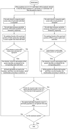
To improve the optimization performance of SSO algorithm, an improved strategy combining genetic algorithm, particle swarm algorithm, and SSO algorithm based on dual-population Evolution Mechanism is proposed in this paper. In the process of iteration, the SSO algorithm brings each individual of the shark population into the optimal position rapidly. Particle swarm algorithm has the same defect of local convergence as SSO algorithm due to its fixed foraging behavior. At the same time, the crossover and mutation of genetic algorithm can prevent the SSO algorithm based on evolutionary from stalling immediately when it falls into the local optimum, and it can cause certain disturbance and mutation, which can help the SSO algorithm to jump out of the local optimum dilemma. In addition, the composite angle cosine is used as the evaluation index and the parallel evolutionary mechanism of dual-population is adopted to prevent the population from being dominated by extreme individuals. The flowchart of improved shark smell optimization algorithm proposed in this paper is shown in Figure 4.
As can be seen form Figure 4, the dual-population strategy uses two populations (shark population and particle swarm ) to evolve at the same time, and compares the optimal individuals of the two populations, so as to break the equilibrium state in the population and to jump out of the local optimum.
In the optimization process, some generated particle may be beyond the boundary, the specific treated formula is described as follows,
where represents the sign of “if … then …” ; is the updated particle; is the maximum value of particle boundary; is the minimum value of particle boundary.
4. Experimental Simulation
4.1. Data and Parameters for Experimental Simulation
In this paper, the scenarios about Jinpu line No.1 and rail transit line No.12 in Dalian, China are selected as the research objects. Jinpu line No.1 is the intercity railway line that is 46.76 km long and has 11 stations in the initial stage, which extend from Jiuli light rail station to the terminal of Zhenxing road in Dalian under construction. Rail transit line No.12 is an urban rail transit line that is 40.38 km long and has 8 stations, which extend from Hekou station to terminal of Lvshun New Port. The simulation running line of scenario about Jinpu line No.1 is from the Jiuli to the 19th bureau, and the interval length between the above two station is 2.74 km. The running simulation line of scenario about rail transit line No.12 is from Lvshun New Port to Tieshan Town, and the interval length between the above two station is 2.94 km, with two long downhill and a long uphill ramps. The main parameters of the above scenarios are shown in Table 2 and Table 3, ramp parameters and velocity limit for automatic train operation are shown in Figure 5.
The calculation formula of traction characteristics is expressed as follows,
where is the instantaneous traction of vehicles, is the vehicle’s maximum traction, is the maximum traction power of the vehicle, is the switching velocity of the constant power zone and the reduced power zone, is the switching velocity of the traction starting region and constant torque region, and is the maximum design speed of the vehicle.
Simulation optimization results must satisfy the following conditions; the train instantaneous speed cannot surpass the speed limit, the train must finish the whole process, and the parking error is less than m. The improved shark smell optimization algorithm parameters are set as follows; the particle swarm size is 40, the weight coefficient is , the acceleration coefficients and are , crossover probability is 0.7, mutation probability is 0.09, selection probability is 0.5, the iteration number is 200, the shark population size is 40, the random number , , , , speed limit factor is 1.3, and the weight coefficient is . Setting parameters for the optimization algorithm is necessary to consider the convergence speed and optimization effect, such as population size and iteration number, with the increase of population size, the global search ability of the optimization algorithm will be enhanced, but the convergence speed will be reduced; similarly, with the increase of the number of iterations, the finding opportunity of optimal solution will be increase, and the more computing time and resource will be expend. The parameters characteristics and multiple experimental simulation results are taken into account for the above parameters setting. The multi-objective optimization parameters of the ATO scenario simulation of Jinpu line No.1 in Dalian are set as follows; the scheduled running time is ; ; ; ; the intrinsic weight factors ; and are, respectively, , , and ; the target demand vector is . The multi-objective optimization parameters of the ATO scenario simulation of rail transit line No.12 in Dalian are set as follows; the scheduled running time is 180 s, , , , the intrinsic weight factors , , and are, respectively, , , and , the target demand vector is .
4.2. Matlab/simulink Simulation Results for Automatic Train Operation Scenarios
According to the automatic train operation scenarios of rail transit line No.12 and Jinpu line No.1 in Dalian, China, the approximate optimal solutions are obtained by using the improved algorithm proposed in this paper, traditional improved shark smell optimization algorithm (chaotic shark smell optimization) [17] and traditional improved particle swarm optimization (dynamic multiple populations particle swarm optimization algorithm based on decomposition) [43], the above Matlab/simulink platform is chosen as a simulation platform. The specific configuration of the Matlab/simulink platform used in this paper is described as follow: the Matlab/simulink revision is Matlab GUI 2016b; the major computer configuration is “CPU Core i9-7920X @ 2.9 GHZ” and “Windows 10”. The specific Matlab/simulink optimization simulation results are shown in Figure 6 and Figure 7 and Table 4, Table 5, Table 6 and Table 7, and three different algorithms are recorded as ISSO, CSSO, and dMOPSO.
As can be seen in Table 4, Table 5, Table 6 and Table 7, the optimization solution obtained by the improved ISSO is superior to that of CSSO and dMOPSO, and three indexes of energy saving, punctuality, and comfort have been improved considerably. The ATO experiment simulation scenario for Jinpu line No.1 from Jiuli to the 19th bureau is a typical slope with ups and downs. It is necessary to keep the train at high speed before driving down the long down ramp. The ATO experiment simulation scenario for rail transit line No.12 from Lvshun New Port to Tieshan Town is in the hilly of Dalian Lvshunkou district, and the hilly region is the typical characteristics of Dalian. When the train is running in such a terrain, the control sequence should be concise. The train speeds up in the long down slope and slows down in the long up slope as much as possible, which can save energy and avoid turbulence. As can be seen from Figure 6a,b and Figure 7a,b ( the target velocity trajectory and control sequence ), the improved algorithm ISSO can obtain extremely simple control sequence and make the most of long down and up slopes, so as to obtain the target velocity trajectory as smooth as possible. As can be seen from Figure 6c,d and Figure 7c,d (the iterative convergence curves), the convergence rate of ISSO is faster than that of CSSO and dMOPSO. Even in the late iterations, ISSO has a strong ability of global convergence performance.
Compared with other comparison optimization algorithms, ISSO has several obvious advantages in matlab/simulation environment, as there is huge difference between matlab/simulation environment and actual scenario yet, the effectiveness of ISSO is necessary to further test and verify.
4.3. HILS Results for Automatic Train Operation Scenarios
Matlab/Simulink is a simulation technology that is completely separated from the real train operation environment. Therefore, some problems (such as real-time velocity sampled inaccurately, signal delay and packet loss in transmission, a certain degree of unstable in tracking control system, etc.) need to be considered in the actual control process and are cannot be truly reflected. To more effectively test the performance of the optimization algorithm in the actual train operation environment, dSPACE hardware-in-the-loop simulation (HILS) technology is adopted to write the verified optimization algorithm or control algorithm to the chip of the optimizer or controller. Compared to traditional simulation platform based on pure software environment, dSPACE HILS platforms contain the real on-board equipments, which can truly reflect the the real situation for automatic train operation. Due to the restriction of funds and experiment conditions, it is difficult to implement the corresponding actual automatic train operation experiment. Moreover, compared with real actual experiments, dSPACE HILS has the advantages of low experimental cost, implement easily, and high security protection of personal and equipment [33]. Therefore, HILS is highly valued by researchers and developers, abundant HILS-related products are researched, developed, and applied in various fields and numerous relative research results have been achieved [44,45]. The semi-physical simulation equipments in automatic train operation mainly include optimizer, controller, sensors, simulator, conditioning circuit, signal conditioning unit, and connector. The simulation topology diagram of automatic train operation HILS platform, the structure diagram for automatic train operation HILS, and the physical diagram of controller cabinet and simulation cabinet for automatic train operation HILS are shown in Figure 8 and Figure 9.
As can be seen from Figure 8, the Controller/Optimizer and its Service equipment make up the automatic train operation HILS platform, the Monitor serves as the monitoring center for human–computer interaction, and the Alarm set and Circuit breaker are the warning and protection center. Alarm set detects the working status of each HILS device in real-time, and the Circuit breaker is used to protect equipment by breaking when a certain kind of exception is detected. As can be seen from Figure 9, the automatic train operation HILS platform contains various actual hardware, and simulation hardware for automatic train operation. The “lower-layer control loop” based on controller and “upper-layer optimization loop” based on optimizer of HILS constitute the two independent communication systems, respectively, and there is a certain connection between the two loops. “Controller” is also named as traction control unit (TCU), which could provide control commands for corresponding equipments in real-time using a proper control algorithm in real-time, enable the the urban rail vehicle to track the ideal profile curve; “Optimizer” is also named as main processor unit (MPU), which could provide the velocity ideal trajectory profile (target speed curve of automatic train operation) for “lower-layer control loop” tracking control based on ’dSPACE emulator’. Second, the “dSPACE emulator”, “conditioning circuit”, “signal processing unit”, “sensors”, “connectors”, and so on are service equipments for ATO HILS: “dSPACE emulator” provides some correlative simulation environments for the automatic train operation HILS, the related models included such as accurate braking model, traction transformer model, running line model, velocity fluctuation model, etc.; “conditioning circuit” can regulate electrical waves properly for “Controller” appropriately; “signal processing unit” can regulate net signals properly for “Optimizer” appropriately; and the “sensors” and “connectors” are used to feed electrical waves and net signals back to the “Controller” and “Optimizer” in real-time. Third, the “DC power source”, “Converter system”, “Electric motor”, “Digital rheostat box”, and “Gear box” are simulation electric hardware equipments of in place of the actual: “DC power source” acts as the actual pantograph; “Converter system” transfer the electric energy from “DC power source” to “Electric motor” through a series of current-voltage conversion processes, it includes AC–DC converter, DC–AC converter, low-pass filters, etc.; “Electric motor” acts as the actual urban rail vehicle motors set; the capacity of simulation circuit loop is smaller than actual. In Figure 11, “train controller cabinet” and “train emulator cabinet” are the vital equipments for automatic train operation HILS, except controller and emulator, conditioning circuit, signal processing unit and corresponding switch groups are included.
Obviously, compared with these automatic train operation scenarios based on pure software (such as Matlab/simulink simulation), their identical scenarios based on HILS are closer to actual. Therefore, based on the same scenarios, tracking control algorithm and HILS platform, the comprehensive performance index for automatic train operation obtained by optimization algorithms could reflect the optimization performance of these algorithms effectively. To further verify the effectiveness of the algorithm, according to the automatic train operation scenarios of rail transit line No.12 and Jinpu line No.1 in Dalian, China, the approximate optimal solutions are obtained by using ISSO, CSSO, and dMOPSO, the above ATO HILS platform is chosen as simulation platform. The specific configuration of the ATO HILS platform used in this paper is described as follow: the Matlab/simulink revision is Matlab GUI 2016b; the major computer configuration is “CPU Core i9-7920X @ 2.9 GHZ” and “Windows 10”; the core chip of “Controller” and “Optimizer” is “TMS320F28335”; the simulation software of “dSPACE emulator” is dSPACE software(revision is control desk 6.1); the communication protocol of the ATO HILS is MVB (multifunction vehicle bus); the MPC (model predictive control) algorithm is adopted as tracking control algorithm; the three optimization algorithms (ISSO, CSSO, and dMOPSO) used are written in the kernel chip of “Optimizer” in “upper-layer optimization loop” for contrasting. The specific HILS optimization results obtained by “Optimizer” in “upper-layer optimization loop” are shown in Figure 10 and Figure 11 and Table 8, Table 9, Table 10 and Table 11.
In Figure 10a,b and Figure 11a,b (which is related to the optimization effect of automatic train operation process), the power is switched on, the pantograph is raised, the dSPACE simulator is in the working state (the “dSPACE” button is pressed), the human–computer interaction signal is normal (the “Design” button is green), and the circuit breaker is normally closed, which is in a normal optimization simulation state.
According to optimization simulation results of different algorithms in Table 8, Table 9, Table 10 and Table 11, compared with the traditional improved particle swarm optimization algorithm (dMOPSO) and traditional improved shark smell optimization algorithm (CSSO), the improved algorithm proposed in this paper (ISSO) has the obvious performance improvement effect, the three indexes of energy saving, punctuality and comfort of target velocity trajectory have been improved considerably; meanwhile, and the convergence evolution generations and computation time have been reduced considerably. As can be seen from Figure 10a,b and Figure 11a,b, the ideal target velocity trajectory obtained by ISSO was the smoothest, compared with the contrasted algorithms (CSSO and dMOPSO), ISSO obtained extremely simple control sequence and made use of the most of long down and up slopes sufficiently, it enables the train to reduce unnecessary traction and braking status and to make full use of coasting status as much as possible. As can be seen from Figure 10c,d and Figure 11c,d, compared with contrasted algorithms (CSSO and dMOPSO), the three optimization objective indexes and two unified goals obtained by ISSO have been improved to a considerable extent not only in the optimization effect but also in the computation efficiency.
Compared with the improving optimization effect of ATO target velocity trajectory optimization, improving the actual tracking control effect is more practical. The optimization effect calculation speed could estimate the performance of the ATO target velocity trajectory optimization algorithms, achievable difficulty for tracking control is also a significant evaluation index. To better verify the effectiveness of the ISSO, the “lower-layer control loop” is used to tracking control according to optimal target velocity trajectory generated by the “upper-layer control loop”. The MPC (model predictive control) algorithm has some its own advantages such as good performance in tracking precision, powerful robustness, fast tracking speed, etc. and widely in ATO traction system, so it is selected as tracking control algorithm in this paper. The specific HILS tracking control results obtained by “Controller” in “lower-layer control loop” are shown in Figure 12 and Figure 13 and Table 12 and Table 13.
In Figure 12 and Figure 13 (which relate to the tracking control effect of automatic train operation process according to optimization result), the power is switched on, the pantograph is raised, the dSPACE simulator is in the simulation state (the “dSPACE” button is pressed), the design parameters cannot be changed (the “Design” button is white), and the circuit breaker is normally closed, which is in a normal tracking control simulation state.
According to optimization simulation results of different algorithms from Table 12 and Table 13, compared with the traditional improved particle swarm optimization algorithm (dMOPSO) and traditional improved shark smell optimization algorithm (CSSO), the corresponding tracking control curve tracking the target velocity trajectory, obtained by improved algorithm proposed in this paper (ISSO), has the obvious performance improvement effect, the its three indexes of energy-saving, punctuality, and comfort have been improved considerably. As can be seen from Figure 12 and Figure 13, compared with the contrasted algorithms (CSSO and dMOPSO), the corresponding tracking control curve for ISSO has better tracking control effects. As can be seen from the enlarged areas of Figure 12 and Figure 13, the velocity fluctuation of the velocity distance trajectory curves corresponding to ISSO is weaker, because the target velocity trajectory obtained by ISSO was more ideal and tracking controlled easily in the automatic train operation simulation scenarios.
To verify that the improved algorithm (ISSO) in this paper has more superiorities, such as optimization effect, calculation speed, easily achievable in tracking control, etc., two scenarios about rail transit line No.12 and Jinpu line No.1 in Dalian, China are chosen as optimized objects for ISSO and some comparison algorithms, the corresponding optimization and tracking control results of matlab/simulation and hardware-in-the-loop simulation (HILS) as shown in Table 4, Table 5, Table 6, Table 7, Table 8, Table 9, Table 10, Table 11, Table 12 and Table 13 and Figure 5 and Figure 6, and Figure 10, Figure 11, Figure 12 and Figure 13. Obviously, compared with the contrasted algorithms (CSSO and dMOPSO), the corresponding optimization and tracking control results obtained by ISSO are more ideal. It is indicate that ISSO is a appropriate algorithm with powerful optimization capability, so as to solving practical automatic train operation more effectively.
5. Conclusions
Automatic train operation target velocity trajectory optimization is a very complex issue that needs to take into account multiple objectives, and the ideal optimization solution is not easy to be obtained. An improved multi-objective dual-population shark smell optimization algorithm using incorporated composite angle cosine for automatic train operation velocity trajectory optimization is proposed in this paper, and the specific advantages are described as follows.
For the multi-objective optimization problem, the evaluation index of the solution is very important. Nonetheless, the linear weighted target belongs to the common multi-objective unified target, and there is a problem that subjective parameters are selected blindly. In this paper, the multi-objective angle cosine is used as evaluation index, which can effectively avoid the blind selection of subjective parameters. To make the evaluation index more reasonable, on the basis of the preference information, the composite angle cosine which takes into account both the preference difference and the numerical difference is be used as the evaluation index of the solution in this paper.
Because the updating rules of velocities and positions in the SSO and PSO make all individuals close to the extreme individuals, after a long iteration, the extreme individuals will form a certain degree of dominance over the population, which makes it difficult to converge globally. First, the dual-population evolution mechanism is used to jump out of the local optimum. Second, to suppress the local convergence of optimization algorithm, it is necessary to determine accurately whether the individual aggregation occurs in shark population. In this paper, the fusion distance can be used to take into account the relativity and independence of speed and time, which can detect whether there is the phenomenon of individual aggregation preciously, so the local convergence is better suppressed. At the same time, this paper also introduces the dual-population collaborative optimization mechanism of SSO algorithm and particle swarm algorithm to further improve the optimization performance of the algorithm.
According to the the Matlab/simulink results and HILS results about automatic train operation scenarios, compared with the conventional improved shark smell optimization algorithm and the conventional improved particle swarm optimization algorithm, the improved algorithm (ISSO) proposed in this paper improves the calculation accuracy and optimization ability of the optimization algorithm to some extent, so that more ideal target velocity trajectory can be obtained. This clearly shows that ISSO have been improved to a considerable extent for the automatic train operation target velocity trajectory optimization not only in the pure software scenarios but also in the semi-physical scenarios. As the automatic train operation HILS is close to its actual experiment, the problem that the ISSO has worse improvement optimization effect in the actual than anticipatory could be avoid to certain extent.
Author Contributions
The work presented here was performed in collaboration among all authors. L.W. designed, analyzed, and wrote the paper, and completed the simulation experiment. X.W. guided the full text and provided simulation conditions. Z.S. conceived idea and involved simulation experiment. S.L. involved simulation experiment and analyzed the data. All authors have read and agree to the published version of the manuscript.
Funding
This research was funded by The Nature Science Foundation of China (grand number 51609033 and 61773049).
Conflicts of Interest
The authors declare no conflicts of interest.
Abbreviations
The following abbreviations are used in this manuscript:
| ATO | automatic train operation |
| HILS | hardware-in-the-loop simulation |
| ISSO | improved shark smell optimization |
| CSSO | chaotic shark smell optimization |
| dMOPSO | multi-objective particle swarm optimization based on decomposition |
References
- Wang, G.; Xiao, S.; Chen, X. Application of Genetic Algorithm in Automatic Train Operation. Wirel. Pers. Commun. 2018, 102, 1695–1704. [Google Scholar] [CrossRef]
- Tan, Z.; Lu, S.; Bao, K.; Zhang, S.; Wu, C.; Yang, J.; Xue, F. Adaptive Partial Train Speed Trajectory Optimization. Energies 2018, 11, 3302. [Google Scholar] [CrossRef] [Green Version]
- Gu, Q.; Tang, T.; Cao, F.; Song, Y. Energy-Efficient Train Operation in Urban Rail Transit Using Real-Time Traffic Information. IEEE Trans. Intell. Transp. Syst. 2014, 15, 1216–1233. [Google Scholar] [CrossRef]
- Bai, Y.; Ho, T.K.; Mao, B.; Ding, Y.; Chen, S. Energy-Efficient Locomotive Operation for Chinese Mainline Railways by Fuzzy Predictive Control. IEEE Trans. Intell. Transp. Syst. 2014, 15, 938–948. [Google Scholar] [CrossRef]
- Song, Y.; Song, W. A Novel Dual Speed-Curve Optimization Based Approach for Energy-Saving Operation of High-Speed Trains. IEEE Trans. Intell. Transp. Syst. 2016, 17, 1564–1575. [Google Scholar] [CrossRef]
- Domínguez, M.; Fernández-Cardador, A.; Cucala, A.P.; Pecharromán, R.R. Energy Savings in Metropolitan Railway Substations Through Regenerative Energy Recovery and Optimal Design of ATO Speed Profiles. IEEE Trans. Autom. Sci. Eng. 2012, 9, 496–504. [Google Scholar] [CrossRef]
- Shangguan, W.; Yan, X.; Cai, B.; Wang, J. Multiobjective Optimization for Train Speed Trajectory in CTCS High-Speed Railway With Hybrid Evolutionary Algorithm. IEEE Trans. Intell. Transp. Syst. 2015, 16, 2215–2225. [Google Scholar] [CrossRef]
- Huang, Y.; Yang, L.; Tang, T.; Cao, F.; Gao, Z. Saving Energy and Improving Service Quality: Bicriteria Train Scheduling in Urban Rail Transit Systems. IEEE Trans. Intell. Transp. Syst. 2016, 17, 3364–3379. [Google Scholar] [CrossRef]
- Fernandez-Rodriguez, A.; Fernández-Cardador, A.; Cucala, A.P.; Domínguez, M.; Gonsalves, T. Design of Robust and Energy-Efficient ATO Speed Profiles of Metropolitan Lines Considering Train Load Variations and Delays. IEEE Trans. Autom. Sci. Eng. 2015, 16, 2061–2071. [Google Scholar] [CrossRef] [Green Version]
- Bocharnikov, Y.V.; Tobias, A.M.; Roberts, C.; Hillmansen, S.; Goodman, C.J. Optimal driving strategy for traction energy saving on DC suburban railways. IET Electr. Power Appl. 2012, 181, 51–62. [Google Scholar] [CrossRef]
- Gu, Q.; Tang, T.; Ma, F. Energy-Efficient Train Tracking Operation Based on Multiple Optimization Models. IEEE Trans. Intell. Transp. Syst. 2016, 17, 882–892. [Google Scholar] [CrossRef]
- Zhou, Y.; Tao, X. Robust Safety Monitoring and Synergistic Operation Planning Between Time and Energy-Efficient Movements of High-Speed Trains Based on MPC. IEEE Access 2018, 6, 17377–17390. [Google Scholar] [CrossRef]
- Kunimatsu, T.; Hirai, C.; Tomii, N. Train timetable evaluation from the viewpoint of passengers by microsimulation of train operation and passenger flow. Electr. Eng. Jpn. 2012, 181, 51–62. [Google Scholar] [CrossRef]
- Abedinia, O.; Amjady, N.; Ghasemi, A. A new metaheuristic algorithm based on shark smell optimization. Complexity 2014, 21, 97–116. [Google Scholar] [CrossRef]
- Gnanasekaran, N.; Chandramohan, S.; Kumar, P.S.; Imran, A.M. Optimal placement of capacitors in radial distribution system using shark smell optimization algorithm. Ain Shams Eng. J. 2016, 7, 907–916. [Google Scholar] [CrossRef] [Green Version]
- Ahmadigorji, M.; Amjady, N. A multiyear DG-incorporated framework for expansion planning of distribution networks using binary chaotic shark smell optimization algorithm. Energy 2016, 102, 199–215. [Google Scholar] [CrossRef]
- Abedinia, O.; Amjady, N. Short-term wind power prediction based on Hybrid Neural Network and chaotic shark smell optimization. Int. J. Precis. Eng. Manuf.-Green Technol. 2017, 5, 13062–13076. [Google Scholar] [CrossRef] [Green Version]
- Sicre, C.; Asunción, P.C.; Antonio, F.; Lukaszewicz, P. Modeling and optimizing energy-efficient manual driving on high-speed lines. IEEJ Trans. Electr. Electron. Eng. 2012, 7, 633–640. [Google Scholar] [CrossRef]
- Jiateng, Y.; Chen, D.; Li, L. Intelligent Train Operation Algorithms for Subway by Expert System and Reinforcement Learning. IEEE Trans. Intell. Transp. Syst. 2014, 15, 2561–2571. [Google Scholar]
- Cheng, R.; Yu, W.; Song, Y.; Chen, D.; Ma, X.; Cheng, Y. Intelligent Safe Driving Methods Based on Hybrid Automata and Ensemble CART Algorithms for Multihigh-Speed Trains. IEEE Trans. Cybern. 2019, 49, 3816–3826. [Google Scholar] [CrossRef]
- Meng, J.; Xu, R.; Li, D.; Chen, X. Combining the Matter-Element Model With the Associated Function of Performance Indices for Automatic Train Operation Algorithm. IEEE Trans. Intell. Transp. Syst. 2019, 20, 253–263. [Google Scholar] [CrossRef]
- Ma, J.; Fan, Z.; Jiang, Y.; Mao, J. An optimization approach to multiperson decision-making based on different formats of preference information. IEEE Trans. Syst. Man, Cybern. Part A Syst. Hum. 2006, 36, 876–889. [Google Scholar]
- Kaddani, S.; Vanderpooten, D.; Vanpeperstraete, J.M.; Aissi, H. Weighted sum model with partial preference information: Application to Multi-Objective Optimization. Eur. J. Oper. Res. 2017, 26, 665–679. [Google Scholar] [CrossRef]
- Nelyubin, A.P.; Podinovski, V.V. Multicriteria choice based on criteria importance methods with uncertain preference information. Comput. Math. Math. Phys. 2016, 57, 1475–1483. [Google Scholar] [CrossRef]
- Mayet, C.; Delarue, P.; Bouscayrol, A.; Chattot, E. Hardware-In-the-Loop Simulation of Traction Power Supply for Power Flows Analysis of Multi-Train Subway Lines. IEEE Trans. Veh. Technol. 2017, 66, 5564–5571. [Google Scholar] [CrossRef]
- De Farias, A.B.C.; Rodrigues, R.S.; Murilo, A.; Lopes, R.V.; Avila, S. Low-Cost Hardware-in-the-Loop Platform for Embedded Control Strategies Simulation. IEEE Access 2019, 7, 111499–111512. [Google Scholar] [CrossRef]
- Terwiesch, P.; Keller, T.; Scheiben, E. Rail vehicle control system integration testing using digital hardware-in-the-loop simulation. IEEE Trans. Control Syst. Technol. 1999, 7, 352–362. [Google Scholar] [CrossRef] [Green Version]
- Yang, X.; Yang, C.; Peng, T.; Liu, B.; Gui, W. Hardware-in-the-Loop Fault Injection for Traction Control System. IEEE J. Emerg. Sel. Top. Power Electron. 2018, 6, 696–706. [Google Scholar] [CrossRef]
- Zhang, H.; Zhang, Y.; Yin, C. Hardware-in-the-Loop Simulation of Robust Mode Transition Control for a Series-Parallel Hybrid Electric Vehicle. IEEE Trans. Veh. Technol. 2016, 63, 1059–1069. [Google Scholar] [CrossRef]
- Abdelrahman, A.; Algarny, K.; Youssef, M. A Novel Platform for Powertrain Modeling of Electric Cars With Experimental Validation Using Real-Time Hardware in the Loop (HIL): A Case Study of GM Second Generation Chevrolet Volt. IEEE Trans. Power Electron. 2018, 33, 9762–9771. [Google Scholar] [CrossRef]
- Cheng, J.; Howlett, P. Application of critical velocities to the minimisation of fuel consumption in the control of trains. Automatica 1992, 28, 165–169. [Google Scholar] [CrossRef]
- Wang, P.; Goverde, R.M.P. Multiple-phase train trajectory optimization with signalling and operational constraints. Transp. Res. Part C Emerg. Technol. 2016, 69, 255–275. [Google Scholar] [CrossRef]
- Chen, D.; Chen, R.; Li, Y.; Tang, T. Online Learning Algorithms for Train Automatic Stop Control Using Precise Location Data of Balises. IEEE Trans. Intell. Transp. Syst. 2013, 14, 1526–1535. [Google Scholar] [CrossRef]
- Howlett, P.; Cheng, J. Optimal driving strategies for a train on a track with continuously varying gradient. J. Aust. Math. Soc. 1997, 38, 388–410. [Google Scholar] [CrossRef] [Green Version]
- Liang, Y.; Liu, H.; Qian, C. A Modified Genetic Algorithm for Multi-Objective Optimization on Running Curve of Automatic Train Operation System Using Penalty Function Method. Int. J. Intell. Transp. Syst. Res. 2019, 17, 74–87. [Google Scholar] [CrossRef]
- Cheng, H.; Huang, W.; Zhou, Q.; Cai, J. Solving fuzzy multi-objective linear programming problems using deviation degree measures and weighted max-min method. Appl. Math. Model. 2013, 37, 6855–6869. [Google Scholar] [CrossRef]
- Fan, Z.; Liu, Z.; Li, X.; Gao, Z.; Su, X. Cross-study validation and combined analysis of microarray data for cancer using vector cosine angle method. In Proceedings of the 2005 IEEE Engineering in Medicine and Biology 27th Annual Conference, Shanghai, China, 17–18 January 2006; pp. 4810–4813. [Google Scholar]
- Xu, Z. Multiple-attribute group decision-making with different formats of preference information on attributes. IEEE Trans. Syst. Man Cybern. Part B 2007, 37, 1500–1511. [Google Scholar]
- Liu, G.; Wang, X. Fault diagnosis of diesel engine based on fusion distance calculation. In Proceedings of the Advanced Information Management, Communicates, Electronic and Automation Control Conference, Xi’an, China, 3–5 October 2016; pp. 1621–1627. [Google Scholar]
- Zhou, J.; Wang, C.; Li, Y.; Wang, P.; Li, C.; Lu, P.; Mo, L. A multi-objective multi-population ant colony optimization for economic emission dispatch considering power system security. Appl. Math. Model. 2017, 45, 684–704. [Google Scholar] [CrossRef]
- Park, T.; Ryu, K.R. A Dual-Population Genetic Algorithm for Adaptive Diversity Control. IEEE Trans. Evol. Comput. 2010, 14, 865–884. [Google Scholar] [CrossRef]
- Xu, M.; You, X.; Liu, S. A novel Heuristic communication Heterogeneous dual population Ant Colony Optimization algorithm. IEEE Access 2017, 5, 18506–18515. [Google Scholar] [CrossRef]
- Peng, H.; Li, R.; Cao, L.; Li, L. Multiple Swarms Multi-Objective Particle Swarm Optimization Based on Decomposition. Procedia Eng. 2011, 15, 3371–3375. [Google Scholar]
- Hasanzadeh, A.; Edrington, C.S.; Stroupe, N.; Bevis, T. Real-Time Emulation of a High-Speed Microturbine Permanent-Magnet Synchronous Generator Using Multiplatform Hardware-in-the-Loop Realization. IEEE Trans. Ind. Electron. 2014, 61, 3109–3118. [Google Scholar] [CrossRef]
- Nariman, R.T.; Venkata, D. A General Framework for FPGA-Based Real-Time Emulation of Electrical Machines for HIL Applications. IEEE Trans. Ind. Electron. 2015, 62, 2041–2053. [Google Scholar]
Figure 1.
The angle cosine diagram of the solution vector and the target demand vector.

Figure 2.
Schematic diagram of the preference phenomenon classification and the preference angle.

Figure 3.
The schematic diagram of the compound angle cosine.

Figure 4.
The flowchart of improved shark smell optimization algorithm proposed in this paper.

Figure 5.
The ramp parameters and the speed limit of experiment simulation for two ATO scenarios. (a) Jinpu line No.1 in Dalian scenario. (b) rail transit line No.12 in Dalian scenario.
Figure 5.
The ramp parameters and the speed limit of experiment simulation for two ATO scenarios. (a) Jinpu line No.1 in Dalian scenario. (b) rail transit line No.12 in Dalian scenario.

Figure 6.
The Matlab/Simulink optimization curves of different algorithms for Jinpu line No.1 in Dalian scenario. (a) Jinpu line No.1 in Dalian scenario. (a) Target velocity trajectory profiles. (b) Operating condition distance curves. (c) Iterative convergence curves of each optimization objectives. (d) Iterative convergence curves of unified goals.

Figure 7.
The Matlab/simulink optimization curves of different algorithms for rail transit line No.12 in Dalian scenario. (a) Target velocity trajectory profiles. (b) Operating condition distance curves. (c) Iterative convergence curves of each optimization objectives. (d) Iterative convergence curves of unified goals.

Figure 8.
The simulation topology diagram of automatic train operation hardware-in-the-loop simulation (HILS) platform.
Figure 8.
The simulation topology diagram of automatic train operation hardware-in-the-loop simulation (HILS) platform.

Figure 9.
The structure diagram for automatic train operation HILS.

Figure 10.
The HILS optimization curves of different algorithms for Jinpu line No.1 in Dalian scenario. (a) Target velocity trajectory profiles. (b) Operating condition distance curves. (c) Iterative convergence curves of each optimization objectives. (d) Iterative convergence curves of unified goals.

Figure 11.
The HILS optimization curves of different algorithms for rail transit line No.12 in Dalian scenario. (a) Target velocity trajectory profiles. (b) Operating condition distance curves. (c) Iterative convergence curves of each optimization objectives. (d) Iterative convergence curves of unified goals.

Figure 12.
The HILS tracking control curves of different algorithms for Jinpu line No.1 in Dalian scenario.
Figure 12.
The HILS tracking control curves of different algorithms for Jinpu line No.1 in Dalian scenario.

Figure 13.
The HILS tracking control curves of different algorithms for rail transit line No.12 in Dalian scenario.
Figure 13.
The HILS tracking control curves of different algorithms for rail transit line No.12 in Dalian scenario.


Table 1.
The preference categories circumstances in automatic train operation velocity trajectory optimization.
Table 1.
The preference categories circumstances in automatic train operation velocity trajectory optimization.
| Categories & Valuation Level | Prefect | Qualified | Unqualified |
|---|---|---|---|
| Energy Consumption | |||
| Comfort level | |||
| Time error |
Table 2.
The main parameters of the scenario about Jinpu line No.1 in Dalian.
| Parameter Name | Parameter Characteristics |
|---|---|
| Train weight (t) | 209 |
| Maximum running speed (km/h) | 80 |
| Formation plan | 2 motor 2 trail |
| Mean starting acceleration (m/s | (0∼35 km/h) ≥ 1.0 |
| Mean acceleration (m/s | (0∼80 km/h) ≥ 0.6 |
| Mean braking deceleration (m/s | (80∼0 km/h) ≥ 1.0 |
Table 3.
The main parameters of the scenario about rail transit line No.12 in Dalian.
| Parameter Name | Parameter Characteristics |
|---|---|
| Train weight (t) | 211 |
| Maximum running speed (km/h) | 80 |
| Formation plan | 2 motor 2 trail |
| Mean starting acceleration (m/s | (0∼35 km/h) ≥ 1.0 |
| Mean acceleration (m/s | (0∼80 km/h) ≥ 0.6 |
| Mean braking deceleration (m/s | (80∼0 km/h) ≥ 1.0 |
Table 4.
The Matlab/simulink optimization results of different algorithms for Jinpu line No.1 in Dalian scenario.
Table 4.
The Matlab/simulink optimization results of different algorithms for Jinpu line No.1 in Dalian scenario.
| Algorithm | Energy Consumption | Actual Time | Comfort Level |
|---|---|---|---|
| ISSO | 104,739 KJ | 177.0153 s | 6.392 m/skm |
| CSSO | 110,910 KJ | 177.0387 s | 7.142 m/skm |
| dMOPSO | 116,157 KJ | 177.0924 s | 7.655 m/skm |
Table 5.
The Matlab/simulink evaluate results of different algorithms for Jinpu line No.1 in Dalian scenario.
Table 5.
The Matlab/simulink evaluate results of different algorithms for Jinpu line No.1 in Dalian scenario.
| Algorithm | Angle Cosine | Linear Weighted Target | Computation Time | Convergence Evolution Generations |
|---|---|---|---|---|
| ISSO | 0.9446 | 0.1498 | 1722 s | 96 |
| CSSO | 0.8760 | 0.2554 | 1833 s | 126 |
| dMOPSO | 0.7129 | 0.3602 | 2585 s | 137 |
Table 6.
The Matlab/simulink optimization results of different algorithms for rail transit line No.12 in Dalian scenario.
Table 6.
The Matlab/simulink optimization results of different algorithms for rail transit line No.12 in Dalian scenario.
| Algorithm | Energy Consumption | Actual Time | Comfort Level |
|---|---|---|---|
| ISSO | 98,749 KJ | 180.0139 s | 5.638 m/skm |
| CSSO | 107,154 KJ | 180.0394 s | 6.537 m/skm |
| dMOPSO | 109,469 KJ | 180.0878 s | 7.408 m/skm |
Table 7.
The HILS evaluation of the results of different algorithms for Jinpu line No.1 in Dalian scenario.
Table 7.
The HILS evaluation of the results of different algorithms for Jinpu line No.1 in Dalian scenario.
| Algorithm | Angle Cosine | Linear Weighted Target | Computation Time | Convergence Evolution Generations |
|---|---|---|---|---|
| ISSO | 0.9566 | 0.1776 | 4476 s | 109 |
| CSSO | 0.8711 | 0.2759 | 4962 s | 130 |
| dMOPSO | 0.8542 | 0.3501 | 7031 s | 146 |
Table 8.
The Matlab/simulink evaluate results of different algorithms for rail transit line No.12 in Dalian scenario.
Table 8.
The Matlab/simulink evaluate results of different algorithms for rail transit line No.12 in Dalian scenario.
| Algorithm | Angle Cosine | Linear Weighted Target | Computation Time | Convergence Evolution Generations |
|---|---|---|---|---|
| ISSO | 0.9722 | 0.2205 | 1935 s | 114 |
| CSSO | 0.8829 | 0.3571 | 2194 s | 134 |
| dMOPSO | 0.7564 | 0.4547 | 2896 s | 119 |
Table 9.
The HILS optimization results of different algorithms for Jinpu line No.1 in Dalian scenario.
Table 9.
The HILS optimization results of different algorithms for Jinpu line No.1 in Dalian scenario.
| Algorithm | Energy Consumption | Actual Time | Comfort Level |
|---|---|---|---|
| ISSO | 106,741 KJ | 177.0135 s | 6.824 m/skm |
| CSSO | 115,245 KJ | 177.0430 s | 7.508 m/skm |
| dMOPSO | 119,569 KJ | 177.0428 s | 8.029 m/skm |
Table 10.
The HILS optimization results of different algorithms for rail transit line No.12 in Dalian scenario.
Table 10.
The HILS optimization results of different algorithms for rail transit line No.12 in Dalian scenario.
| Algorithm | Energy Consumption | Actual Time | Comfort Level |
|---|---|---|---|
| ISSO | 98,524 KJ | 180.0194 s | 5.712 m/skm |
| CSSO | 110,524 KJ | 180.0294 s | 7.194 m/skm |
| dMOPSO | 114,755 KJ | 180.0921 s | 7.844 m/skm |
Table 11.
The HILS evaluate results of different algorithms for rail transit line No.12 in Dalian scenario.
Table 11.
The HILS evaluate results of different algorithms for rail transit line No.12 in Dalian scenario.
| Algorithm | Angle Cosine | Linear Weighted Target | Computation Time | Convergence Evolution Generations |
|---|---|---|---|---|
| ISSO | 0.9515 | 0.2260 | 4365 s | 99 |
| CSSO | 0.8441 | 0.4009 | 5027 s | 126 |
| dMOPSO | 0.7682 | 0.5251 | 7885 s | 133 |
Table 12.
The HILS tracking control results of different algorithms for Jinpu line No.1 in Dalian scenario.
Table 12.
The HILS tracking control results of different algorithms for Jinpu line No.1 in Dalian scenario.
| Algorithm | Energy Consumption | Actual Time | Comfort Level |
|---|---|---|---|
| ISSO | 117,259 KJ | 177.0351 s | 32.947 m/skm |
| CSSO | 134,845 KJ | 177.1045 s | 41.859 m/skm |
| dMOPSO | 138,672 KJ | 177.1282 s | 43.578 m/skm |
Table 13.
The HILS tracking control results of different algorithms for rail transit line No.12 in Dalian scenario.
Table 13.
The HILS tracking control results of different algorithms for rail transit line No.12 in Dalian scenario.
| Algorithm | Energy Consumption | Actual Time | Comfort Level |
|---|---|---|---|
| ISSO | 115,168 KJ | 180.0397 s | 37.027 m/skm |
| CSSO | 128,122 KJ | 180.0823 s | 44.254 m/skm |
| dMOPSO | 137,485 KJ | 180.1465 s | 47.966 m/skm |
© 2020 by the authors. Licensee MDPI, Basel, Switzerland. This article is an open access article distributed under the terms and conditions of the Creative Commons Attribution (CC BY) license (http://creativecommons.org/licenses/by/4.0/).
Share and Cite
MDPI and ACS Style
Wang, L.; Wang, X.; Sheng, Z.; Lu, S. Multi-Objective Shark Smell Optimization Algorithm Using Incorporated Composite Angle Cosine for Automatic Train Operation. Energies 2020, 13, 714. https://doi.org/10.3390/en13030714
AMA Style
Wang L, Wang X, Sheng Z, Lu S. Multi-Objective Shark Smell Optimization Algorithm Using Incorporated Composite Angle Cosine for Automatic Train Operation. Energies. 2020; 13(3):714. https://doi.org/10.3390/en13030714
Chicago/Turabian StyleWang, Longda, Xingcheng Wang, Zhao Sheng, and Senkui Lu. 2020. "Multi-Objective Shark Smell Optimization Algorithm Using Incorporated Composite Angle Cosine for Automatic Train Operation" Energies 13, no. 3: 714. https://doi.org/10.3390/en13030714
Note that from the first issue of 2016, this journal uses article numbers instead of page numbers. See further details here.