Abstract
Risk-based redispatch optimization is proposed as a methodology to support the Transmission System Operator (TSO) with preventive remedial actions obtained by extending the security-constrained unit commitment/economic dispatch with constraints resulting from the risk assessed for the power system. Although being heuristic, the methodology is based on comprehensive dynamic security assessment as time-domain simulations are used, allowing to express the degree of all types of instabilities, e.g., caused by contingencies, in monetary terms. Therefore, the risk is assessed as the expected value of the cost incurred by the TSO. Such an approach forms a new pathway to including risk in planning procedures already used by TSOs. Results obtained for the IEEE39 dynamic power system, with costs assigned to load shedding and generator tripping due to single transmission lines short-circuits, are shown as a reference case.
1. Introduction
What the authors of this paper consider as a challenge for power system planners is the process of switching from security assessment that is deterministic and independent from the current weather conditions to one utilizing an adaptive stochastic approach. In this paper, a risk-based solution is proposed, in particular one that could allow power system planners to consider the influence of weather conditions on the probability of contingencies.
To date, the most accepted security procedure is based on the N-1 criterion, which when integrated with the security-constrained unit commitment/economic dispatch or security-constrained optimal power flow methods (SC UC/ED or SC OPF, respectively) allows one to ensure that the system parameters remain within safety limits after removing one of its elements. The aforementioned methods are understood as follows:
- SC UC results with a list of committed units taking into account all inter-temporal and network constraints, as well as the N-1 security criterion;
- SC ED provides operating points for units with respect to those constraints;
- SC OPF does not take into account inter-temporal constraints while the network constraints and the N-1 criterion are still included.
However, apart from being deterministic, those methods apply only to steady-state equations and therefore skip the power systems dynamic phenomena related to frequency, voltage and angle stability. On the other hand, the main concept behind the proposed method is that preventive remedial actions are designed in order to reduce the risk associated with phenomena caused by generators trips resulting from contingencies. Here, such reduction is performed using the active power redispatch based on an iterative process including the SC UC/ED tool, which is coupled with risk assessment utilizing an adaptive stochastic approach. Such a methodology of risk assessment was thoroughly described and extended in a former paper by the authors [1].
The aforementioned iterative coupling was proposed as it is not possible to combine the dynamic simulations with SC UC/ED in one optimization problem without simplifications, e.g., acquiring separate optimization tools handling transient, frequency, and voltage phenomena independently. Hence, the motivation of this paper is to propose an iterative optimization tool as a solution, especially if the SC UC/ED tool is already owned by a TSO. The broader context follows the state-of-the-art review.
1.1. Literature Review
Several interesting approaches to extending the SC UC/ED and SC OPF with constraints based on transient stability assessment (TSA) may be found in the literature, however, they differ with respect to many criteria. First of all the way of incorporating rotor dynamics into the linear optimization problem spans from using trapezoidal rule [2,3] or Taylor series expansion [4] (to convert differential equations into algebraic ones) to involving direct (or direct-temporal) TSA methods like single-machine equivalent (SIME) [3,5,6,7] or the transient energy function (TEF) [8,9,10,11]. These methods are used to rank the synchronous machines by their stability margin (or its sensitivity to generation changes) with respect to a considered set of contingencies, however, the critical clearing time (CCT) was used for ranking as well [12]. Secondly, the procedure of finding the amount of power to be shifted from the least stable generators could be based on the identified energy margins, inertia constants [11], values of the rotor speed at the fault clearing time [9] or the power angle trajectory sensitivity [13,14,15]. In most cases, the power shifting was performed in small steps within an iterative procedure. Hence, the final dispatch was obtained after several iterations of adjusting the constraints for OPF, solving it and repeating the transient stability assessment process, until the desired value of the stability margin or the CCT was found. However, more sophisticated approaches to solving the constrained OPF problem were also proposed to find the most stable dispatch—they included particle swarm optimization, genetic algorithms and neural networks [12,16]. Lastly, the details of the dynamic models used to perform time-domain simulations (TDS) were found to be of importance. In particular, using dynamic instead of static load models [6] or 4th order generator models (along with excitation systems and automatic voltage regulator (AVR) models instead of constant voltage behind a transient reactance) [7] was shown to improve the stability of the resulting dispatch.
1.2. Scope of This Paper
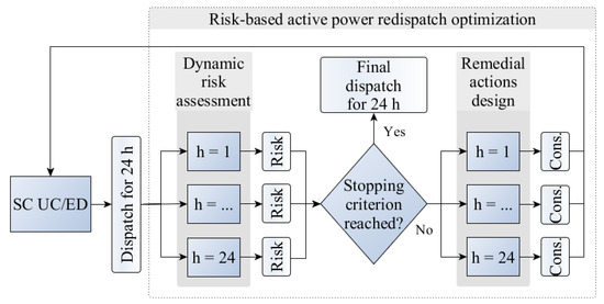
The general scheme of the redispatch optimization proposed in this paper is shown in Figure 1. Its basic concept is similar to those described above [2,3,4,5,6,7,8,9,10,11,12,13,14,15], but there are three major differences. First of all, going beyond TSA towards a more comprehensive dynamic security assessment is considered here, where not only transient rotor angle but also frequency and voltage instabilities may be tackled—by applying proper dynamic models [7]. Secondly, the procedure is based on interactions between a standard SC UC/ED tool and the proposed risk-based redispatch optimization, which includes two processes, namely the dynamic risk assessment and the remedial action design (shown as solid gray boxes in Figure 1). With the SC UC/ED tool considered as providing operating points for 24 h, the dynamic risk assessment results in Risk values assessed for each of them. Afterwards, in case the risk-based stopping criterion is met, the dispatch is considered as final with no more iterations required. Otherwise, the remedial actions are designed within the second process resulting in Cons.—modifications of generators units constraints present in SC UC/ED. Hence, all the SC UC/ED hourly dispatches obtained within the next iterations will satisfy both the risk-based security constraints and the inter-temporal constraints of the units. Considering the above, the proposed method does not replace and does not require any modifications of the SC UC/ED tools already used by TSOs (e.g., for operational planning), but is used only to provide its input. This input is used to adjust the generator unit constraints for the dispatch optimization problem to assure not only static but also dynamic security. Lastly, the proposed risk-based redispatch optimization module uses a stochastic approach to identify remedial actions that are based on the value of the assessed risk (being a function of probability and cost) and aimed to decrease that risk until a specified stopping criterion is reached.
The paper is organized as follows. The methodology of obtaining the risk assessment and remedial actions is described in Section 2. The results for the IEEE39 power system are presented and discussed in Section 3. The paper is concluded by summarizing the results and considering further extensions of the proposed method.
2. Theoretical Framework
The SC UC/ED process used within the approach shown in Figure 1 is considered as a self-contained standard tool used by TSOs to obtain the operating points (e.g., for 24 h), based on the DC or AC power flow solutions. However, it is assumed to fulfill several criteria including those assuring static security (e.g., withstanding N-k outages) or other tuned to meet particular requirements of the TSO. The purpose of the two main components of the presented generation redispatch optimization method, namely the processes of dynamic risk assessment and remedial action design, is to be coupled with the SC UC/ED only by adjusting its constraints. The details of that coupling, including the two main components used in the iterative process starting from the output of the SC UC/ED tool, are described in the following subsections.
2.1. Dynamic Risk Assessment
Each hourly dispatch resulting from SC UC/ED is used in an independent dynamic risk assessment process as presented in Figure 2. It comprises three elements, i.e., probability estimation, cost calculation and risk assessment. The probabilities may be obtained with the help of historical data or adjusted according to weather forecasts. Within the cost calculation process, the Dynamic Security Assessment (DSA) is used—the operating points of synchronous generators are obtained from SC UC/ED and used as initial conditions for time-domain simulations (TDS) [2,12,13,14,15,16]. The cost is obtained based on the events taking place during TDS after the inception of each fault (e.g., a short-circuit) initiating the considered contingency—an example of the cost calculation procedure is provided in Appendix A.
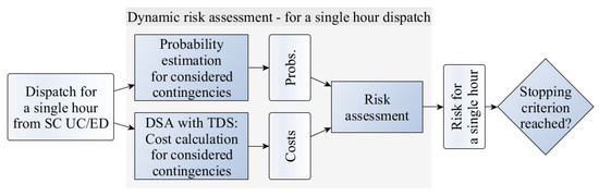
Figure 2.
Detailed scheme of the dynamic risk assessment process for a single hour dispatch resulting from the SC UC/ED solution.
Afterwards, the value of the risk is obtained in the simplest form as described by (1):
where R—the total risk of the system, —risk related to contingency C, —the probability and —the cost assigned to contingency C.
2.2. Remedial Actions Design
The process from Figure 2 is continued once the selected stopping criterion is not met, even for one of the considered hourly dispatches. In particular, the remedial actions (RA) are prepared based on the assessed risk—this continuation is depicted in Figure 3, again, independently for each hourly system state. With the variety of consequences that might be reflected by that risk value in general, e.g., reactions of protection relays due to violations of thermal limits, rotor angle, and frequency and voltage instabilities, the remedial actions may be designed to involve redispatching active and reactive power, capacitors, energy storage systems, etc. For the purposes of our research, preventive remedial actions are considered and based on adjusting the constraints for active power generation levels of synchronous machines in SC UC/ED. The aim of such remedial actions is to prevent the synchronous machines from being tripped by allowing them to withstand dynamic instabilities caused by the simulated faults. This aim is achieved by lowering generation levels of the least stable machines, preventing them from losing synchronism after short-circuits with longer clearing times [17].
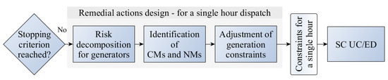
Figure 3.
Detailed scheme of the remedial actions design process for a single hour result of the dynamic risk assessment from Figure 2.
2.3. Stopping Criteria
In between the dynamic risk assessment and the remedial actions design, this risk values R are used to verify the stopping criterion and assess whether remedial actions are necessary. In the first approach, a threshold-based stopping criterion similar to the ones described in the literature [2,3,4,5,6,7,8,9,10,11,12,13,14,15] was used and its aim was to allow stabilizing the system against credible contingencies. It was defined by the following inequality (2):
To test the convergence of the proposed method, the was used to obtain the results (see Section 3). The second approach was introduced in which the process is stopped after reaching the minimal value of the sum of the operating cost of generating units (resulting from SC UC/ED) and the risk R related to dynamic security of the system—this is defined by (3):
2.4. Redispatch Process
The risk R assessed with the help of (1) is a global value describing the whole system in the state provided by each hourly dispatch from SC UC/ED. However, we decompose it to every synchronous generator and identify the critical (the least stable ones) and non-critical machines (CMs and NMs, respectively). Similar identification is used in many approaches listed in Section 1, including those utilizing SIME [3,5,6,7] or TEF [10,11] methods. It serves the purpose of conducting the redispatch by shifting the active power from CMs to NMs. Nevertheless, only in this approach CMs and NMs are identified basing on the dynamic risk. To perform the redispatch, we start with distributing the risk contribution (from (1)) of every contingency C between the generators tripped due to C—those generators form the set . If there is only one generator in , the risk value is assigned to it directly. However, in cases with many generators tripped after a contingency, the value of risk is split into all those generators proportionally to —the active power supplied by each generator G. This is done according to the risk defined for every tripped generator:
where is the current active power generated by machines in .
Afterwards, the risk values resulting from all considered contingencies are assigned to particular generators according to:
This, in turn, allows us to perform the aforementioned identification of CMs and NMs, keeping in mind the following—only a fraction of the power from CMs is shifted to NMs in one iteration of the process from Figure 1 (alike in [7,11]). Hence, the final result of the redispatch is reached gradually with relatively small steps (i.e., ) and what follows is the absolute value of power to be shifted from CMs to NMs:
What is also important is the power margin of NMs (depending on the current operating points and maximal generations powers of particular generators):
which should allow the shifting and therefore the inequality (8) should be satisfied:
Hence, if the initial set of machines with does not have the proper power margin, we continue to extend this set by successively adding generators with the smallest value of , until (8) is satisfied. The power to be shifted from each of the CMs taking into account the step value and the generators risk is expressed as:
which is used to adjust the constraints of CMs in the following way:
The generation limits of NMs are not modified, whereas the values from (10) go back as input to the SC UC/ED process in order to modify the constraints for CMs for each particular hour. There the preventive remedial actions are applied for all synchronous generators, as the SC UC/ED procedure joins the resulting constraints with the inter-temporal ones (e.g., based on generators ramp rates) coupling the generation levels for the whole set of 24 hours. Hence, the next iteration is started with a new daily dispatch (sets of for each hour) and the process continues until reaching the desired stopping criterion.
3. Results
This section presents the results of adapting the iterative method from Figure 1 to the IEEE39 power system for the purpose of obtaining dynamically secure operating points, with only one hourly dispatch chosen for simplicity. However, the results were obtained for two scenarios, namely the SC OPF and OPF (in AC versions). The former is more secure as it satisfies the static N-1 criterion, whereas the latter is profitable from both an economical and computational perspective. Moreover, we performed the sensitivity analysis with respect to several values of the iteration step for both dispatch scenarios. First of all, we extended the IEEE39 model with 10 additional lines which allowed us to improve the systems connectivity and hence reliability. Afterwards, we prepared the values of failure probability for each kilometer of the line basing on the mean time to repair and transmission lines failure frequency [18,19] published by PSE—the Polish TSO [20].
The data describing all 10 generators in IEEE39 are collected in Table 1, however, the generator from bus 30 is considered as an equivalent of an interconnection with the power supply held constant on the level of 1045 MW. The other 9 generators were modeled as synchronous machines, with . The variable costs were selected by a simplified matching the types of generators included in the model with the costs expected in Poland.

Table 1.
The data sheet on generators in IEEE39 with the initial operating points for SC OPF and OPF scenarios.
The initial operating points were supplied to the TDS and the process from Figure 2 was started with the N-1 contingencies simulated as 3-phase short-circuits. They were applied in 44 transmission lines (shown with solid lines in Figure 4), all of which were equipped with a distance impedance protection relay, which cleared the fault after 150 ms. As we mentioned in Section 2, the risk was calculated by taking into account the events of tripping the generators by out-of-step protection relays included in the dynamic model. Moreover, the load shed by under-frequency protection relays was also included, which gave us the opportunity of enhancing the assessment of transient rotor angle instabilities by additional assessment of the frequency stability. Furthermore, we equipped our IEEE39 dynamic model with models of overcurrent protection relays, the actions of which could also be responsible for disconnecting bus loads resulting in additional costs. In order to include the actions of all aforementioned protection relays, the TDS were performed until achieving the steady-state.
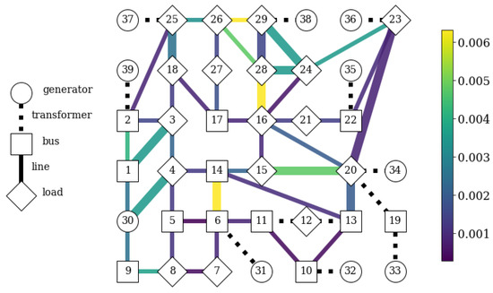
Figure 4.
The schematic graph of the IEEE39 network with two legends: left showing symbols used in the graph and the right with N-1 fault probabilities obtained by utilizing the historical data published by PSE (Polish TSO). Nodes are depicted by squares (zero-load buses), diamonds (load buses) and circles (generators, apart from no. 30 representing an interconnection with a bigger system). The 10 transmission lines added by the authors are shown as thicker.
Reaching the steady-state required leading each TDS until 10 minutes on average, however, such simulations on our HPC (high-performance computing) machine lasted around 1 min. However, as the machine had a server with 128 GB of RAM and 2 Intel Xeon 2.80 GHz processors (20 cores each), it allowed us to perform the TDS of 44 N-1 contingencies in parallel—simultaneously on 22 cores, hence all TDS in one iteration lasted around . The results of a single SC OPF run were obtained in additional and therefore with the final number of iterations given as we may expect the total simulation time in the form .
In the case of the SC UC problem (e.g., including inter-temporal constraints binding the 24 hourly system states) the total time may be obtained similarly as . In this case, the TDS are still independent and parallelizable—both with respect to contingencies and hourly system states. The value of is dependent on the algorithm used in the SC UC tool used by the operators, however, with (which allowed satisfying the stopping criterion from (3) as shown below for our case), the overall computational performance may be considered as reasonable.
The results of the iterative process for , showing that the proposed method allowed obtaining the minimal risk value , are shown in Figure 5, Figure 6 and Figure 7 for both the SC OPF and OPF scenarios.
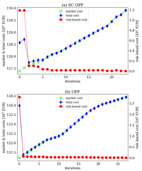
Figure 5.
The costs obtained in the risk optimization process for the SC OPF (a) and the OPF (b) scenarios: the market cost (green), the risk-based cost (red—plotted with respect to the right vertical axis) and the total cost—the sum of two former ones (blue) with minimal value after 2 iterations in (a) and 1 iteration in (b).
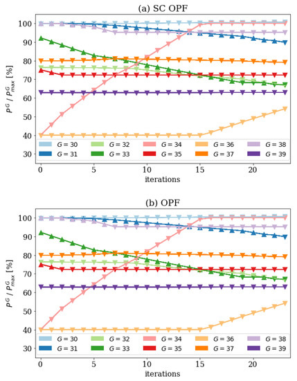
Figure 6.
The active power values () obtained in the risk optimization process for SC OPF (a) and OPF (b) scenarios and for every generator in each iteration (apart from Gen. 30 with constant generation level). The results include the identification of critical (CMs) and non-critical (NMs) machines, depicted by upward and downward triangles, respectively.
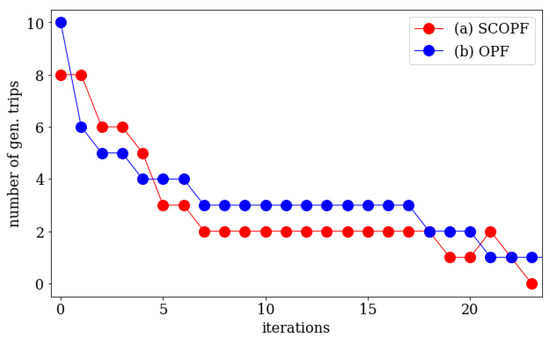
Figure 7.
The total number of all generator trips in each iteration obtained in the risk optimization process for SC OPF (red) and OPF (blue) scenarios.
In Figure 5a,b the evolution of three costs is depicted: the market one describing the cost resulting from the dispatch, the risk-based cost resulting from the dynamic risk assessment (expressing the expected value of the cost incurred by the TSO) and their sum - the total cost. The simulations were carried out until reaching the final stopping criterion given by (2), although the one defined by (3) was satisfied after 2 iterations in the SC OPF case and 1 in the OPF one. We can see that in the initial iteration the SC OPF dispatch is characterized by lower risk, which means that it provides not only N-1 static security but indirectly increases also dynamic stability. The reason for this behavior may be found in the fact that SC OPF, with its more restrictive constraints, provides a dispatch with greater values of power margins (see Table 1 or the initial iteration in Figure 6). In the case of OPF, the cheaper generators are loaded more heavily ( for 4 of them, with only 2 having this property in the SC OPF case) and as a consequence, they have lower transient stability margin. Furthermore, due to being more stable dynamically, the SC OPF converges quicker to the minimal risk, whereas the OPF, favoring cost-optimization, converges quicker to the minimum total cost.
The generation levels in each iteration are depicted in Figure 6, which also illustrates the identification of CMs and NMs (with upward and downward triangles, respectively). In Figure 7 the total number of generators tripped in each iteration is shown—in the OPF case this number and the risk (Figure 5b) decrease monotonically. This is not true for SC OPF (Figure 5a), due to the change of status from NM to CM by one of the units (Gen. 33 in 21st iteration). However, this is fixed in the following iteration and the whole process converges eventually. Such cases confirm the requirement to perform the power shifting in little steps. The importance of adjusting the factor, responsible for the power shifted in each iteration is also discussed in Section 3. Most importantly, the total cost after the final iteration with OPF, which is equal to the market cost of the dispatch characterized by no risk (), is lower than the initial market cost in SC OPF. The reason behind this effect is that the SC OPF provides a conservative solution allowing the system to withstand N-1 contingencies without corrective actions. On the other hand, dynamic simulations include some corrective actions, e.g., by the primary or secondary control and therefore they are able to relax the initial operating points. What is more, due to the fact that dynamic simulations incorporate also all static stability phenomena, we find that the dynamically extended OPF is more computationally and economically efficient than dynamically extended SC OPF.
Sensitivity Analysis
The sensitivity analysis of the dynamic risk optimization was applied in order to test the robustness of the proposed method against the amount of power shifted from CMs to NMs in one iteration. For that purpose, we performed the optimization process for SC OPF and OPF scenarios and for the following amounts of the shifted power . The results of the sensitivity analysis are shown in Figure 8 for SC OPF and OPF. The common factor for both scenarios is the inverse proportionality of and the number of iterations as well as the proportionality of and the total costs. Moreover, those figures also show that decreasing below a certain level does not necessarily result in lower total costs (both obtained at the minimum and at the final iteration), as they reach a plateau in the range below . Moreover, although the numbers of iterations taken to reach are lower in the SC OPF case, the numbers after which the minimum of the total cost (similar to (3)) were found, are lower in the OPF case. To sum up, the sensitivity analysis shows that at some point reducing does not alter the risk results. However, it significantly increases the numbers of iterations, making the computations longer and more expensive. Therefore, it could be found that there is a range of for which it is possible to find a compromise for both, the accuracy and computational costs.
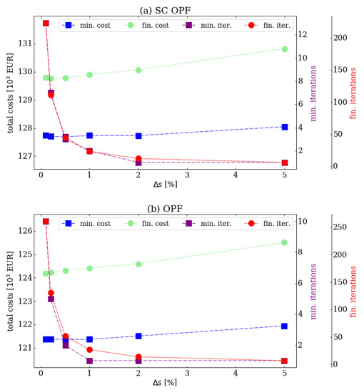
Figure 8.
Results of sensitivity analysis for SC OPF (a) and OPF (b) scenarios, and for two stopping criteria: min.—representing the minimal total cost as in (3) and fin.—representing the case with . The total costs for min. (blue) and fin. (green) are plotted with respect to the left vertical axis. The number of iterations (iter.) to reach the stopping criterion for min. (purple) and fin. (red) are plotted with respect to right separate vertical axes.
4. Conclusions
This paper proposed the iterative methodology of obtaining preventive remedial actions by extending the SC UC/ED with constraints based on the risk assessed for the power system. Two criteria were used, namely the risk minimization or the total cost minimization. In the latter case, only 2 or even 1 iteration (if SC conditions are relaxed) are required for the modified dynamic IEEE39 system. The method can be successfully used for off-line testing and, if contingency filtering screening techniques are applied, it has also the potential for day-ahead planning. However, the authors expect that with the growing availability and decreasing costs of distributed computing, going beyond day-ahead to intra-day processes will be possible in the future. In the presented test case, we limited the analysis to only one hourly dispatch, which simplified the SC UC/ED (UC/ED) problem to SC OPF (OPF) and made the results easier to interpret and present. However, the same way of reasoning works also for SC UC/ED, where the daily dispatch may be obtained. In such cases the constraints (for generators active power upper limits) are adjusted for each hour independently, still allowing the SC UC/ED tool to deliver a consistent solution for 24 h (satisfying its built-in inter-temporal constraints). The proposed methodology is general as significant flexibility is allowed with respect to the models of generators and protection relays along with the way to include their actions in calculating the costs. Moreover, it allows adapting the current operating points to variable weather conditions, which may be crucial for the accurate reliability analysis of the power system. Finally, the presented approach could be extended with the following:
- Utilizing contingency screening methods, like SIME used for the transient stability assessment, for the purpose of filtering the most critical contingencies.
- Extending the dynamic model of the power system with under- and overvoltage protection relays to include the costs of load shed due to voltage instabilities.
- Adjusting the value of power shifted from critical to non-critical machines from one iteration to another, e.g., basing on the risk reduction.
- Integrating the reactive power redispatch into the risk optimization process.
To conclude, the authors believe that the proposed risk-based redispatch optimization, although being heuristic, provides an interesting alternative planning procedure for TSOs in the future, yet allowing them to implement it without changing their current optimization engine. With the fact of being tunable on one hand and the increase of computational efficiency on another, the method may allow one to meet the requirements of future power systems, where the dynamic phenomena will play a significant role.
Author Contributions
Conceptualization, E.U.P., K.W. and W.J.; methodology, E.U.P., K.W.; software, W.J.; investigation, E.U.P., W.J.; data curation, R.K.; writing–original draft preparation, E.U.P., W.J.; writing–review and editing, E.U.P., K.W., W.J. and R.K.; visualization, W.J.; supervision, K.W., R.K.; formal analysis, K.W., E.U.P., R.K. and W.J.; funding acquisition, K.W. All authors have read and agreed to the published version of the manuscript.
Funding
This research was funded by the AXA Research Fund project “Development Of Methodology Assessing The Risk Of Remedial Actions In Transmission Systems And Optimizing Them”.
Conflicts of Interest
The authors declare no conflict of interest. The funders had no role in the design of the study; in the collection, analyses, or interpretation of data; in the writing of the manuscript, or in the decision to publish the results.
Appendix A. Example of Cost Calculation
For the purposes of this paper transmission lines failure rates published by the Polish TSO were used to obtain the probabilities of single transmission lines faults, simulated as 3-phase short-circuits. Whereas the costs were assigned to the following events:
- Tripping the synchronous generators by out-of-step protection relays included in the dynamic model,
- Shedding loads by under-frequency protection relays or disconnecting the load buses from the system.
Events of the first type were associated with a cost of starting up a synchronous generator from a standby mode, which was assumed to be the state of the generator after being tripped by the out-of-step relay. A constant value of was used for all generators in the IEEE39 system, which is a rough simplification made for the purpose of obtaining quantitative results (see Section 3). The cost of load shedding was associated with time and stage of the under-frequency relay action. Here is an example. Let us assume that during a contingency C (initiated by a fault at ), a generator was tripped at giving rise to the cost by . This was followed by frequency drop causing the action of load shedding relays in the first stage, which resulted in disconnecting 20% of the load, equal to at in one and at in another bus. If the consequences of C was accumulated over time (when the steady-state was achieved), the total cost is calculated using the value of lost load in the way shown in (A1):
Knowing the cost and probability allows us to obtain the contribution of every considered contingency to the risk given by (1).
References
- Wawrzyniak, K.; Padrón, E.U.; Gomulski, K.; Korab, R.; Jaworski, W. Methodology of risk assessment and decomposition in power grid applications. IET Gener. Transm. Distrib. 2018, 12, 3666–3672. [Google Scholar] [CrossRef]
- Gan, D.; Thomas, R.J.; Zimmerman, R.D. Stability-constrained optimal power flow. IEEE Trans. Power Syst. 2000, 15, 535–540. [Google Scholar] [CrossRef]
- Pizano-Martianez, A.; Fuerte-Esquivel, C.R.; Ruiz-Vega, D. Global Transient Stability-Constrained Optimal Power Flow Using an OMIB Reference Trajectory. IEEE Trans. Power Syst. 2010, 25, 392–403. [Google Scholar] [CrossRef]
- Alam, A.; Makram, E.B. Transient stability constrained optimal power flow. In Proceedings of the 2006 IEEE Power Engineering Society General Meeting, Montreal, QC, Canada, 18–22 June 2006. [Google Scholar]
- Pizano-Martínez, A.; Fuerte-Esquivel, C.R.; Zamora-Cárdenas, E.; Ruiz-Vega, D. Selective transient stability-constrained optimal power flow using a SIME and trajectory sensitivity unified analysis. Electr. Power Syst. Res. 2014, 109, 22–44. [Google Scholar] [CrossRef]
- Xu, Y.; Ma, J.; Dong, Z.Y.; Hill, D.J. Robust Transient Stability-Constrained Optimal Power Flow with Uncertain Dynamic Loads. IEEE Trans. Smart Grid 2017, 8, 1911–1921. [Google Scholar] [CrossRef]
- Ahmadi, H.; Ghasemi, H.; Haddadi, A.M.; Lesani, H. Two approaches to transient stability-constrained optimal power flow. Int. J. Electr. Power Energy Syst. 2013, 47, 181–192. [Google Scholar] [CrossRef]
- Fouad, A.A.; Jianzhong, T. Stability constrained optimal rescheduling of generation. IEEE Trans. Power Syst. 1993, 8, 105–112. [Google Scholar] [CrossRef]
- Kuo, D.H.; Bose, A. A generation rescheduling method to increase the dynamic security of power systems. IEEE Trans. Power Syst. 1995, 10, 68–76. [Google Scholar]
- Shubhanga, K.N.; Kulkarni, A.M. Stability-constrained generation rescheduling using energy margin sensitivities. IEEE Trans. Power Syst. 2004, 19, 1402–1413. [Google Scholar] [CrossRef]
- Kim, K.H.; Rhee, S.B.; Hwang, K.J.; Song, K.B.; Lee, K.Y. Generation rescheduling based on energy margin sensitivity for transient stability enhancement. J. Electr. Eng. Technol. 2016, 11, 20–28. [Google Scholar] [CrossRef][Green Version]
- Hoballah, A.; Erlich, I. Generation coordination for transient stability enhancement using particle swarm optimization. In Proceedings of the 12th International Middle-East Power System Conference (MEPCON 2008), Aswan, Egypt, 12–15 March 2008. [Google Scholar]
- Nguyen, T.B.; Pai, M.A. Dynamic security-constrained rescheduling of power systems using trajectory sensitivities. IEEE Trans. Power Syst. 2003, 18, 848–854. [Google Scholar] [CrossRef]
- Li, Y.H.; Yuan, W.P.; Chan, K.W.; Liu, M.B. Coordinated preventive control of transient stability with multi-contingency in power systems using trajectory sensitivities. Electr. Power Syst. Res. 2011, 33, 147–153. [Google Scholar] [CrossRef]
- Fang, D.Z.; Sun, W.; Xue, Z.Y. Optimal generation rescheduling with sensitivity-based transient stability constraints. IET Gener. Transm. Distrib. 2010, 4, 1044–1051. [Google Scholar] [CrossRef]
- Kucuktezcan, C.F.; Genc, V.M.I. A new dynamic security enhancement method via genetic algorithms integrated with neural network based tools. Electr. Power Syst. Res. 2012, 83, 1–8. [Google Scholar] [CrossRef]
- Kundur, P.; Balu, N.J.; Lauby, M.G. Power System Stability and Control, 7th ed.; McGraw-Hill: New York, NY, USA, 2016. [Google Scholar]
- Wang, J.; Xiong, X.; Zhou, N. Time-varying failure rate simulation model of transmission lines and its application in power system risk assessment considering seasonal alternating meteorological disasters. IET Gener. Transm. Distrib. 2016, 10, 1582–1588. [Google Scholar] [CrossRef]
- He, D.; Zhang, Y.; Guo, C. Failure probability model of transmission and transformation equipment for risk assessment. In Proceedings of the Power and Energy Society General Meeting (PESGM 2016), Boston, MA, USA, 17–21 July 2016. [Google Scholar]
- Polskie Sieci Elektroenergetyczne (PSE). Available online: https://www.pse.pl/web/pse-eng (accessed on 6 February 2020).
© 2020 by the authors. Licensee MDPI, Basel, Switzerland. This article is an open access article distributed under the terms and conditions of the Creative Commons Attribution (CC BY) license (http://creativecommons.org/licenses/by/4.0/).