Accurate Location of Faults in Transmission Lines by Compensating for the Electrical Distance


1
School of Electrical and Power Engineering, China University of Mining and Technology, Xuzhou 221116, China
2
Jiangsu Province Laboratory of Mining Electric and Automation, Xuzhou 221116, China
*
Author to whom correspondence should be addressed.
Energies 2020, 13(3), 767; https://doi.org/10.3390/en13030767
Submission received: 30 December 2019
/
Revised: 24 January 2020
/
Accepted: 5 February 2020
/
Published: 10 February 2020
Abstract
:Accurately locating faults is quite important, especially when the geographical environment is complicated. If the exact location of the fault is not given, wrong route would be chosen, which will greatly slow down repair. This paper proposes an improved traveling wave method by compensating the electrical distance of transmission lines. The catenary model is constructed that considers parameters of the tower and the actual temperature. The actual line length is also derived by the catenary model. A 500 kV transmission line model is established by PSCAD/EMTDC. Various fault simulations are conducted and the results demonstrate that the presented method effectively reduces the error ratio of faulty segment positioning and locates faults with high accuracy.
1. Introduction
With the rapid development of the power industry and the continuous expansion of power systems, the voltage level and transmission capacity of transmission lines are gradually growing, and the number of high-voltage transmission lines is also increasing [1,2,3]. However, high-voltage transmission lines often travel across complex terrain and are exposed to the wild all year round. They are prone to faults due to bad weather conditions and other factors, resulting in huge losses to industrial production and the economy [4,5]. Therefore, it is of great significance to quickly and accurately locate faults in transmission lines [6,7]. Accurate fault location can improve the efficiency of troubleshooting, reduce outage times, and increase system stability [8].
The main fault location methods are the impedance and traveling wave methods [9,10]. Most methods directly take the sum of the horizontal distance between towers as the total length of the transmission line [11,12,13]. However, the actual length will be affected by sag, temperature, and the level of the load current [14,15]. According to the principles of fault location methods [16,17,18], the length of the transmission line is an important factor that affects the accuracy of fault location. Taking a 500 kV transmission line as an example, according to the Code for the design of 110 kV–750 kV overhead transmission lines [19], the total height of the transmission line tower is generally 30-50 m, and the minimum distance from the wire to the ground is at most 14 meters. It is assumed that the height of the tower is 40 m, and the length of the transmission line is 40 km. According to the simplified computational model shown in Figure 1, the actual length of the line is 40.447 km. Therefore, the correction of the length of the transmission line is of importance to improve the positioning accuracy.
In addition, accurate positioning results can improve the efficiency of excluding the fault. As most faults happen when the weather is terrible or the geographic environment is complicated, incorrect results will cause trouble to the maintainer. Figure 2 shows two towers, B and C, that are built over a river. If the fault happens at the end of line AB, when the wind span is used to locate the fault, it is possible that the fault will be positioned at F’ between B and C. Not only are F and F’ located at the two sides of tower B, but also on both sides of the river. An incorrect section location will mislead the maintainer about the path that should be chosen and reduce the efficiency with which the fault is tripped out.
Aiming at the problem mentioned above, we first establish a catenary model of the transmission line, and propose a method for calculating sag. Secondly, we consider the influence of temperature on the length of the transmission line in order to compensate for the electrical distance of the transmission line. Finally, a 500 kV transmission line is built in PSCAD/EMTDC to verify the practicability and accuracy of the proposed method.
2. Compensation for the Electrical Distance of Transmission Lines
In practical engineering application, geometric models of transmission line conductors are complicated due to such factors as the distribution of load current and the conductor’s rigidity. To simplify the construction of geometric model, we make the following two assumptions. First, the transmission line is assumed to be a flexible chain without any rigidity, which indicates that the conductor’s rigidity barely affects the space curve’s shape. Second, the load current is assumed to be uniformly distributed along the conductor [20,21,22]. To ensure the accuracy of the model’s construction, the geometric model of a transmission line conductor was established based on a catenary model [23].
Taking the lowest point of the conductor as the origin, a two-dimensional cartesian coordinate system was constructed as shown in Figure 3. In Figure 3, A and B represent the two suspension points of the conductor terminals. Force analysis of an arbitrary point P in the conductor was performed and is shown in Figure 4. The dead-weight of the conductor segment OP is denoted G, the horizontal stress of OP is denoted σ, and oblique stress is shown as F2.
According to the equilibrium equation, we have
where dx is the length of OP, α is the angle between F2 and the horizontal line, and ω represents a specific gravity load. According to (1), the following curve function expression can be obtained:
At the origin, y = 0, x = 0, and C = −σ/ω. Thus,
Equation (3) is the mathematical expression of the catenary model of the transmission line. In Figure 3, it is assumed that the coordinates of A and B are (−a, l1) and (L − a, l1+H), respectively. l1 is the vertical distance between A and the origin. H represents the difference in altitude between suspension points A and B. L denotes the line span. By taking the derivative of (3), we have
According to the basic principle for calculating arc length, the arc length L′ is
In addition, it can be observed that
Combining (5) and (6), we have
Based on the above analysis, it is clear that the higher the altitude difference between A and B, the larger the line span, and thus the longer the arc length of the line.
The maximum sag is one of the most important parameters for the safe operation of transmission lines. According to the catenary model, the function of the curve between A and B can be expressed by
The sag height of any point in the conductor is
To determine the maximum sag, the derivative of f(x) is calculated by
Thus, the maximum sag fh and the corresponding abscissa xh are
Under actual field conditions, the external environment and load current affect the temperature of the transmission lines in operation. When the current flows through the line conductors, the current-generated heat results in a significant increase in the temperature of the line. Although a portion of the heat will dissipate into the air, the temperature of the conductors will remain in a stable state. The increase in temperature leads to the expansion and contraction of the conductor. The expanded (or contracted) length L1 of the line conductor can be expressed as
where β is the expansion and contraction coefficient, t0 is the standard temperature, and t represents the current temperature of the conductor. Thus, the total length of the conductor, considering the effect of temperature, can be calculated by
From (13), the actual length of the transmission line is affected mainly by horizontal stress, gravity load, and temperature. These are the parameters of the transmission line itself and cannot be ignored.
The annual mean temperature in China is about 10 °C. The highest temperature in most parts of China is less than 40 °C. According to the technical specification for the design of 500 kV overhead transmission lines, the highest temperature of the transmission lines should be less than 70 °C and that in the eastern area should not exceed 80 °C. Taking an LGJ-300/40 mm2 steel-cored aluminum strand as an example. The load-to-weight ratio is 35.06 × 10⁻³ MPa/m, and the horizontal stress is 53.955 MPa. Based on the length of the conductor at 15 °C, the variations in the actual length with different temperatures and line spans are shown in Figure 5. From Figure 5, it can be seen that the variation in the line length grows as the temperature increases. At the same temperature, the larger the line span, the more significant the variation in length, which indicates that the length of the line is more susceptible to temperature in high-voltage and long-distance systems.
3. Simulation and Results
3.1. The influence of different fault locations
A 500 kV transmission line with 80 towers is built in PSCAD. The length of each span is 442.25 m, and the length of the whole line is 35.380 km. If the actual distance model is used, the actual length of each span is 443.6960 m and the length of the whole line is 35.459 km. In order to explore the effects of different fault locations on this method, the faults is set at the front end, in the middle, and at the tail of the line respectively.
In the electrical distance model, it is assumed that single-phase faults happen at 4.5224 km, 17.790 km, and 31.0575 km from the front end of the line. The model of the transmission line is shown in Figure 6. The voltage traveling wave signals were collected at Terminal A and Terminal B of the line. The sampling frequency was 10 MHz. The fault inception time was 0.08 s, and the simulation time was 0.09 s.
Transmission line models with electrical distance were built in PSCAD. Figure 7 shows the line-mode traveling wave fronts arriving at both ends of the line in terms of electrical distance. t1, t2 are the times at which the line-mode wave head arrives at both ends of the line. According to the principle of two-terminal fault location, the location results are shown in Table 1.
From the data presented above, it is clear that when a fault happens at the tail of the line, the influence of length on accuracy is more obvious. Therefore, the method proposed in this paper is more effective in correcting faults that happen near the end of the line.
3.2. The Influence of Different Temperatures
Taking 15 °C as the basis, transmission line models under −10 °C and 35 °C at the electrical distance were built. The simulation conditions and process were the same as those described in Section 3.1. It is assumed that a fault happens between tower 070 and tower 071 at a distance of 200 m from tower 070. The results are shown in Table 2.
According to Table 2, when the temperature varies, the length of the transmission line will also change, and this will have a certain impact on the positioning accuracy. The effect is more obvious at lower temperatures.
3.3. Engineering Practice
Taking a 500 kV transmission line in China as an example. The transmission line starts at the YL transformer substation and ends at the AT transformer substation. The total length of the line is 58.817 km. The distribution of the line is shown in Figure 8. The overhead conductor is an LGJ-630/45 mm2. Its specific gravity load is 57.0337 × 10⁻³ MPa/m, and the horizontal stress is 86.445 MPa. The expression for the overhead line is
When the temperature effect is not taken into account, the actual length of the line is
The model is shown in Figure 9. It is assumed that a single-phase earth fault occurs at 28.224 km from the head end of the line, that is, according to the electrical length, the fault occurs between tower 047 and tower 048 at a distance of 580 m from tower 047. The voltage traveling wave signals were collected at Terminal A and Terminal B of the line. The sampling frequency is 10 MHz, the fault inception time is 0.08 s, and the simulation time is 0.09 s.
According to the actual length of the line between the two towers, the fault happens between tower 047 and tower 048 at a distance of 406.222 m from tower 039. The actual fault location is shown in Figure 10.
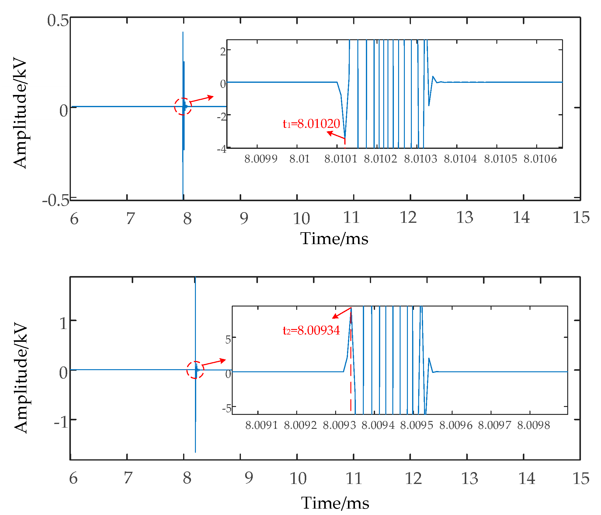
A transmission line model with electrical distance was built in PSCAD. Wavelet analysis was used to capture the time when the line-mode traveling wave heads arrived at both terminals of the line. Figure 11 shows the line-mode traveling wave fronts arriving at both ends of the line when the distance between the two towers was the electrical distance. t1, t2 are the times at which the line-mode wave heads arrive at both ends of the line. According to the principle of two-terminal fault location, the location results are shown in Table 3.
According to Table 3, it can be seen that the fault actually occurs between tower 047 and tower 048. However, due to the inaccurate calculation of the line’s length, the result incorrectly positions the fault between tower 048 and tower 049. In particular, because towers 048 and 049 are constructed over a river, the incorrect positioning results will cause maintenance to not be able to remove the fault quickly. Therefore, the method proposed in this paper is able to effectively reduce the error rate of segment location.
4. Conclusions
In this paper, the effects of sag and temperature were considered in order to correct the length of the line used to locate faults in transmission lines. A catenary model was used to correct the length of the line. Simulation results show that the correction that the proposed method provides is much more effective for faults that happen at the tail of the line than for faults that happen at the front end of the line. Second, when the temperature is extremely high or low, the effect of this method is more obvious, which makes it much more efficient for areas with large changes in temperature or extreme temperatures. Finally, this method can increase the accuracy of a faulty line segment’s identification and reduce the error rate of fault location. For faults that occur near a tower, it can effectively reduce the probability of a misjudgment in the line segment’s identification.
Author Contributions
Conceptualization: X.X.; Methodology: M.C., T.H., and G.W.; Validation: X.X., M.C., and N.P.; Formal Analysis: M.C., T.H., and G.W.; Writing—Original Draft Preparation: X.X. and M.C.; Writing—Review & Editing: X.X., M.C., G.W., and R.L.; Visualization: T.H. All authors have read and agreed to the published version of the manuscript.
Funding
This research was funded by The Fundamental Research Funds for the Central Universities (Grant No. 2019GF06).
Conflicts of Interest
The authors declare no conflicts of interest.
References
- Peng, N.; Cheng, M.; Liang, R.; Firuz, Z. Asynchronous fault location scheme for half-wavelength transmission lines based on propagation characteristics of voltage travelling waves. IET Gener. Transm. Dis. 2019, 13, 502–510. [Google Scholar]
- Ahmet, M.V. Contribution of high voltage direct current transmission systems to inter-area oscillation damping: A review. Renew. Sustain. Energy Rev. 2016, 57, 892–915. [Google Scholar]
- Peng, N.; Zhou, L.; Liang, R.; Xu, H. Fault location of transmission lines connecting with short branches based on polarity and arrival time of asynchronously recorded traveling wave. Electr. Power Syst. Res. 2019, 169, 184–194. [Google Scholar] [CrossRef]
- Naidu, O.D.; Pardahan, A.K. A traveling wave-based fault location method using unsynchronized current measurements. IEEE Trans. Power Deliv. 2019, 34, 505–513. [Google Scholar] [CrossRef]
- Aleena, S.; Anamika, Y. A novel single-ended fault location scheme for parallel transmission lines using k-nearest neighbor algorithm. Comput. Electr. Eng. 2018, 69, 41–53. [Google Scholar]
- Ahmed, S.; Ahmed, E.; Hany, E. New fault location scheme for three-terminal untransposed parallel transmission lines. Electr. Power Syst. Res. 2018, 154, 266–275. [Google Scholar]
- Ahmad, S.D.; Ali, M.R. A wide-area scheme for power system fault location incorporating bad data detection. IEEE Trans. Power Deliv. 2015, 30, 800–808. [Google Scholar]
- Abu, S.; Saif, M. A new on-line technique to identify fault location within long transmission lines. Eng. Fail. Anal. 2019, 105, 52–64. [Google Scholar]
- Fei, C.; Qi, G.; Li, C. Fault location on high voltage transmission line by applying support vector regression with fault signal amplitudes. Electr. Power Syst. Res. 2018, 160, 173–179. [Google Scholar] [CrossRef]
- Jiao, B. A New Method to Improve Fault Location Accuracy in Transmission Line Based on Fuzzy Multi-Sensor Data Fusion. IEEE Trans. Smart Grid 2019, 10, 4211–4220. [Google Scholar] [CrossRef]
- Lopes, F.V.; Silva, K.M.; Costa, F.B.; Neves, W.L.A.; Fernandes, D., Jr. Real-time traveling-wave-based fault location using two-terminal unsynchronized data. IEEE Trans. Power Deliv. 2015, 30, 1067–1076. [Google Scholar] [CrossRef]
- Rahman, D.; Mohammad, D.; Hamid, R.S.; Maryamsadat, T. Impedance-based fault location method for four-wire power distribution networks. IEEE Access. 2018, 6, 1342–1349. [Google Scholar]
- Benato, R.; Sessa, S. An online traveling wave fault location method for unearthed-operated high-voltage overhead line grids. IEEE Trans. Power Deliv. 2018, 33, 2776–2785. [Google Scholar] [CrossRef]
- Chen, Y.; Tan, J.; Liu, W.; Chen, S.; Zhu, F. Analysis on main factors impacting length of transmission line. Power Syst. Technol. 2007, 31, 41–44. [Google Scholar]
- Peng, X.; Mao, X.; Li, X.; Zhang, F. Errors analysis of overhead transmission line fault location based on distributed travelling-wave. High Volt. Eng. 2013, 39, 2706–2713. [Google Scholar]
- Chen, Y.; Liu, D. Wide-area traveling wave fault location system based on IEC61850. IEEE Trans. Smart Grid 2013, 4, 1207–1255. [Google Scholar] [CrossRef]
- Lopes, F. Setting-free traveling-wave-based earth fault location using unsynchronized two-terminal data. IEEE Trans. Power Deliv. 2016, 31, 2296–2298. [Google Scholar] [CrossRef]
- Zhang, G.; Shu, H.; Liao, Y. Automated double-ended traveling wave record correlation for transmission line disturbance analysis. Electr. Power Syst. Res. 2016, 136, 242–250. [Google Scholar] [CrossRef]
- China Electricity Council. GB50545-2010. Code for Design of 110 kV–750 kV Overhead Transmission Line; China Planning Press: Beijing, China, 2010. [Google Scholar]
- Polevoy, A. Impact of data errors on sag calculation accuracy for overhead transmission line. IEEE Trans. Power Deliv. 2014, 29, 2040–2045. [Google Scholar] [CrossRef]
- Dong, X. Analytic method to calculate and characterize the sag and tension of overhead lines. IEEE Trans. Power Deliv. 2016, 31, 2064–2071. [Google Scholar] [CrossRef]
- Jiang, J.; Jia, Z.; Wang, X.; Wang, S.; Yang, C. Analysis of conductor sag change after bare overhead conductor is covered with insulation material. In Proceedings of the 2nd International Conference on Electrical Materials and Power Equipment, Guangzhou, China, 7–10 April 2019. [Google Scholar]
- Liu, Y.; Sheng, G.; Sun, S.; Gao, X. A Method for Fault Location Compensation Considering Operating States of Transmission Lines. Autom. Electr. Power Syst. 2012, 36, 92–96. [Google Scholar]
Figure 1.
Simplified computational model of a transmission line.

Figure 2.
Schematic diagram of a tower across a river.
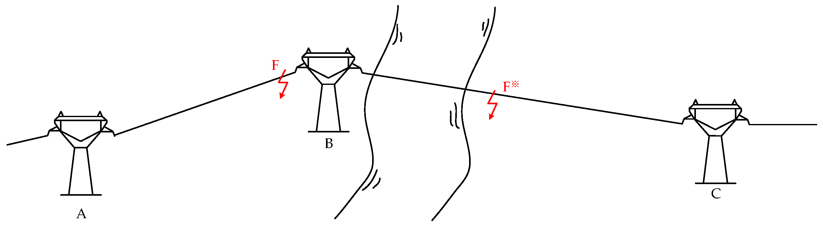
Figure 3.
Model of an unequal-altitude catenary.

Figure 4.
Force diagram of the OP conductor segment.

Figure 5.
Length variations with different temperatures and conductor line lengths.

Figure 6.
The model of the transmission line when faults happen (a) in different parts of the line, (b) in the middle of the line, and (c) at the tail of the line.
Figure 6.
The model of the transmission line when faults happen (a) in different parts of the line, (b) in the middle of the line, and (c) at the tail of the line.


Figure 7.
A line-mode traveling wave waveform in the electrical distance model when faults happen (a) in different parts of the line, (b) in the middle of the line, and (c) at the tail of the line.
Figure 7.
A line-mode traveling wave waveform in the electrical distance model when faults happen (a) in different parts of the line, (b) in the middle of the line, and (c) at the tail of the line.


Figure 8.
The distribution of the 500 kV transmission line.

Figure 9.
Schematic diagram of the 500 kV transmission line in terms of electrical distance.
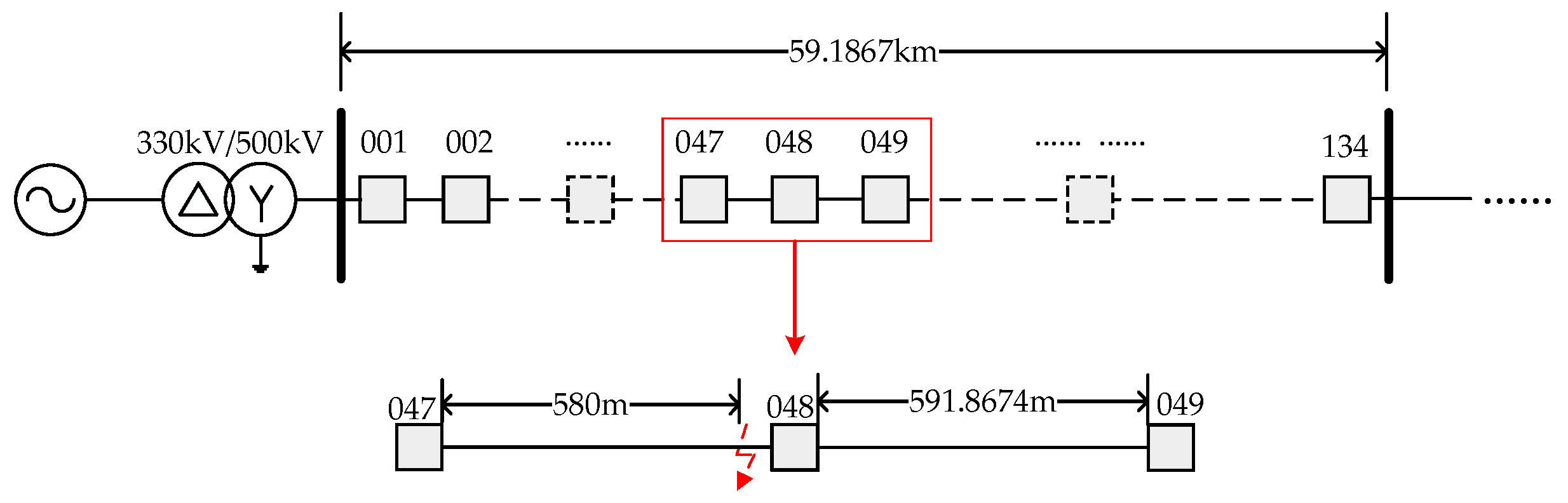
Figure 10.
Schematic diagram of the 500 kV transmission line in terms of actual distance.

Figure 11.
The line-mode traveling wave waveform in the actual distance model.

Table 1.
Comparison of fault location results from the electrical and actual distance models.
| Fault Location | Electrical Distance | Actual Distance |
|---|---|---|
| at the front of the line | between 010 and 011 215.6 m from 010 | between 010 and 011 201.14 m from 010 |
| in the middle of the line | between 040 and 041 277.25 m from 039 | between 040 and 041 220.856 m from 039 |
| at the tail of the line | between 070 and 071 201.9 m from 070 | between 070 and 071 100.68 m from 070 |
Table 2.
Comparison of fault location results from the electrical and actual distance models.
| Temperature | Electrical Distance | Actual Distance | ||||
|---|---|---|---|---|---|---|
| Line Length | Presupposed Fault Location | Fault Location | Line Length | Presupposed Fault Location | Fault Location | |
| −10 °C | 35.363 | between 070 and 071 199.9050 m from 070 | between 070 and 071 163.903 m from 070 | 35.4888 | between 070 and 071 90.019 m from 070 | between 070 and 071 54.017 m from 070 |
| 15 °C | 35.38 | between 070 and 071 200 m from 070 | between 070 and 071 201.9 m from 070 | 35.49 | between 070 and 071 98.78 m from 070 | between 070 and 071 100.68 m from 070 |
| 35 °C | 35.393 | between 070 and 071 200.067 m from 070 | between 070 and 071 187.33 m from 070 | 35.519 | between 070 and 071 92.196 m from 070 | between 070 and 071 70.129 m from 070 |
Table 3.
Comparison of fault location results from the electrical and actual distance models.
| The Way of Calculating The Distance Line | Electrical Distance | Actual Distance |
|---|---|---|
| Fault location (km) | between 047 and 048, 580 m from 047 | between 047 and 048, 406.22m from 047 |
| Location results | between 048 and 049, 14.14 m from 048 | between 047 and 048, 428.5322 m from 047 |
© 2020 by the authors. Licensee MDPI, Basel, Switzerland. This article is an open access article distributed under the terms and conditions of the Creative Commons Attribution (CC BY) license (http://creativecommons.org/licenses/by/4.0/).
Share and Cite
MDPI and ACS Style
Xue, X.; Cheng, M.; Hou, T.; Wang, G.; Peng, N.; Liang, R. Accurate Location of Faults in Transmission Lines by Compensating for the Electrical Distance. Energies 2020, 13, 767. https://doi.org/10.3390/en13030767
AMA Style
Xue X, Cheng M, Hou T, Wang G, Peng N, Liang R. Accurate Location of Faults in Transmission Lines by Compensating for the Electrical Distance. Energies. 2020; 13(3):767. https://doi.org/10.3390/en13030767
Chicago/Turabian StyleXue, Xue, Menghan Cheng, Tianyu Hou, Guanhua Wang, Nan Peng, and Rui Liang. 2020. "Accurate Location of Faults in Transmission Lines by Compensating for the Electrical Distance" Energies 13, no. 3: 767. https://doi.org/10.3390/en13030767
Note that from the first issue of 2016, this journal uses article numbers instead of page numbers. See further details here.