Hydrate—A Mysterious Phase or Just Misunderstood?

1
State Key Laboratory of Oil and Gas Reservoir Geology and Exploitation, Southwest Petroleum University, Xindu Road No.8, Chengdu 610500, China
2
Environmental Engineering Department, University of California Irvine, Irvine, CA 92697, USA
*
Author to whom correspondence should be addressed.
Energies 2020, 13(4), 880; https://doi.org/10.3390/en13040880
Submission received: 6 December 2019
/
Revised: 12 February 2020
/
Accepted: 13 February 2020
/
Published: 17 February 2020
(This article belongs to the Special Issue Integration of Theoretical, Laboratory, and Field Studies for Efficient Gas Hydrate Assessment and Acquisition)
Abstract
:Hydrates that form during transport of hydrocarbons containing free water, or water dissolved in hydrocarbons, are generally not in thermodynamic equilibrium and depend on the concentration of all components in all phases. Temperature and pressure are normally the only variables used in hydrate analysis, even though hydrates will dissolve by contact with pure water and water which is under saturated with hydrate formers. Mineral surfaces (for example rust) play dual roles as hydrate inhibitors and hydrate nucleation sites. What appears to be mysterious, and often random, is actually the effects of hydrate non-equilibrium and competing hydrate formation and dissociation phase transitions. There is a need to move forward towards a more complete non-equilibrium way to approach hydrates in industrial settings. Similar challenges are related to natural gas hydrates in sediments. Hydrates dissociates worldwide due to seawater that leaks into hydrate filled sediments. Many of the global resources of methane hydrate reside in a stationary situation of hydrate dissociation from incoming water and formation of new hydrate from incoming hydrate formers from below. Understanding the dynamic situation of a real hydrate reservoir is critical for understanding the distribution characteristics of hydrates in the sediments. This knowledge is also critical for designing efficient hydrate production strategies. In order to facilitate the needed analysis we propose the use of residual thermodynamics for all phases, including all hydrate phases, so as to be able to analyze real stability limits and needed heat supply for hydrate production.
1. Introduction
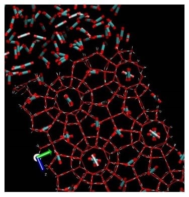
The formation of hydrocarbon hydrates has been a problem for the oil and gas industry for many decades. Macroscopically these hydrates looks like ice or snow. Industrially the most important structures are structure I and structure II. The smallest symmetric unit in structure I is a cubic cell containing 46 water molecules, which creates two small cavities and six large cavities formed by hydrogen bounded water. In structure I the smallest cavities consists of 20 water molecules in the cavity walls and for the large cavity there are 24 water molecules in the cavity walls (see Figure 1 for an illustration). The cavities are stabilized mainly by the volume of the molecules (repulsion) entering the cavities and weak van der Waal type attractions between the molecules in the cavity and the water molecules in the cavity walls. Molecules of limited polarity can also enter these cavities. The dipole moment of H2S leads to a positive net charge in direction outwards from center of mass when the molecules rotate in the cavity. Samplings from molecular dynamics simulations [1] show that the result of the water molecules in the cavity walls is a net negative charged Coulombic field pointing inwards in the cavity. The extra attractive coulombic energy between water and H2S [2], as compared to neutral molecules like for instance methane, is the reason why H2S is an exceptionally good hydrate former. CO2, on the other hand, has a significant quadrupole moment which results in a negative coulombic field in the direction outward from center of mass. The result is a Coulombic repulsion that destabilizes the large cavity in structure I hydrate by roughly 1 kJ/mole hydrate [2]. The large size of the CO2, relative to the size of the large cavity, destabilizes the structure I hydrate further with approximately 1 kJ/mole hydrate [1]. These destabilization effects are still limited compared to the effects of fairly large attractive van der Waal attractions between water and the three atoms in CO2. These aspects are one of the reasons that CO2 is a substantially better hydrate former than for instance CH4. This will be quantified in more details later. An aspect that is rarely discussed is the stabilizing effects due to attractions between molecules inside neighboring cavities. An old study this was published by Kvamme and Lund [3] using a Monte Carlo method. These attractions between molecules in neighboring cavities are significant and often corrected for by empirical correction factors. Some of these can be found in the book by Sloan and Koh [4] and will not be discussed in more detail here.
Structure II hydrate contains 16 small cavities and eight large cavities with a total of 136 water molecules in a unit cell with side lengths 17 Å. The small cavity is similar to the small cavity in structure I but the large cavity in structure II is larger and contains 28 water molecules in the cavity walls. The large cavity has space for molecules like for instance propane and iso-butane. In order to limit the scope of this paper we will mostly focus on structure I hydrates for a variety of reasons. Mostly because the discussion in this paper focus very much on hydrate non-equilibrium but also because 99% of natural gas hydrate resources in the world are from biogenic degradation of organic material and the resulting hydrocarbons are almost pure methane. CO2 also makes hydrate structure I and the possible win-win situation of simultaneous CO2 storage as hydrate and release of CH4 from in situ hydrates is another motivation for this paper.
Van der Waal and Platteeuw [7] used a semi-grand canonical ensemble to derive a Langmuir type adsorption theory in which water molecules are fixed and rigid while molecules that enter cavities (guest molecules) are open to exchange with surrounding phases. The final result of the derivation is expressed in terms of chemical potential for water in hydrate:
where is the chemical potential for water in an empty clathrate for the given structure in consideration. Historically thus value has not been calculated by theoretical methods but rather fitted to experimental data in the form of chemical potential of pure liquid water minus empty clathrate water chemical potential. See Sloan and Koh [4] for some examples of values. K is an idex for cavity types and j is an index for guest molecules in the various cavities. Number of cavities is ν, with bubscripts k for large and small cavities respectively. For structure I, which is the main focus here, νøarge = 3/24 and νsmall = 1/24. For structure II the corresponding numbers are νlarge = 1/17 and νsmall = 2/17. Since this is a thermodynamic paper it is not necessary to list many details on the differences between these two structures other than the differences in chemical potentials for water in the two structures as given in Figure 2 below, and the distribution of cavities. Furthermore we can even limit ourselves to structure I hydrates since our main focus is to discuss the non-equilibrium nature of hydrates in sediments, and in industrial situations. Generally we should expect this to be trivial since it is well known that only one of temperature or pressure can be controlled in measurements of hydrate equilibrium. With both themperature and pressure defined locally in a sediment the system is overdetermined by one thermodynamic variable when hydrate former phase, liquid water and hydrate is present, but due to gas/water/hydrate/mineral interactions the system is even more mathematically overdetermined. In an overdetermined system the general equlibrium equations does not apply and free energy minimum under constraints of mass and energy determines local distribution of phases and associated compositions. The motivation of this paper is to illustrate that hydrates cannot reach equilibrium, and that hydrate can form and dissociate through a variaty of differeent phase transitions.
The canonical partititon fuctions for the cavities, hij that will be a result of the grand canonical derivation will generally be an exponential function of the chemical potential time Boltzmann integrals over interactions between guests and water (generally also with surrounding guest molecules [3]). In the classical formulation of van der Waal and Platteeuw [7] the result for a rigid lattice is:
The Langmuir constant for a molecule i in cavity k and given below as Equation (3). In the simplest case of a monoatomic spherical guest molecules the Langmuir constant is a simple integral over the Boltzmann factors of interaction energies between the guest molecule and surrounding waters:
For non-linear multi-atomic representations of guest molecules the integration will involve rorational degrees of freedom. is the interaction energy between water and guest molecules. x, y and z are volumetric coordinates. β is the inverse of temperature time Boltzman’s constant. is Boltzmann’s constant.
The most common guest/water interaction model in present versions hydrate equilibrium codes based of the reference method is based on a spherically smeared out version of the Kihara potential for interactions between a water and a guest. The Kihara potential can be expressed as:
where i and j are molecular indexes while is the closest distance between the two molecules. is a molecular diameter and is a well-depth. For aij equal to zero Equation (4) reduces to the Lennad-Jones 12-6 potential. A summation of approximate pariwise interactions in Equation (3) is possible and integration can be conducted efficiently using a Monte Carlo approach [2,3]. It is, however, more common to use an integrated smeared interaction version in which the average water/guest interaction are smeared out over the surface of a spherically smoothed cavity radius R. z is used as the number of waters represented in this spherical shell in Equation (4) below. Z is therefore 20 for small cavity and 24 for large cavity. The details of this integration to reach at the spherically smoothed potential is far too extensive to include here. See reference [4] for more details and further references as well as examples of values for Equation (4). The final results is for each specific cavity k is:
The sperically symmetric integration version of Equation (3) can then be expressed as:
Kvamme and Tanaka [1] also utilized a semi-grand canonical ensemble and used molecular dynamics simulations to derive the same equation as Equation (1) but the meaning of chemical potential is now physically average sampled chemical potential of water in empty clathrate based on a harmonic oscillator approach. These chemical potentials are therefore denoted as reference chemical potentials. Values for water chemical potential in empty clathrates of structures I and II are plotted in Figure 2 below.
Chemical potentials for water in empty clathrates of structures I and II, as well as in ice and liquid water, is reported by Kvamme and Tanaka [1] but a simpler and even more useful form of fit is the following equation:
Parameters for Equation (8) are given Table 1 below
A rigid water lattice model similar to Equation (3) is also available in the formalism of Kvamme and Tanaka [1], and will be more accurate than the and harmonic oscillator approach for small guest guest molecules relative to cavity size. For CH4 the harmonic oscillator model, and a rigid water lattice integral, gives almost the same result. The harmonic oscillator approach is superior for larger guest molecules relative to cavity size. The harmonic oscillator approach can be expressed as:
where β is the inverse of the universal gas constant times temperature. At equilibrium, the chemical potential of the guest molecules i in hydrate cavity k are equal to the chemical potential of molecules i in the co-existing phase it comes from. For non-equilibrium, the chemical potential is adjusted for distance from equilibrium through a Taylor expansion as discussed later. The free energies of inclusion (latter term in the exponent) are reported elsewhere [8,9,10,11,12,13]. At thermodynamic equilibrium between a free hydrate former phase, μki is the chemical potential of the guest molecule in the hydrate former phase (gas, liquid, or fluid) at the hydrate equilibrium temperature and pressure.
The composition of the hydrate is also trivially given by the derivation from the semi Grand Canonical ensemble and given by:
is the filling fraction of component i in cavity type k. Also:
where ν is the fraction of cavity per water for the actual cavity type, as indicated by subscripts. The corresponding mole-fraction water is then given by:
and the associated hydrate free energy is then:
Outside of equilibrium the corresponding result for a Taylor expansion is given by:
The paper is organized as follows: Motivation and objectives are given in the next section. Some reflection on hydrate non-equilibrium during pipeline transport of hydrate forming fluids with water is discussed in Section 3. Non-equilibrium aspects of hydrates in sediments are discussed in Section 4. A discussion is given in Section 5 and our conclusions complete the paper.
2. Motivation and Objectives
Analysis of hydrate problems during pipeline transport of hydrocarbons or other hydrate forming fluids like for instance CO2 is typically oversimplified. Frequently the analysis is based on independent tthermodynamic variables rather than the associated thermodynamic functions. The combined first and second laws of thermodynamics states that Gibbs Free energy always will strive towards local minimum as function of temperatures, pressures and masses in the system, under constraints of mass and heat transport. In non-equilibrium systems it is the total extensive Gibbs free energy minimum that determines phase distributions and compositions. Practically this implies that chemical potentials for the various components in different phases are not the same. Hydrate can never reach full thermodynamic equilibrium in pipeline transport, or in sediments in nature, because there are too many active phases that interacts with the hydrate phases.
The first objective of this work is to demonstrate a thermodynamic toolbox based on residual thermodynamics for all phases, including hydrate phases. We also show how water in ice, liquid water and empty hydrates can be simply correlated so that any group can make use of this concept instead of using empirically fitted chemical potential differences based on calculation methods from around 1970. This opens up for calculations of many hydrate phase transitions that leads to hydrate formation, and other routes that leads to hydrate dissociation. Residual thermodynamic calculations of hydrates provide direct comparison between hydrates formed from different phases. Hydrates formed from methane gas and liquid water will have a different composition than hydrate formed from methane dissolved in water. These hydrates will therefore also have a different free energy. Free energy differences between hydrates of different hydrate formers are also important when these hydrates are exposed to surrounding that can lead to hydrate dissociation. Injection of CO2 in a CH4 hydrate filled sediment in nature will lead to higher ion concentration in the surrounding liquid water. The hydrate of lowest stability (highest free energy) will dissociate first.
A second objective is to illustrate that mineral surfaces, like for instance rust on a pipeline wall, can promote water dropping out from a gas mixture. This is not entirely new since we have published a number of papers using an analysis of hydrate formation during pipeline transport, which include water drop-out through adsorption on rust. But what is new here is a simple equation for chemical potential for water adsorbed on hematite. This will enable other groups to include this route to hydrate formation in their risk analysis tools.
A third objective is to illustrate how the residual thermodynamic route can give a consistent thermodynamic toolbox that also include enthalpy calculations. Other methods for calculation of enthalpies that utilize gradients in temperature pressure stability does not guarantee that the calculated free energy changes, and enthalpy changes are consistent. Practically this is important for the entropy generation of the system. Finally we illustrate the residual thermodynamic calculation method to analyze some possible ways to produce hydrates.
3. Processing and Pipeline Transport of Hydrate-Forming Fluids
Classically hydrate risk evaluation has been based on the temperature-pressure projection of the total independent thermodynamic variables. As discussed above, even a simple system of only one hydrate former and water is over determined by one independent thermodynamic variable if both temperature and pressure are defined. Practically this means that system cannot reach equilibrium. Since the hydrate-forming surrounding contains liquid water, hydrate and normally metal wall of high temperature conductivity then thermal equilibrium is often a fair approximation. Local pressure equilibrium is also a fair approximation of the mechanical balance at phase boundaries. The problem is mainly the chemical work equilibrium. If temperature and pressure can be approximated to be the same in all co-existing phases it does not imply that the chemical potentials of each component is the same in all these phases. The chemical potentials of each component in all phases is a result of local free energy minimum. Skipping phase indexes on pressure and temperature the local minimum free energy determines the distribution of all components over all phases, i.e.,:
The underscore indicates an extensive variable (unit Joule) and is the free energy for a local control unit of total number of moles N in a stationary situation. No chemical reaction is assumed so conservation of mole numbers applies. I could be a grid block in a flow model of a pipeline or any other system in consideration. Index j is a phase index that can be gas, liquid water, hydrate, solid surface, etc. The number of phases that participate in hydrate phase transitions is p and n is the number of components that are active in phase transitions of relevance to hydrate phase transitions. Active is here defined as being transferable over the phases p. Ions in water are not active in this definition but they will have impact on liquid water chemical potential. The usual equilibrium conditions of equal chemical potentials for all components in all phases is now replaced by a minimization of Equation (14) in the distribution of mole-numbers in each phase, and compositions of all phases.
Considering first the simple system of liquid water, methane and hydrate. There are no independent equilibria in which the chemical potential of liquid water is the same in that of hydrate liquid water, and hydrate former having the same chemical potential as in the gas. This type of calculation will be the usual pressure temperature curve illustrated in Figure 3 below. See references [8,9,10,11,12,13] for details on how these are calculated in the reference thermodynamic approach. The experimental data is conducted at equilibrium conditions with only one independent variable defined, as it should be.
The problem is that hydrate may not be stable towards the gas phase because it may sublimate towards gas since Figure 3 does not tell us anything about chemical potential for water in the hydrate relative to chemical potential in gas phase. Figure 3 also does not account for the stability limit of hydrate versus concentration of CH4 in surrounding water. Even if temperature and pressure are on the left hand side of the curve in Figure 3 hydrate will dissociate if the CH4 concentration in the surrounding water is below the black contour in Figure 4. Hydrate may nucleate and grow from CH4 dissolved in water for the concentration ranges between the black and red contours. The red contours is the solubility limits of CH4 in water and concentrations above the red contour involves degassing of CH4 from water.
To briefly summarize, since hydrate cannot reach thermodynamic equilibrium because the system is mathematically overdetermined when both temperature and pressure are defined there will be competing processes of hydrate formation and hydrate dissociation. Processes of hydrate sublimation, and dissociation in gradients of CH4 chemical potentials will also vary with changing conditions of temperature and pressure. Transport of CH4 in pipelines on the seafloor in the North Sea may be exposed to temperatures between 4 and 6 Celsius, but the pressure inside the pipeline changes from close to 300 bars at the inlet from Norway to maybe 50 bars at the outlet in a receiving terminal in Germany. The number of degrees of freedom is actually far less than 1 if we account for the impact of mineral surfaces (rust) and very many possible different (varying composition) hydrate phases formed from solution of hydrate formers in water [15,16,17,18]. Since the composition, density and free energy is unique for every concentration between the red and black contours the associated hydrates which are crated is a unique phase. Mathematically this means theoretically infinite number of phases but practically constraints of mass will lead to rearrangements and less hydrate phase. But still clearly different hydrate phases than those generated along the pressure temperature curves in Figure 3.
There are essentially two situations of hydrate formation risk situations related to transport of hydrocarbons. The first of these is the situation of no initial free liquid water phase and the second is related to multiphase flow with various water cuts.
3.1. Water Dissolved in Hydrate Former Phase
In the first case of water dissolved in hydrocarbon gas or liquid (or in a CO2 transport line) a line of questions can be:
- 1)
- How can water drop out from gas?
- 2)
- For local conditions of temperature and pressure; what is the mole-fraction water in the gas, or liquid, when water drops out as a separate phase? Evaluate for all possibilities under 1).
- 3)
- Is the actual mole-fraction water in the gas (or liquid) higher than the maximum tolerance limits of mole-fractions water calculated from the cases under 1) and 2)?
- 4)
- If water drops out according to 3)—will the water make hydrate at actual temperature and pressure?
- 5)
- Based on 2) to 4): What is maximum amounts of hydrate that will be formed before the stream exits the pipeline or actual process unit?
- 6)
- Are the amounts under 5) small enough to be transported as dispersed hydrate particles?
- 7)
- How are the conditions for competing processes of hydrate dissociation? Is it likely that the formed hydrate particles can dissociate again?
As for 1) the classical risk evaluation approach is to calculate dew-point mole-fraction of water for the actual hydrocarbon system (or CO2). CH4 is supercritical, and the amount of CH4 that condense together with water can be neglected. In chemical potential formulation the relevant equation is:
The chemical potential for pure water at a reference pressure of 1 bar is given by Figure 2 and the corresponding fitted model (Equation (8)) with parameters in Table 1. The density of pure water is almost constant so the second term on left hand side is trivial. Since the mole-fractions of water in the hydrocarbon phase, is extremely small the water-water term in the equation of state attractive parameter practically vanishes. As such the Soave Redlich Kwong [19] model is good enough for illustration purposes. The TIP4P model [20] was utilized for description of water [1] in the calculation of the properties in Figure 2. Ideal gas chemical potential is trivially given by molecular mass, center of mass and the three rotational momentums. Necessary equations for this can be found in any textbook on physical chemistry and will not be repeated here.
The most common solid material in processing equipment and pipelines for transport is various qualities of steel. Stainless steel consists of neutral metal atoms and has no specific preference for water. In contrast, rusty surfaces consist of distributed negative and positive charged atoms. Pipelines are rHusty before they are even mounted. Rust generated by air and water consist of magnetite (Fe3O4), ematite (Fe2O3) and FeO. While magnetite is typically dominating in the initial rust hematite is the thermodynamically most stable form over time and will normally dominate. State of the art theoretical modeling using combination of quantum mechanics and statistical mechanics indicates that the average chemical potential may be as low as 3.6 kJ/moles lower than liquid water chemical potential [21]. The results can be approximated to the following temperature function:
A corresponding drop-out mole-fraction for water adsorption on mematite can be calculated from:
in which the molar volume for adsorbed water on hematite is roughly 7% higher than liquid water molar volume based on integration over sampled water density as function of distance from hematite surface.
The solution of Equation (15) gives values typical for classical hydrate risk evaluations while the solution from Equation (17) represents an alternative way that water can be kicked out from gas (or liquid). A comparison of tolerance limits based on condensation and adsorption is presented in Figure 5 for an example of 10%
The example in Figure 5 is for an artificial composition and just an example here. Many other examples can be found elsewhere [8,9,10,11,12,13,22,23,24], and in references in these for earlier studies on transport of CO2. As has been from other systems the water dew-point based criteria will permit roughly 18 times more water than a criteria based on water dropping out as adsorbed on Hematite.
In a bigger picture Figure 6 illustrates some of the various routes to hydrate formation for a CH4 stream containing water. At the top right in Figure 6 there is an indication of direct formation of hydrate from dissolved water and CH4. This route is highly limited by the dilute water in CH4, and if a hydrate cluster forms the related enthalpy change can hardly be transported through CH4 phase, so even if it is thermodynamically feasible [8] it is almost impossible, at least compared to alternative routes, due to associated limitations in mass and heat transport.
The lower right route involves solution of CH4 into water (red curve in Figure 4) and formation form dissolved CH4 and water. The upper left route via brown (rust) indicates that water kicked out by rust leads to water films that can pick up CH4 and make hydrate. The lower brown route indicates that CH4 from gas or dissolved in liquid can adsorb on rust and then pick of water films outside rust, or from other sources of water, and make hydrates. CH4 is non-polar and cannot compete with water on direct adsorption on hematite, but structured water contains density minima that can trap CH4 in what we might call secondary adsorption [25].
Some routes to hydrate dissociation have been mentioned above and even a rust surface is a thermodynamic hydrate inhibitor because chemical potential in the first water layer is extremely low (roughly 6 kJ/mole lower than liquid water) and at an extreme density (roughly three times the liquid density). Work is in progress on a more comprehensive discussion on effects of mineral surfaces which will provide more experimental references on these extreme densities of adsorbed water from various experimental methods. Hydrate that nucleate from water and trapped methane cannot stick directly to the mineral surface because adsorbed water chemical potential is far lower than what can be possible for hydrate water or liquid water, but hydrate can either be bridged to the rust surface by structured water, or hydrate crystals can release form structured water bridges to rust, and potentially grow further outside of the rusty surface.
3.2. Multiphase Flow of Hydrate Former Phase with Variable Water Cut
As mentioned in the previous section rusty surfaces act as a magnet for water. Even small water cuts will therefore make the rusty surfaces water covered. Any hydrate risk evaluation with reasonable creditability will therefore have to be based on a combination of adequate flow modeling tools that can simulate a reasonable flow pattern and corresponding dynamic contact surfaces between hydrate forming fluid phase and liquid water. This will provide a platform for nano- to meso-scale modeling using various tools for modeling nucleation. Phase field theory with implicit hydrodynamics and heat transport models [26,27,28,29,30,31,32,33,34] can extend our nanolevel understanding [35]. The dynamic version of cellular automata [36,37] might even be fast enough to be implemented into flow modeling tools, or provide intermediate steps towards classical nucleation theory as modified by Kvamme et al. ([15,16,17], and references in those papers).
Methanol is the most common additive for thermodynamic inhibition of hydrate formation and illustrations of calculated shifts in the temperature pressure projection of hydrate stability limits. The effects of various amounts of methanol of pressure temperature conditions of hydrate formation for various amounts of methanol in water is illustrated in Figure 7 for the example system of 10 mole per cent CO2 in CH4. See Figure 1b in Kvamme [15] for comparison with experimental data for methane hydrate. Small amounts of methanol will promote [35] hydrate formation because methanol also act as a surfactant due to the limited partial charge on the methyl group relative to the size of the methyl group. The reasons [35] that methanol will be an efficient hydrate promotor is it prevents blocking hydrate films [17] between the hydrate former phase and liquid water. Other effects include faster transport across the interface between hydrate former phase and water as well as higher concentration of hydrate former inside the water side of interface and below. Full scale experiments on a real pipeline also confirm the promoting effect of small methanol concentrations [38].
Glycols are too expensive for widespread use but have been used for injection at critical points in gas plants in Norway but thus again these are situations described in the previous section. Two other classes of additives are more relevant for multiphase flow with water cuts. The philosophy behind anti-agglomerants is that they should contain active groups that could be trapped by hydrate particles. These could be groups that can enter open surface cavities of hydrate and have strong enough attraction to the water molecules in the open cavities to serve as “glue”. Another mechanism uses surface active groups in polymers which attract water and “direct” the nucleation and growth of hydrate crystals to grow around these sequences, and eventually cover the crystal with a non-polar layer. A huge number of other chemicals can be found in a category labeled as kinetic inhibitors. They act in many different ways to delay onset of massive hydrate growth. Some of these molecules have hydrogen bonding groups that will interfere with water restructuring and make hydrate formation less possible in the water/hydrate former interface. Reduced fluxes of hydrate formers and water across the interface are other effects. There is also some philosophy about active groups occupying open surface cavities on small hydrate nuclei and then slow down hydrate growth. There is need for more fundamental research on how kinetic inhibitor interacts with adsorbed water on rust, and contacting outside hydrate formers. Combinations of quantum mechanics and molecular dynamics simulations have been utilized for similar systems for three decades, and some examples of up to date methods can be found in references [21,39,40,41,42].
4. Hydrate Production
While several possible methods to stimulate dissociation of I situ natural gas hydrates have been proposed during the latest three decades three different methods stand out as those that have been devoted most attention. Pressure reduction has been investigated on laboratory scale in many laboratories around the world, and a number of pilot tests have been conducted in permafrost as well as offshore. It is beyond the scope of this paper to review these tests since the main focus here is production philosophy and thermodynamic aspects. Thermal stimulation is possible through injection of steam or hot water. Injection of CO2 have been brought forward as a win-win situation of reducing CO2 emissions to the atmosphere and storing it safely in natural gas hydrate reservoirs, while simultaneously releasing natural gas for energy.
Before discussing the three alternatives it is important to distinguish between independent thermodynamic variables and thermodynamic properties. Temperatures, pressures and mole numbers of all components in all relevant co-existing phases are the independent thermodynamic variables. As such Figure 3 and Figure 7 are projections of thermodynamic stability limits, as determined by free energy. Similar for the mole-fraction limits of water drop out in Figure 5. None of these figures tell anything quantitatively about relative stability, since this is reflected in the levels of free energy. As example consider various mixtures of CH4 and CO2. Figure 8 below illustrates the pressure temperature stability limits of various compositions of these two components.
What is interesting and relevant for hydrate production is the stability of the hydrate relative to stability of the fluid phases that makes the hydrate. Free energy is the relative property that reflects phase stability. Free energies for hydrates along the pressure temperature stability limits in Figure 8 are plotted in Figure 9 below.
Hydrate stability increases proportional to amount of CO2 in the mixture. In a wider sense this also illustrates another aspect of hydrate forming mixtures. Even if we now apply the Gibbs phase rule and assume only one hydrate we would have three components (CO2, CH4 and H2O) distributed over three phases (gas, liquid water and hydrate). Figure 9 illustrates that there is a free energy driving force to create more than one hydrate since the most stable hydrates will form first, but there is even another set of driving forces that leads in the same direction. Kinetics of hydrate formation is related to associated mass and heat transport and availability. As a pre-stage to hydrate formation, adsorption of hydrate formers, and associated super saturation of the different hydrate formers in the liquid water side of the interface in very different for various components. Sticking to our CO2/CH4 example CH4 is highly super critical and far from any “desire” to condense, in contrast to the sub-critical CO2. The second aspect of adsorption is the Boltzmann integral over interactions between liquid water molecules, and the adsorbed molecules on the water surface. An example of a simple adsorption theory utilized for this type of analysis is described by Kvamme [8,43]. Relative “desire” to condense, as well as water/gas component interaction bot favors selective (relative) adsorption of CO2 and as such dynamically favors formation of hydrate distributions in which the most CO2 rich hydrates form first. But then again this system will not even be equilibrium systems since hydrates from dissolved hydrate formers in water will make several different hydrates also.
Hydrate phase transitions, like any other fluid/solid phase transition, is an implicit function of the phase transition thermodynamics, related mass transport and related heat transport. A simple illustration of this can be visualized through the classical nucleation theory:
where J0 is the mass transport flux supplying building blocks for the hydrate growth. For the heterogeneous hydrate phase transition from hydrate former phase and liquid water it will be the supply of methane to the interface growth. Typically this will be rate limited by the transport of hydrate former through a thin (roughly 1.2 nm) interface layer [15,16,17]. J has the same units as J0. β is the inverse of the gas constant times temperature and ΔGTotal is the molar free energy change of the phase transition. This molar free energy consists of two contributions. The phase transition free energy change and the penalty work of pushing aside old phases. Since the molar densities of liquid water and hydrate are reasonably close, it is a fair approximation to multiply the molar free energy of the phase transition with molar density of hydrate times the volume of hydrate core. The push work penalty term is simply the interface free energy times the surface area of the hydrate crystal. Using lines below symbols to indicate extensive properties (Joule units):
For the simplest possible geometry of a crystal, which is a sphere, with radius R, we then get:
where is the molar density of the hydrate and is the interface free energy between hydrate and surrounding phase. A small methane hydrate core growing on the surface of water is floating since the density of methane hydrate is lower than liquid water. Crystals below critical size (and likely larger) will also be covered with water towards gas side due to capillary forces and water adsorption.
The solution for maximum free energy and transition over to stable growth is found by differentiation of Equation (6) with respect to R. The critical core size is indicated by the superscript (*) on R:
For formation of methane hydrate at various pressures inside the hydrate forming regions, the critical hydrate core radius is typically between 18 and 22 Angstroms [15,16,17,31,35] for temperatures in the range of 274 K and 278 K and pressures above 150 bars.
The implicit coupling to heat transport goes through the relationship between enthalpy changes and free energy changes:
where ΔHTotal is the enthalpy change due to the phase transition and the associated push work penalty:
Any scheme for hydrate production obviously needs a free energy change which is negative enough to provide efficient driving force for the flux in Equation (18). The second thing is that hydrate water hydrogen bonds need to be broken. This requires heat supply. Regardless if the system being brought out of hydrate stability in terms of temperature and pressure (see Figure 3) heat in the amounts of that given by Equation (22) must be supplied. The way heat is transported in Equation (23) for hydrate phase transitions in sediments is typically dominated by heat transport through minerals and water phases. Transport of heat through liquid water is 2–3 orders faster than mass transport through liquid water [31,44]. Any production method that is based on transport of heat as the primary triggering mechanism is therefore normally dynamically efficient. Injection of hot water or steam can therefore be efficient but far too expensive to be used as a “stand alone” production method. Injection of thermodynamic inhibitors like for instance methanol attacks the rate limiting mass transport across the hydrate interface and will rapidly dissociate hydrate, but it is a very expensive method, and even more so since methanol will mix with free water and get diluted. Formation of CO2 hydrate in situ releases heat inside the pores that can efficiently be transported through liquid water and assist in dissociating in situ CH4 hydrate.
4.1. Pressure Reduction
To illustrate the thermodynamic changes related to pressure reduction we calculated the free energy changes for methane hydrate when reducing the pressure 40 bars below the stability limit, 30 bars below the stability limit, 20 bars below the stability limit and 10 bars below the stability limit. These values are actually verified by Figure 3 since the chemical potentials for methane and water which is used in the calculation of the equilibrium curve is the basis for the free energies along the equilibrium curve. Water pressure dependency change along the isothermal changes are limited and trivially calculated from the Poynting corrections for liquid water and hydrate water, respectively.
Pressure reductions will of course also involve cooling of the released gas but this is very individual for every case of hydrate saturation and several other factors so for the purpose of this paper the values in Figure 10 serves as sufficient illustration of the magnitude of free energy changes related to pressure reduction based hydrate production. See also the enthalpy changes in Figure 11.
The critical question is whether the temperature change related to the pressure reduction is able to set up a sufficient temperature gradient towards the surrounding formations that can support the needed heat for commercial hydrate production.
The mechanism for dissociation of hydrate is different than the mechanism for hydrate growth, which has a rate limiting process of hydrate former crossing an interface of gradually more structured water from liquid side of interface towards hydrate side of interface [17]. Dissociation requires that the hydrogen bonds in the interface are broken thermally.
A field like for instance Sleipner in the North Sea produces 70 billion standard cubic meters of gas per year. This rate is equivalent to roughly 90,000 moles gas/second. Approximated to pure methane this corresponds to a need for heat supply in the order of 4.5 Million kW. This example may not be fair in the sense that a minimum production rate has to defend investments, operating costs and a fair profit. Every hydrate reservoir is unique in all aspects like state of dynamics caused by incoming hydrocarbons through fracture systems from below, hydrate dissociation through incoming water through fractures connecting to seafloor as well as characteristics of the reservoir from macro level down to pore scale level.
It still remains to be verified that a commercial production rate can be feasible with naturally generated temperature gradients in real scenarios. The first offshore pilot in Nankai Trough was planned for 2 weeks of production but was stopped after problems with freezing as well as problems with sand and water [45]. The latest pilot scale test offshore Japan was planned for 6 months test production but froze after 24 days [46]. If a pressure reduction method is to become feasible it is likely that directed supply of heat has to be limited to critical points during the production flow. Whether these types of actions can be done efficiently and at a reasonable cost remains uncertain. And the level of current hydrate reservoir simulator may not even be at the level needed in order to support answering these questions. See for instance references [47,48,49,50,51] for limited reviews of academic and commercial hydrate reservoir simulators, and the development of a new hydrate reservoir simulator based on a totally different concept. RetracoCodeBright was originally developed as a hydrogeological simulator for low pressures and later developed into a reactive CO2 storage simulator [47]. Non-equilibrium hydrates can be described in a similar way as geochemical reactions by considering every hydrate phase transition as a pseudo reaction. In this way the local distributions of phases, and corresponding compositions, can be calculated using minimization of free energy under constraints of local available masses [46,47,48,49,50,51]. The use of residual thermodynamics for all components in all phases makes this very transparent and easy as discussed in several papers, like for instance references [1,8,9,10,11,12,13,15,16,17,18,21,22,23,24,48].
4.2. Thermal Stimulation
As expected the responses on thermal stimulation on free energy is substantial on free energy changes and clearly efficient in triggering dissociation, as illustrated by Figure 12 below. But thermal stimulation alone is likely not economically feasible. For this reason this option will not be discussed in more detail here. But a combined study using RetrasoCodeBright [48,49,50,51] to analyze production scenarios in order to identify critical regions of possible re-freezing, and design possible limited local thermal stimulations is very interesting and will be conducted in funding becomes available.
4.3. Injection of CO2
Injection of CO2 into CH4 hydrate filled sediments is an interesting win-win possibility. As discussed before there are two primary mechanisms that make this exchange possible. A solid state mechanism has been proven for the water ice range [52] but extremely slow and not practically feasible. In liquid water range of temperatures the creation of a new CO2 hydrate from injected CO2 and free water in the pores [8,15,16,17,18,26,27,28,32,43]. The released heat from this hydrate formation is higher than what is needed to dissociate CH4 hydrate [16,18]. Adding N2 to the CO2 is a possible way to increase injection gas permeability. But using high N2/CO2 ratios as in the Ignik Sikumi [8,53] may be too high to support formation of new CO2 hydrate and thus the fast mechanism for exchange. This is discussed in more detail by Kvamme [8] in terms of hydrate water chemical potential versus liquid water chemical potential. Another way to visualize this is through Figure 13 and Figure 14 below.
Some of these calculations were conducted many years ago and based on parameters calculated after the paper by Kvamme and Tanaka [1]. These parameters are different than other parameters used in other studies that we have published. For this reason the relevant parameters are given in Table 2 and Table 3 below so that these results might be reproduced by others. As mentioned above and also discussed elsewhere the impact of first and second laws of thermodynamics, as well as relative preference for the different gas components in adsorption on liquid water, will result in a preference for CO2 to make hydrates first from various mixtures of CO2 and N2. During turbulent conditions hydrodynamics might over rule these thermodynamic effects and distribute more or less uniform gas compositions in contact with liquid water.
Making a hydrate from liquid water and a gas mixture under stirred conditions and then measuring hydrate dissociation condition may therefore be dominated by the hydrate formation point for uniform gas mixture. This might be the reason that three out of four experimental values for the hydrate stability limit in Figure 13 is in fair agreement with calculated values while the lowest experimental temperature has a lower hydrate stability pressure than our calculations. Figure 13 is complementary to the discussion by Kvamme and illustrates needed pressures to make hydrates from various diluted CO2 mixtures. What is also important information is the relative stability of these CO2/N2 hydrates with reference to CH4 hydrate, i.e.,: If the temperature and pressure conditions facilitate formation of a hydrate from CO2/N2 gas mixture—what are the free energies of the hydrates for the stability limits in Figure 13 and Figure 14 below illustrates that if the conditions of temperatures and pressures facilitate formation of CO2/N2 hydrates from these gas mixtures with CO2 content between 5 and 30 mole per cent then the free energies for these hydrate are lower than the free energies of CH4 hydrate. But these hydrates still requires higher pressures to form than for CH4 hydrate except for some of the higher temperatures and for gas mixtures with roughly 25 mole per cent CO2 or higher CO2 content.
CO2 in small cavities does not practically give any significant filling fractions for the liquid water conditions. It does not mean that CO2 cannot be forced into small cavities in conditions of temperatures far below zero. The other end of the concentration scale of CO2/N2 mixtures is more interesting since the addition of smaller amounts of N2 will provide extra stability due to small cavity filling with N2. The question is whether this new filling in small cavities can stabilize more than the loss of stabilization from diluted CO2. In Figure 15 we therefore first plot temperature pressure stability limits for hydrate for pure CO2 and some mixtures down to 50 mole per cent N2 in CO2. Calculated free energies are given in Figure 16.
5. Discussion
Hydrates in natural sediments are always in a situation of thermodynamic non-equilibrium. This implies that there will be competing phase transitions that lead to formation of new hydrates, as well as other phase transitions that lead to hydrate dissociation. Each route to hydrate formation gives a unique hydrate because the chemical potentials of water, and hydrate formers, will be different in the various phases in a non-equilibrium system. Free energy for CH4 hydrate formed from water solution at a given temperature and pressure will generally be higher than free energy of hydrate formed from CH4 gas and liquid water. Being able to quantify these differences, as well as free energy differences between hydrates formed from different hydrate formers is even more important in applications of CO2 for production of CH4 hydrates. As we have demonstrated here the free energy of CO2 hydrate is roughly 2 kJ/mole lower than free energy of CH4 hydrate.
Similar to hydrates in sediments, hydrates forming in pipelines or process equipment also cannot reach equilibrium. Even for the simplest hydrates made from a single hydrate former, like for instance CH4 and liquid water, there are relevant phases and phase transitions that are rarely considered. Even if the conditions of temperature and pressure are inside hydrate forming condition, hydrate will dissociate towards containing less CH4 dissolved than hydrate stability limit concentration. Hydrates have much more limited stability window than normally considered. And what is often considered as mysterious effects of hydrate phase transitions in pipelines is in most cases a result of a limited hydrate stability analysis. As in all multiphase systems phase distribution and phase stability depends on all independent thermodynamic variables. In addition to temperatures and pressures this includes all concentrations in all phases of relevance for hydrate.
This also requires different modeling tools that are able to analyze free energy differences between various possible phases that lead to hydrate formation, and hydrate dissociation. A minimum requirement is a systematic toolbox for calculating hydrate stability in all independent thermodynamic variables. We have demonstrated that the use of residual thermodynamics also for hydrate phase is feasible. Simple models for chemical potential in water phases are presented in a way that should make it feasible to use also for other research groups. We also presented a model for chemical potential of water adsorbed on Hematite. Typical risk evaluation based on water dew-point concentration will typically permit 20 times more water than a criteria based on water adsorption on rust.
The increasing interest in hydrate energy is another motivation for the development of consistent thermodynamic models that can not only estimate free energy changes, but also associated enthalpy changes. This opens up for kinetic models that couples phase transition free energy control to associated mass and heat transport. Classical nucleation theory (CNT) is simple enough to be utilized in reservoir simulator, as well as in flow assurance software. Unlike empirical kinetic models based on fugacities the use of CNT uses the same free energy calculation routines that is used in modeling of stability limits.
Pressure and temperature are independent thermodynamic variables. Using pressure reduction to below hydrate stability limits can satisfy free energy change which facilitates hydrate dissociation, but the needed heat still has to be supplied. No pilot tests have so far demonstrated that surrounding sediments are able to support commercial hydrate production without additional heat supply. Thermal stimulation is efficient because heat transport through condensed water systems is fast but still expensive. Injection of CO2 leads to formation of a new CO2 dominated hydrate which releases roughly 10 kJ/mole more heat than what is needed to dissociate CH4 hydrate. It is a direct mechanism that hits on pore scale. Calculation in this work indicate that roughly 30 mole per cent N2 might be added to the CO2 without substantial reduction of thermodynamic driving forces for creation of a new CO2 dominated hydrate. High fractions of N2 reduce thermodynamic driving forces substantially and leads to high pressures for a CO2 dominated hydrate, in accordance with previous studies [8].
Most offshore hydrates are in a dynamic state of stationary flow. Fracture systems that bring in seawater lead to hydrate dissociation due to low chemical potential of CH4 in the seawater. Fracture systems from below often bring in new hydrate formers from below. The thermodynamic models that we have presented in this work make it possible to model the phase transitions dynamics involved. This is also important in modeling of worldwide leakage fluxes of hydrocarbons controlled by hydrate. This also includes conventional hydrocarbon leakages that enter the seafloor at hydrate forming temperatures and pressures. The net leakage flux through these systems depends on dissociation rates for hydrate towards seawater under saturated with CH4, as well as various geobio processes.
6. Conclusions
Hydrates in sediments and hydrates forming during transport in pipelines can never reach equilibrium because there are too many active phases compared to conservation laws and equilibrium conditions. There are several routes that can lead to hydrate formation but also many ways that hydrate can dissociate. In this work we have demonstrated some phase transitions which are rarely discussed in hydrate risk analysis, or in production of CH4 from hydrate. This also includes phase transitions related to solid surfaces. In industrial settings the most typical mineral surfaces are various forms of rust. These mineral surfaces structure water to extreme densities and corresponding extremely low water chemical potential. Practically these mineral surfaces are therefore thermodynamic inhibitors but also adsorb or traps hydrate formers and as such serves as hydrate nucleation sites. In this work we have demonstrated that hydrate risk analysis related to transport of natural gas containing water should also include water drop out on rust surfaces. For this purpose we have presented a model for water adsorbed on Hematite. In particular we demonstrate that water concentration limits based on water dew point might result in water tolerance limits in the order of 20 times higher than a tolerance limit based on rust adsorption as a way to kick out water from gas.
Most thermodynamic packages for hydrate are limited to hydrate formation based on a separate hydrate former phase and water. We have demonstrated that a thermodynamic package based on residual thermodynamics also for all water phases is feasible and can address many phase transitions that often cause confusions in real observations. This includes hydrate dissociation towards water under saturated with hydrate formers. We have presented simple correlations for water as ice, liquid water and in empty clathrates of structures I and II. This will make it easy to convert from the older models based on empirically fitted chemical potential differences.
In addition to the possibility to address various routes to hydrate formation and dissociation we also demonstrate that the model can estimate reliable and consistent enthalpies of hydrate formation. This is critical for modeling production of natural gas from hydrates.
Hydrate production philosophy is very often lacking a more complete analysis of thermodynamics related hydrate dissociation (free energy changes) and heat supply (as given by enthalpy changes need to dissociate the hydrate). We have demonstrated that pressure reduction can bring a natural hydrate system to outside stability in terms of free energy change. But it does not mean that surrounding formation can supply enough heat. Efficient ways of bringing the heat supply close to the in situ CH4 hydrates is critical. Injection of CO2 into natural gas hydrate filled sediments results will release roughly 10 kJ/mole hydrate more than needed to dissociate the CH4 hydrate.
Author Contributions
All authors have contributed to concept, methodologies and analysis. All authors have read and agreed to the published version of the manuscript.
Funding
No funder except general funding under acknowledgements.
Acknowledgments
The research was supported by the National Key Research and Development Program (No. 2018YFC0310203 and No. 2016YFC0304008), Strategic Research Program of Chinese Academy of Engineering in Science and Technology Medium and Long-Term Development Strategy Research Field (No. 2017-ZCQ-5), Basic Applied Research Key Projects of Science and Technology Department of Sichuan Province (No. 2019YJ0419).
Conflicts of Interest
The authors declare no conflict of interest.
References
- Kvamme, B.; Tanaka, H. Thermodynamic stability of hydrates for ethylene, ethane and carbon dioxide. J. Phys. Chem. 1995, 99, 7114–7119. [Google Scholar] [CrossRef]
- Kvamme, B.; Førrisdahl, O.K. Polar guest-molecules in natural gas hydrates. Fluid Phase Equilib. 1993, 83, 427–435. [Google Scholar] [CrossRef]
- Kvamme, B.; Lund, A. The influence of gas-gas interactions on the Langmuir-constants for some natural gas hydrates. Fluid Phase Equilib. 1993, 90, 15–44. [Google Scholar] [CrossRef]
- Sloan, E.D.; Koh, C.A. Clathrate Hydrates of Natural Gases, 3rd ed.; CRC Press: Boca Raton, FL, USA, 2007. [Google Scholar]
- Shpakov, V.P.; Tse, J.S.; Kvamme, B.; Belosludov, V.R. Elastic moduli calculation and instability in structure I methane clathrate hydrate. Chem. Phys. Lett. 1998, 282, 107. [Google Scholar] [CrossRef]
- Shpakov, V.P.; Tse, J.S.; Kvamme, B.; Belosludov, V.R. The low frequency vibrations in clathrate hydrates. Chimia v Interesah Ustoichivogo Razvitia 1997, 6, 16. [Google Scholar]
- Van der Waals, J.H.; Platteeuw, J.C. Clathrate sohtions. Adv. Chem. Phys. 1959, 2, 1–57. [Google Scholar]
- Kvamme, B. Thermodynamic limitations of the CO2/N2 mixture injected into CH4 hydrate in the Ignik sikumi field trial. J. Chem. Eng. Data 2016, 61, 1280–1295. [Google Scholar] [CrossRef]
- Kvamme, B.; Aromada, S.A. Risk of hydrate formation during processing and transport of troll gas from the north Sea. J. Chem. Eng. Data 2017, 62, 2163–2177. [Google Scholar] [CrossRef]
- Kvamme, B.; Aromada, S.A.; Kuznetsova, T.; Gjerstad, P.B.; Canonge, P.C.; Zarifi, M. Maximum tolerance for water content at various stages of a natuna production. Heat Mass Transf. 2018, 55, 1059–1079. [Google Scholar] [CrossRef]
- Kvamme, B.; Aromada, S.A. Alternative routes to hydrate formation during processing and transport of natural gas with significant amount of CO2: Sleipner gas as a case study. J. Chem. Eng. Data 2018, 63, 832–844. [Google Scholar] [CrossRef]
- Aromada, S.A.; Kvamme, B. Impacts of CO2 and H2S on the risk of hydrate formation during pipeline transport of natural gas. Front. Chem. Sci. Eng. 2019, 13, 616–627. [Google Scholar] [CrossRef]
- Aromada, S.A.; Kvamme, B. New approach for evaluating the risk of hydrate formation during transport of hydrocarbon hydrate formers of sI and sII. AIChE J. 2019, 65, 1097–1110. [Google Scholar] [CrossRef]
- Tumba, K.; Reddy, P.; Naidoo, P.; Ramjugernath, D.; Eslamimanesh, A.; Mohammadi, A.H.; Richon, D. Phase equilibria of methane and carbon dioxide clathrate hydrates in the presence of aqueous solutions of tributylmethylphosphonium methylsulfate ionic liquid. J. Chem. Eng. Data 2011, 56, 3620–3629. [Google Scholar] [CrossRef]
- Kvamme, B. Environmentally friendly production of methane from natural gas hydrate using carbon dioxide. Sustainability 2019, 11, 1964. [Google Scholar] [CrossRef] [Green Version]
- Kvamme, B. Enthalpies of hydrate formation from hydrate formers dissolved in water. Energies 2019, 12, 1039. [Google Scholar] [CrossRef] [Green Version]
- Kvamme, B.; Coffin, R.B.; Wei, N.; Zhou, S.; Zhao, J.; Li, Q.; Saeidi, N.; Yu-Chien Chien, Y.-C.; Dunn-Rankin, D. Stages in dynamics of hydrate formation and consequences for design of experiments for hydrate formation in sediments. Energies 2019, 12, 3399. [Google Scholar] [CrossRef] [Green Version]
- Kvamme, B.; Aromada, S.A.; Berge Gjerstad, P. Consistent enthalpies of the hydrate formation and dissociation using residual thermodynamics. J. Chem. Eng. Data 2019, 64, 3493–3504. [Google Scholar] [CrossRef]
- Soave, G. Equilibrium constants from a modified redlich–Kwong equation of state. Chem. Eng. Sci. 1972, 27, 1197–1203. [Google Scholar] [CrossRef]
- Jorgensen, W.L.; Madura, J.D. Temperature and size dependence for monte carlo simulations of TIP4P water. Mol. Phys. 1985, 56, 1381–1392. [Google Scholar] [CrossRef]
- Kvamme, B.; Kuznetsova, T.; Kivelæ, P.-H. Adsorption of water and carbon dioxide on hematite and consequences for possible hydrate formation. Phys. Chem. Chem. Phys. 2012, 14, 4410–4424. [Google Scholar] [CrossRef]
- Kuznetsova, T.; Jensen, B.; Kvamme, B.; Sjøblom, S. Water wetting surfaces as hydrate promotes during transport of carbon dioxide with impurities. Phys. Chem. Chem. Phys. 2015, 17, 12683–12697. [Google Scholar] [CrossRef]
- Bjørn, K.; Aruna, S. Hydrate risk evaluation during transport and processing of natural gas mixtures containing ethane and methane. Res. Rev. J. Chem. 2016, 5, 2319–9849. [Google Scholar]
- Bjørn, K.; Anette, B.N.K.; Marthe, A.; Mojdeh, Z. Impact of solid surfaces on hydrate formation during processing and transport of hydrocarbons. Int. J. Eng. Res. Dev. 2017, 13, 1–16. [Google Scholar]
- Mohammad, N. Heterogeneous Hydrate Nucleation on Calcite {1014} and Kaolinite {001} Surfaces: A Molecular Dynamics Simulation Study. Master’s Thesis, University of Bergen, Bergen, Norway, 2016. [Google Scholar]
- Baig, K. Nano to Micro Scale Modeling of Hydrate Phase Transition Kinetics. Ph.D. Thesis, University of Bergen, Bergen, Norway, 2017. [Google Scholar]
- Baig, K.; Kvamme, B.; Kuznetsova, T.; Bauman, J. The impact of water/hydrate film thickness on the kinetic rate of mixed hydrate formation during CO2 injection into CH4 hydrate. AIChE J. 2015, 61, 3944–3957. [Google Scholar] [CrossRef]
- Kvamme, B.; Graue, A.; Aspenes, E.; Kuznetsova, T.; Gránásy, L.; Tóth, G.; Pusztai, T.; Tegze, G. Kinetics of solid hydrate formation by carbon dioxide: Phase field theory of hydrate nucleation and magnetic resonance imaging. Phys. Chem. Chem. Phys. 2004, 6, 2327–2334. [Google Scholar] [CrossRef]
- Tegze, G.; Pusztai, T.; Tóth, G.; Gránásy, L. Multiscale approach to CO2 hydrate formation in aqueous solution: Phase field theory and molecular dynamics. Nucleation and growth. J. Chem. Phys. 2006, 124, 234710. [Google Scholar] [CrossRef]
- Qasim, M. Microscale Modeling of Natural Gas Hydrates in Reservoirs. Ph.D. Thesis, University of Bergen, Bergen, Norway, 2012. [Google Scholar]
- Svandal, A. Modeling Hydrate Phase Transitions Using Mean–Field Approaches. Ph.D. Thesis, University of Bergen, Bergen, Norway, 2006. [Google Scholar]
- Kvamme, B.; Kuznetsova, T.; Kivelæ, P.H.; Bauman, J. Can hydrate form in carbon dioxide from dissolved water? Phys. Chem. Chem. Phys. 2013, 15, 2063–2074. [Google Scholar] [CrossRef]
- Kvamme, B.; Graue, A.; Buanes, T.; Kuznetsova, T.; Ersland, G. Storage of CO2 in natural gas hydrate reservoirs and the effect of hydrate as an extra sealing in cold aquifers. Int. J. Greenh. Gas Control 2007, 1, 236–246. [Google Scholar] [CrossRef]
- Buanes, T. Mean–Field Approaches Applied to Hydrate Phase Transition. Ph.D. Thesis, University of Bergen, Bergen, Norway, 2006. [Google Scholar]
- Kvamme, B.; Selvåg, J.; Aromada, S.K.; Saeidi, N.; Kuznetsova, T. Methanol as hydrate inhibitor and hydrate activator. Phys. Chem. Chem. Phys. 2018, 20, 21968–21987. [Google Scholar] [CrossRef]
- Buanes, T.; Kvamme, B.; Svandal, A. Two approaches for modelling hydrate growth. J. Math. Chem. 2009, 46, 811–819. [Google Scholar] [CrossRef]
- Buanes, T.; Kvamme, B.; Svandal, A. Computer simulation of CO2 hydrate growth. J. Cryst. Growth 2006, 287, 491–494. [Google Scholar] [CrossRef]
- Austvik, T.; Hustvedt, E.; Gjertsen, L.H. Formation and Removal of Hydrate Plugs–Field Trial at Tommeliten. In Proceedings of the 76 Annual Meeting of the Gas Processors Association (GPA), San Antonio, TX, USA, 10–12 March 1997; p. 249. [Google Scholar]
- Olsen, R.; Nes Leirvik, K.; Kvamme, B.; Kuznetsova, T. Effects of sodium chloride on acidic nanoscale pores between steel and cement. J. Phys. Chem. C 2016, 120, 29264–29271. [Google Scholar] [CrossRef]
- Olsen, R.; Kvamme, B.; Kuznetsova, T. Free energy of solvation and Henry’s law solubility constants for mono-, di- andtri-ethylene glycol in water and methane. Fluid Phase Equilib. 2015, 418, 152–159. [Google Scholar] [CrossRef]
- Van Cuong, P. Transport and Adsorption of CO2 and H2O on Calcite and Clathrate Hydrate. Ph.D. Thesis, University of Bergen, Bergen, Norway, 2012. [Google Scholar]
- Jensen, B. Investigation into the Impact of Solid Surfaces in Aqueous Systems. Ph.D. Thesis, University of Bergen, Bergen, Norway, 2015. [Google Scholar]
- Kvamme, B. Feasibility of simultaneous CO2 storage and CH4 production from natural gas hydrate using mixtures of CO2 and N2. Can. J. Chem. 2015, 93, 897–905. [Google Scholar] [CrossRef]
- Svandal, A.; Kvamme, B.; Grànàsy, L.; Pusztai, T. The influence of diffusion on hydrate growth. In Proceedings of the 1st International Conference on Diffusion in Solids and Liquids DSL-2005, University of Aveiro, Aveiro, Portugal, 6–8 July 2005. [Google Scholar]
- Konno, Y. Oral Presentation. In Proceedings of the Nanotechnology and Nano-Geoscience in Oil and Gas Industry, Kyoto, Japan, 4–8 March 2014. [Google Scholar]
- Tenma, N. Recent Status of Methane Hydrate R&D Program in Japan. In Proceedings of the 11th International Methane Hydrate Research and Development, Corpus Christie, TX, USA, 5–8 December 2017. [Google Scholar]
- Liu, S. Modelling CO2 Storage in Saline Aquifers with Reactive Transport Simulator RCB. Ph.D. Thesis, University of Bergen, Bergen, Norway, September 2011. [Google Scholar]
- Chejara, A. Gas Hydrates in Porous Media: CO2 Storage and CH4 Production. Ph.D. Thesis, University of Bergen, Bergen, Norway, April 2014. [Google Scholar]
- Vafaei, M.T. Reactive Transport Modelling of Hydrate Phase Transition Dynamics in Porous Media. Ph.D. Thesis, University of Bergen, Bergen, Norway, May 2015. [Google Scholar]
- Jemai, K. Modeling Hydrate Phase Transitions in Porous Media Using a Reactive Transport Simulator. Ph.D. Thesis, University of Bergen, Bergen, Norway, October 2014. [Google Scholar]
- Qorbani, K. Non-Equilibrium Modelling of Hydrate Phase Transition Kinetics in Sediments. Ph.D. Thesis, University of Bergen, Bergen, Norway, 15 December 2017. [Google Scholar]
- Lee, H.; Seo, Y.; Seo, Y.-T.; Moudrakovski, I.L.; Ripmeester, J.A. Recovering methane from solid methane hydrate with carbon dioxide. Angew. Chem. Int. Ed. 2003, 42, 5048–5051. [Google Scholar] [CrossRef] [PubMed]
- Schoderbek, D.; Farrell, H.; Hester, K.; Howard, J.; Raterman, K.; Silpngarmlert, S.; Lloyd Martin, K.; Smith, B.; Klein, P. ConocoPhillips Gas Hydrate Production Test Final Technical Report; ConocoPhillips: Houston, TX, USA, 2013; DOE Award No.: DE-NT0006553. [Google Scholar]
- Bouchafaa, W.; Dalmazzone, D. Thermodynamic Equilibrium Data for Mixed Hydrates of co2-n2, co2-ch4 and co2-h2 in Pure Water and TBAB Solutions. In Proceedings of the 7th International Conference on Gas Hydrates, Edinburgh, Scotland, UK, 17–21 July 2011. [Google Scholar]
- Herri, J.-M.; Bouchemoua, A.; Kwaterski, M.; Fezoua, A.; Ouabbas, Y.; Cameirao, A. Gas hydrate equilibria for CO2–N2 and CO2–CH4 gas mixtures—Experimental studies and thermodynamic modelling. Fluid Phase Equilib. 2011, 301, 171–190. [Google Scholar] [CrossRef] [Green Version]
Figure 1.
Smallest symmetrical unit cell for hydrate structure I is cubic with side lengths12.01 Å at zero Celsius, and smaller for lower temperatures [5,6]. Red spheres illustrate a simplified monoatomic model for methane. Water molecules are scaled down and plotted in Cyan color. Black lines are average hydrogen bonds. The figure was plotted by Geir Huseby (Huseby, G., “Kinetiske hydratinhibitorer”, MSc Thesis, Høgskolen i Telemark, Norway, 1995) based on coordinates from Bjørn Kvamme as used in molecular dynamics simulations.

Figure 2.
Dimensionless chemical potentials for water in empty clathrate of structure I (dashed), structure II (dash-dot) and water as ice or liquid water (solid).
Figure 2.
Dimensionless chemical potentials for water in empty clathrate of structure I (dashed), structure II (dash-dot) and water as ice or liquid water (solid).

Figure 3.
Calculated pressure temperature hydrate stability limits (solid) and experimental data from Tumba et al. [14] (o).
Figure 3.
Calculated pressure temperature hydrate stability limits (solid) and experimental data from Tumba et al. [14] (o).

Figure 4.
Calculated stability limits for hydrate towards CH4 content in surrounding water (black). Red contour is solubility mole-fractions of CH4 in water.
Figure 4.
Calculated stability limits for hydrate towards CH4 content in surrounding water (black). Red contour is solubility mole-fractions of CH4 in water.

Figure 5.
(a) Calculated water dew-point mole-fractions from a gas containing 90 mole per cent CH4 and the rest CO2. (b) Calculated water mole-fraction for water in gas containing 90 mole per cent CH4 and the rest CO2 before adsorption onto hematite.
Figure 5.
(a) Calculated water dew-point mole-fractions from a gas containing 90 mole per cent CH4 and the rest CO2. (b) Calculated water mole-fraction for water in gas containing 90 mole per cent CH4 and the rest CO2 before adsorption onto hematite.

Figure 6.
Illustration of various routes that can lead to hydrate formation during transport of CH4 containing dissolved water. Yellow denote final hydrate formed. Green define water phase and brown define rust surface.
Figure 6.
Illustration of various routes that can lead to hydrate formation during transport of CH4 containing dissolved water. Yellow denote final hydrate formed. Green define water phase and brown define rust surface.

Figure 7.
Hydrate stability limits in pressure and temperature projection for the example mixture of CH4 (90 mole per cent) and CO2 (10 mole per cent). Lowest curve is for pure water then followed upwards by 5 mole per cent methanol, 10 mole per cent methanol, 15 mole per cent methanol and upper curve; 20 mole per cent methanol.

Figure 8.
Stability limits for pure CH4 hydrate (pressure in bars) is plotted as dash-dot curve while stability limits for pure CO2 hydrate (pressure in bars) is plotted as dashed curve. Solid curves are from bottom to top 20 mole per cent CO2, 40 mole per cent CO2, 60 mole per cent CO2 and top solid curve is for 80 mole per cent CO2. Pressure in all these curves are in bars. Note the rapid change in pressure for all the curves containing CO2, which is due to phase transitions but is absent in many published data.

Figure 9.
Free energies of hydrates from pure CH4 and liquid water (dash-dot) along hydrate stability limits in temperature and pressure, free energies of hydrates from pure CO2 and liquid water (dash) along stability limits in temperature pressure. Solid curves are from bottom for 80 mole per cent CO2, 60 mole per cent CO2, 40 mole per cent CO2 and top solid curve is for 20 mole per cent CO2.

Figure 10.
Isothermal free energy changes for dissociation pressure reductions from equilibrium pressures in Figure 3. Lowest curve are for 40 bars reductions from the equilibrium pressures, then 30 bars reduction, 20 bars reduction and upper curve for 10 bars reduction from equilibrium pressures.
Figure 10.
Isothermal free energy changes for dissociation pressure reductions from equilibrium pressures in Figure 3. Lowest curve are for 40 bars reductions from the equilibrium pressures, then 30 bars reduction, 20 bars reduction and upper curve for 10 bars reduction from equilibrium pressures.

Figure 11.
Enthalpy change for hydrate formation along the same range of the temperature pressure stability limits as in Figure 10.
Figure 11.
Enthalpy change for hydrate formation along the same range of the temperature pressure stability limits as in Figure 10.

Figure 12.
Free energy changes for hydrate dissociation by temperature increase. Top curve is for a temperature increase of 10 K, next is for a temperature increase of 25 K, then for a temperature increase of 50 K and lowest curve for 75 K. All pressures are pressures along the equilibrium curve in Figure 3 but for the same range as in Figure 10.

Figure 13.
Calculated stability limits for hydrate in temperature pressure projection of the hydrate stability window. Lowest solid curve is for 30 mole per cent CO2, followed by 25 mole per cent CO2, then 20 mole per cent CO2,, then 15 mole per cent CO2, then 10 mole per cent CO2 and upper solid curve for 5 mole per cent CO2. The circles are experimental data from [54] for 10 mole per cent CO2, and as such to be compared to the second solid curve from top. Dashed curve temperature pressure stability limits for CH4 hydrate.

Figure 14.
Calculated Free Energies for hydrate formed along stability limits in pressure and temperature stability limits as plotted in Figure 13. Lowest solid curve is for 30 mole per cent CO2, followed by 25 mole per cent CO2, then 20 mole per cent CO2, then 15 mole per cent CO2, then 10 mole per cent CO2 and upper solid curve for 5 mole per cent CO2. Dashed curve is free energy for CH4 hydrate formed along the CH4 hydrate stability limits in the temperature pressure projection of the stability limits.

Figure 15.
Calculated stability limits for hydrate in temperature pressure projection of the hydrate stability window. Lowest solid curve is for pure CO2, followed by 95 mole per cent CO2, then 90 mole per cent CO2,, then 85 mole per cent CO2, then 80 mole per cent CO2, then 75 mole per cent CO2, then 70 mole per cent CO2, then 60 mole per cent CO2 and upper solid curve for 50 mole per cent CO2. The circles are experimental data from [54] for 50 mole per cent CO2, and as such to be compared to the highest solid curve. The stars are experimental data for pure CO2 [55] and as such comparable to the lowest solid curve. Dashed curve is for temperature pressure stability limits for CH4 hydrate.

Figure 16.
Calculated free energies for formed hydrate along the pressure temperature stability limits in Figure 15. Lowest solid curve is for pure CO2, followed by 95 mole per cent CO2, then 90 mole per cent CO2,, then 85 mole per cent CO2, then 80 mole per cent CO2, then 75 mole per cent CO2, then 70 mole per cent CO2, then 60 mole per cent CO2 and upper solid curve for 50 mole per cent CO2. Dashed curve is free energy for pure CH4 hydrate along temperature pressure stability limits.


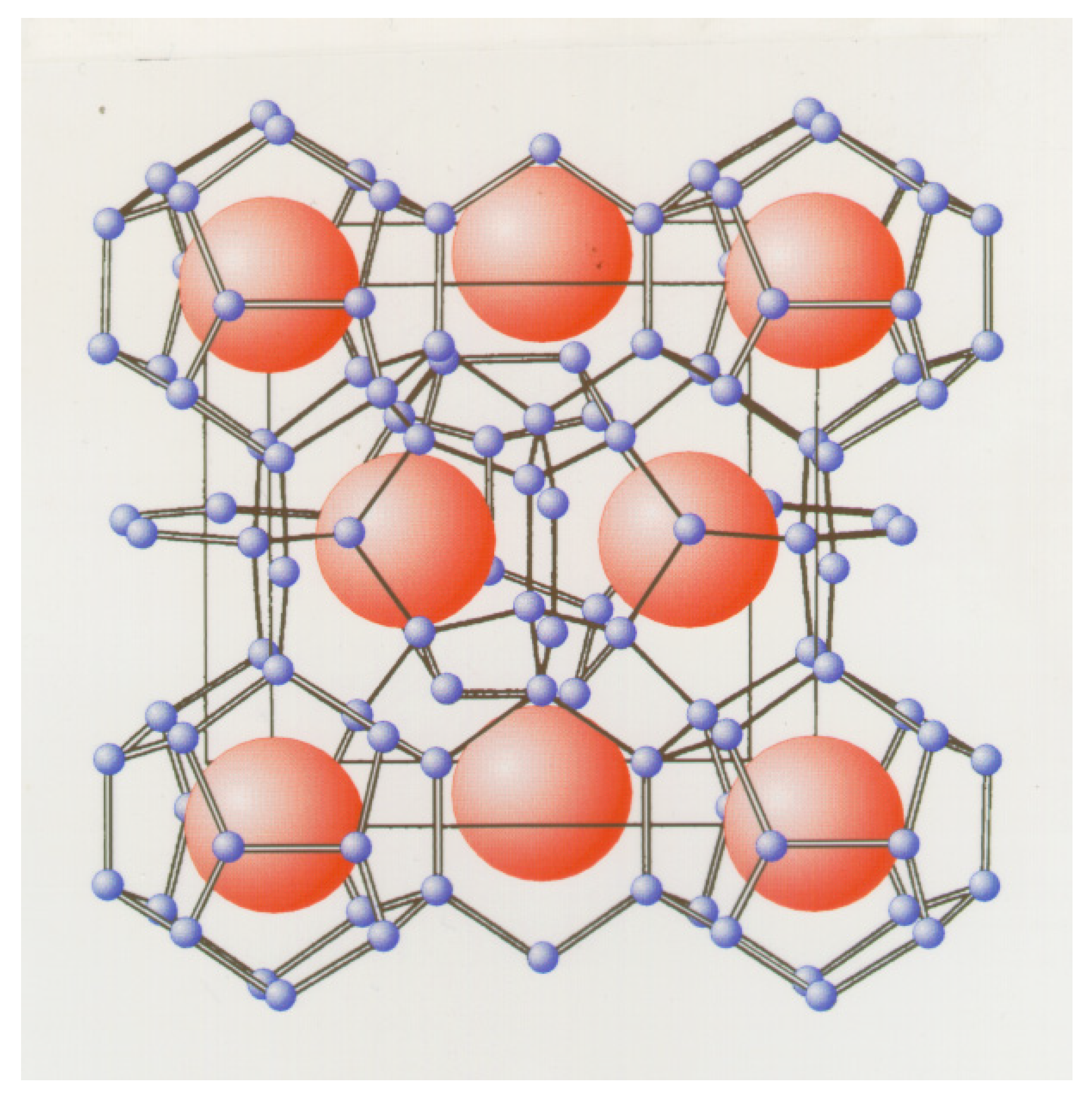
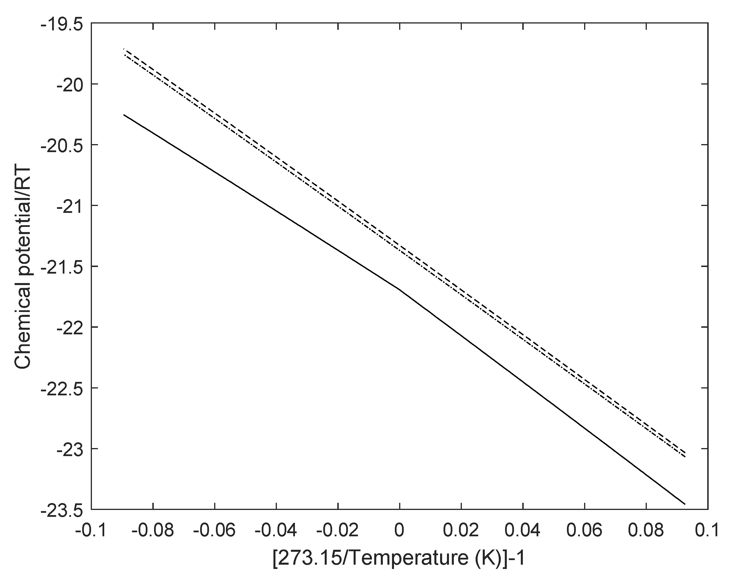
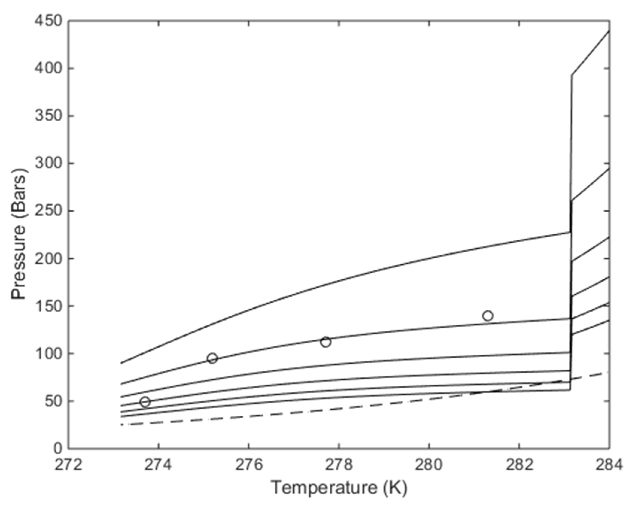
Table 1.
Parameters for dimensionless chemical potential functions in Equation (8).
| Water Phase, m | a0 | a1 |
|---|---|---|
| Empty structure I | −21.333 | −18.246 |
| Empty structure II | −21.374 | −18.186 |
| Ice (T < 273.15 K) | −21.690 | −19.051 |
| Liquid water (T > 273.15 K) | −21.690 | −16.080 |
Table 2.
Coefficients for free energy of guest type j inclusion in cavity type k.

| i | CO2 Large | CO2 Small | |
|---|---|---|---|
| T ≤ 283.14 K | T > 283.14 K | ||
| 11 | 35.49720 | 3.79330 | 22.87614 |
| 22 | −58.70762 | 1.92897 | −5.87544 |
| 33 | −54.74851 | −10.73174 | −2.41184 |
| 44 | 7.30756 | −48.69651 | −2.12052 |
| 55 | 16.55871 | 16.20157 | −5.18454 |
| 66 | 9.06319 | 0.42555 | −9.70065 |
Table 3.
Coefficients for free energy of N2 inclusion in cavity type k.

| i | N2 | |
|---|---|---|
| Large | Small | |
| 1 | 8.85531 | −143.99019 |
| 2 | 10.87598 | −95.44723 |
| 3 | 25.06545 | 4.68052 |
| 4 | 54.17078 | 59.13995 |
| 5 | 20.64268 | 109.87325 |
| 6 | −133.44618 | 113.79746 |
| 7 | −130.99357 | 149.13992 |
| 8 | −85.72083 | 139.08208 |
| 9 | −106.74770 | 153.82431 |
| 10 | −78.83698 | 141.94965 |
© 2020 by the authors. Licensee MDPI, Basel, Switzerland. This article is an open access article distributed under the terms and conditions of the Creative Commons Attribution (CC BY) license (http://creativecommons.org/licenses/by/4.0/).
Share and Cite
MDPI and ACS Style
Kvamme, B.; Zhao, J.; Wei, N.; Saeidi, N. Hydrate—A Mysterious Phase or Just Misunderstood? Energies 2020, 13, 880. https://doi.org/10.3390/en13040880
AMA Style
Kvamme B, Zhao J, Wei N, Saeidi N. Hydrate—A Mysterious Phase or Just Misunderstood? Energies. 2020; 13(4):880. https://doi.org/10.3390/en13040880
Chicago/Turabian StyleKvamme, Bjørn, Jinzhou Zhao, Na Wei, and Navid Saeidi. 2020. "Hydrate—A Mysterious Phase or Just Misunderstood?" Energies 13, no. 4: 880. https://doi.org/10.3390/en13040880
Note that from the first issue of 2016, this journal uses article numbers instead of page numbers. See further details here.