Granger Causality Network Methods for Analyzing Cross-Border Electricity Trading between Greece, Italy, and Bulgaria

Abstract

Italy, Greece, and, to a lesser degree, Bulgaria have experienced fast growth in their renewable generation capacity (RESc) over the last several years. The consequences of this fact include a decrease in spot wholesale prices in electricity markets and a significant effect on cross border trading (CBT) among neighboring interconnected countries. In this work, we empirically analyzed historical data on fundamental market variables (i.e., spot prices, load, RES generation) as well as CBT data (imports, exports, commercial schedules, net transfer capacities, etc.) on the Greek, Italian, and Bulgarian electricity markets by applying the Granger causality connectivity analysis (GCCA) approach. The aim of this analysis was to detect all possible interactions among the abovementioned variables, focusing in particular on the effects of growing shares of RES generation on the commercial electricity trading among the abovementioned countries for the period 2015–2018. The key findings of this paper are summarized as the following: The RES generation in Italy, for the period examined, drives the spot prices in Greece via commercial schedules. In addition, on average, spot price fluctuations do not affect the commercial schedules of energy trading between Greece and Bulgaria.

1. Introduction

Over the several past years, European electricity markets have gone through a process of significant developmental changes which contributed to the further liberalization of the energy sector. In addition to this, European countries are committed to reach specific targets for 2030 and 2050 regarding the percentage of renewable energy sources (RES) participation in the energy generation mix, alongside the targets set by the European Green Deal [1]. Variable energy sources (VRES), especially solar and wind, cannot produce constant power since they are highly correlated with weather conditions.

European electricity markets are becoming increasingly integrated under the target of a single European electricity market. Greece has not yet market-coupled with any of the interconnected countries, but it is expected to do so under the “European Target Model” (ETM) mechanism by June 2020. The traded energy volume appears to have a severe degree of seasonality with human activities slowing down towards summer and then increasing again, based on European electricity market reports [2]. In general, energy trading follows demand. The implemented policies led the traded energy volume within European countries to reach the 33% of the total consumption in the first quarter of 2019 which indicates a 4% increase compared to the corresponding period of the previous year [3]. Nevertheless, in the second quarter of 2019, a reduction of 14% compared to the same period of the previous year in trading volume appeared [4]. The aforementioned policy of increasing the number of market-coupled countries within Europe and hence enforcing the pan-European energy market was initially designed in order to achieve energy price convergence and thus ensuring the highest level of safety and security of supply [5].

On the other hand, European countries following the 2030 climate and energy framework have pledged to reduce the use of fossil fuels and increase RES to improve their share in the energy generation mix [6]. This has led to a remarkable increase of RES, particularly solar and wind power. The European Union has committed to obtaining 20% of the consumed energy until 2020 from RES with this percentage increasing to the 32% in 2030 [7]. These targets will be revaluated for an upward revision in 2023 [6]. By 2017, the respective percentage was 17.5% with some countries having already achieved their individual targets [8].

The increased share of RES has a direct effect on spot prices since, as investigated, it is highly correlated with solar and wind intermittent availability. In general, deployment of renewable (mainly wind and solar) generation capacity affects the dynamics of electricity spot prices in a negative way, while the opposite happens with its volatility [9,10,11]. This should be anticipated since RES are more efficient than conventional generators in terms of marginal cost, but on the other hand, they cannot guarantee a constant and secure supply, since they are highly dependent on exogenous parameters.

This combination of uncertainty and lower spot prices discourage stakeholders from investing in new capacities, either from renewables or conventional sources. However, market designs can, to some extent, smoothen the volatility of electricity prices and enhance investments [12].

In this paper, we studied the abovementioned issues by considering the interconnection of Greece with Bulgaria and Italy and the effect of one country’s intermittent generation to the other’s market clearing price and, more importantly, on their cross border trading (CBT). In addition to this, we tried to leverage the available data and detect any hidden (causal as we will mention in the results section) connections among CBT fundamentals. All the examined countries invest in VRES deployment while taking advantage of the interconnection. The level of the system marginal price (SMP) in Greece, which is consistently one of the highest in Europe, discourages new investments in energy capacity. However, the interest is high, since the Greek energy market has room for improvement, especially under the implementation of the ETM. Therefore, we believe that our work will highlight the effect of RES growth in these countries and how this contributes to the changes in Greek SMP and commercial schedules.

Currently, Greece has active electricity interconnections with Turkey, Albania, North Macedonia, Bulgaria, and Italy with the latter being the most active regarding total exchanges. In 2017, 22.72% of energy imports in Greece were from Italy, while the respective percentage of energy exports was 26.82% of the total. The total imports in Greece for 2018 were 11,223.913 MWh, and exports were 4983.061 MWh [11].

However, it should be mentioned that the above countries are connected to each other via physical interconnection and not by market coupling, hence comparison with other studies that investigate countries that are connected via market coupling might lack common ground. However, misfunctions of simple interconnection compared to market coupling can be detected.

The rest of this paper is organized as follows: A thorough literature review is presented in Section 2. Previous works on CBT using multiple models are illustrated in this section. In addition to this, detailed information on the methodology is provided. Section 3 briefly presents the market structure of the examined countries and the interconnection between policy and procedure. Section 4 and Section 5 illustrate the data (time series) we used for the completion of the current work on the preprocessing procedure, their summary statistics, and the correlations among them. The Granger causality connectivity analysis is briefly presented in Section 6. The methodology and the results exploitation as well as the data preprocessing and the model’s validation are shown in this section. Finally, the outcomes of the simulations along with a discussion are provided in Section 7 and Section 8, respectively.

2. Literature Review

Various studies have been conducted examining how the increasing penetration of renewables combined with interconnections among neighboring countries affect the dynamics of electricity spot prices domestically and cross border as well as their inter-trading commercial schedules. Since Germany is the leading country in Europe implementing renewable generation in its energy mix and one of the countries with the most cross border interconnections (CBI), it has been the center of research by the scientific community [10,13,14].

The first layer of the investigation consists of the consequences the increasing RES capacity has on the domestic SMP. Ketterer (2014) [13] used daily data on a GARCH model to examine the effect of domestic wind electricity generation on the volatility of electricity price. Specifically, the study showed that increasing wind generation reduces the price levels while at the same time increases its volatility.

In addition to the previous study, Wozabal et al. (2014) [10] using hourly data and ordinary least squares regression (OLS) showed that Intermittent Energy Sources (IES)affects SMP in a complex way. For a small to moderate quantity of IES, the price variance tends to decrease, while large quantities of IES have the opposite effect. Furthermore, in their study they highlighted some policy measures that might support variance absorbing technologies. Grid interconnections were one of the suggested measures, in the sense that they might operate as a means of ensuring the development of sufficient capacities over time.

Extensive investigation has been conducted regarding the Germany–France interconnection. German intermittent electricity generation has been proven to affect the dynamics of French spot prices. Specifically, increasing German renewable generation leads to a decrease in the level of French spot prices but has a positive effect on its volatility [12]. A step forward has been made by Haximusa (2018) [14], who showed that wind and solar generation in Germany have an ambiguous effect on the volatility of French spot prices. He considered three levels of French demand (i.e., low, medium, and high) and applied a GARCH analysis to show the effects on the spot price regarding the different demand levels. He proved that during medium and high French demands, importing energy from Germany decreases the spot price volatility, while the opposite happens when the demand is low.

Another example of strong interconnection coupled with increasing competition is the Nordic electricity market. Bask et al. (2008) [15] applied a stochastic model to generate electricity prices at Nord Pool and then used a GARCH analysis to show that prices became less sensitive to external shocks while the Nordic power market was being expanded and the degree of competition was being increased.

Denny et al. (2010) [16] investigated how the increasing penetration of wind generation affects the spot price dynamics of countries coupled to the UK and Ireland. The results indicate that increasing interconnections will reduce the level as well as the volatility of spot prices in both countries.

A paper that is very related to our work here, as far as its main topic is concerned, is the work of Zugno et al. 2013 [17], dealing with the influence of wind power generation on European cross border power flows. Wind power generation and spot price have been found to have a non-linear effect on cross border power exchange across Europe. Using Principal Component (PC) analysis (to reduce the problem’s dimensionality), cross border power exchange hourly data were used as dependent variables in local polynomial regression using the PC (extracted from the matrix of cross border flow variables) as exogenous factors. The main findings in this work were that an increase in forecasted wind power generation causes a fall in the German import of power (or rise in the export), while rising spot prices show the opposite direction. Another very significant finding was that, from a global perspective, variations in wind power generation in Germany had significant effects on power flows in Europe. More specifically, import and export patterns were largely altered and loop flows were originated. The abovementioned paper was a data-driven research study made possible due to the availability of data on wind power generation, consumption, and power flows provided by the European Network of Transmission System Operators for Electricity (ENTSO-E). In general, the higher the wind power penetration in Germany, the more this country exports to its direct neighbors to the South. Also, it appears that there is a loop flow in the power transit from Germany to Switzerland via Austria, since the flow from Austria to Switzerland is positively correlated with German wind power generation. In our work, presented in this paper, we tried to detect similar interactions using, however, Granger causality analysis, on the CBT between Italy–Greece–Bulgaria.

In the present work, we have applied Granger causality (GC) on hourly data extracted by ENTSO-E database for four years (2015–2018). To the best of our knowledge, the cross-border electricity exchange among the abovementioned countries has not yet been investigated and, hence, our work appears to provide a valuable contribution to the scientific community. Another aspect of our work is that we examined how a country’s spot price (e.g., Greece) and commercial (trading) schedule was affected by VRES generation in a neighboring country (e.g., Italy) without the existence of a market coupling policy.

Granger causality, an established time series technique, was used to analyze the interactions (“cause and effects”) of a representative sample of 13 European electricity spot prices for the period 2007–2012 [18]. The study applied GC via network theory and provided inferences regarding the European electricity network’s state and dynamic evolution over time, therefore assessing spot price convergence and “quality” of market coupling. The causal interactions among European electricity spot prices were modeled as a connectivity network on which the spot prices constituted the nodes of the network, while the links corresponded to the significant influences among relative pair-wise price changes.

One of the early applications of causal flow modeling in electricity markets is the work by Park et al. (2006) [19], in which the authors used advanced techniques in causal analysis (vector autoregressive (VAR), vector error correction model (VECM), and directed acyclic graphs (DAGs)) to find the dynamic relationships between electricity spot prices and the prices of major electricity-generation fuel sources (i.e., oil, gas, and coal prices) in US electricity spot markets.

A multivariate version of GC was used in a paper by Narayan et al. (2009) [20] to examine the causal relationships between electricity consumption, exports and gross domestic product for a panel of Middle Eastern countries.

In their causal modeling and inference for electricity markets, Ferkingstad et al. (2011) [21] used a combination of VAR, VECM, and a linear non-Gaussian acyclic model (LiNGAM) which they call time-lagged causal flow, a concept very close to the GC. They applied their hybrid model to weekly Nordic and German electricity prices, using oil, gas, and coal prices with German wind power and Nordic water reservoir levels as exogenous. They showed that, in contemporaneous time, Nordic and German spot prices were interlinked through gas prices.

A combination of out-of-sample Granger causality tests and DAGs were also used by Yang and Zhao (2014) [22] to investigate the temporal linkages among economic growth, energy consumption, and carbon emissions in India.

The methodology applied in this work, referred onwards as Granger causality connectivity analysis (GCCA), is based on modern network theory, an efficient approach to characterizing connecting systems [23]. Our purpose was to study the dynamic evolution of the network and the nodes which included the following criteria of three countries: the spot prices; imports–exports, the demand (load), the VRES generation; and the commercial schedules of CBT. This study will inform how the spot prices of the above countries are influenced by their own interactions as well as by the interactions of the other variables. Based on the results of this study, we will be able to draw conclusions regarding the cross-border trading development of this “peripheral” sub-system of the European electricity system.

The identification of directed operation connectivity among the components of a system is a challenging work. The GCCA is a powerful tool in detecting such connectivities in complex systems such as an electricity market. Granger Causality is a way to investigate “causality” between two variables, a probabilistic account of causality, and a concept closely related to the idea of cause and effect but not the same. GC allows one to know which particular variable comes before another in a time series but does not describe a causal link in the true sense. In Econometrics, “cause” is actually realized as “Granger cause”.

The most recent approach to complex systems is the contemporary network theory, originating from the small world theory of Watt and Strogatz (1988) [24], as well as its scale-free “version” of Barabasi and Albert (1999) [25]. Recently, a large number of papers has focused on various applications of complex networks [26]. We applied this fascinating approach to the CBET among three neighboring countries to extract valuable information regarding their interactions. The results are expected to be useful in policy design among other areas. All calculations in this paper were based on the theoretical approach to GCCA presented in the work of Seth (2008, 2010 2014) [27,28,29] and implemented by using his toolbox run on MATLAB (ver.2019a, The MathWorks Inc., Natick, MA, USA).

A review paper presenting the application of GC in energy economics research is given by Narayan and Sangth (2014) [20]. The examination of causal relationships between the electricity consumption and economic growth using linear and non-linear GC tests in the case of Turkey is presented in the paper by Nazlioglou et al. (2014) [30]. The tests reveal a bi-directional GC in both the short and long run between the electricity consumption and economic growth in Turkey. The relationship between economic output and energy use is also the focus of a work by Brun et al. (2014) [31]. Woo et al. (2006) [32] applied a Granger instantaneous causality test in order to examine the potential causal relationships between wholesale electricity and natural gas prices in California, revealing bi-directional relationships between these two markets [32]. An in-depth analysis of the causal relationships in oil markets globally is given in a thesis work by Antoniadou (2015) [33]. In this work, the GC and the Toda–Yamamoto approaches were applied, revealing that the causality between crude oil prices and natural gas prices is not bi-directional, since only crude oil prices Granger causes natural gas prices. The relationship between investor attention and crude oil prices is examined by the paper of Li et al. (2019) [34]. Using the Google search volume index (GSVI) that “captures” investor attention, the author used linear and non-linear GC tests. The results show that a bi-directional GC exists only between WTI future crude oil returns and investor attention.

The latent volatility GC for four renewables energy exchanged traded funds (ETFs) and crude oil ETF (USO) were examined in a work by Chang et al. [35]. The empirical results showed that there are significant positive latent volatility GC relationships between solar, wind, nuclear, and crude oil ETFs as well as significant volatility spillovers shocks for renewable energy ETFs. Using a GC in quantiles analysis (evaluating causal relations in each quantile of the distribution), they succeeded in discriminating between causality affecting the median and the tails of the conditional distribution and provided evidence for the existence of a bi-directional causality between changes in RES consumption and economic growth using RES consumption, oil prices, and economic activity data in the US (July 1989 to July 2016).

The GC test was also used in analyzing spillover effect of oil and natural gas prices between emerging and developed countries in a paper by Zhong et al. (2019) [36]. The main findings were that oil and natural gas markets have significant GC and that emerging markets have a strong impact on many developed markets regarding returns and volatility spillover systems.

A combination of GC test and the (recently developed) cross-quantilogram was used on crude oil, natural gas, heating oil, electricity, and gasoline market data to evaluate their directional predictability in a work by Scarcioffolo et al. (2019) [37]. They found no strong evidence to support the decoupling between crude oil and natural gas markets. Natural gas and heating oil were found to be strongly linked across all quantiles.

3. Wholesale Electricity Markets: The Case of Greek, Italian, Iberian, French, and Bulgarian Markets

3.1. The Greek Market

Greece’s liberalized electricity market was established according to European Directive 96/92/EC. The Greek Wholesale Electricity Market (GEM) currently operates as a day ahead mandatory pool which is based on an optimization algorithm for both energy and ancillary services [38] taking into account the following:

• Predictions of demand (on different time scales);
• Offers from generators and bids from suppliers;
• Units’ availability and technical constraints (min, max, ramp up, ramp down);
• Must-run production (e.g., hydro power plants);
• Commercial schedules of the interconnections.

Greek Wholesale Energy Market GEM is in a transitional period towards its final design, namely, ETM where both an intra-day market and a balancing market are expected to operate in order to enhance GEM’s liquidity and efficiency. More specifically, the new regulatory framework for the ETM makes provisions for a day-ahead and intra-day market managed by Hellenic Energy Exchange S.A. (Athens, Greece) and a balancing market managed by Greece’s Transmission System Operator (IPTO) (Athens, Greece). The new day-ahead market will be a semi-compulsory market, where orders should cover the availability and should be compatible with Price Coupling of Regions algorithm (PCR EUPHEMIA) standards, and the biddings will be on a physical asset basis except RES which could be on a portfolio basis. There are also provisions for exchange-based futures and over-the-counter (OTC) contract limits on the volumes.

3.2. The Italian Market

In Italy, Gestore del Mercato Elettrico (GME) is responsible for the operation of the power market as well as gas and environmental ones. Gestore del Mercato Elettrico runs under the framework of the Italian Regulatory Authority (ARERA) which sets the rules and activities of the abovementioned sectors. The Italian Wholesale Electricity Market essentially runs on the Italian Power Exchange (IPEX), where producers and suppliers trade blocks of energy. More specifically, GME operates a day-ahead market (MGP) based on auctions, an intra-day auction market (MI), a forward market (MTE), and a market (MPEG) for continuous trading of energy daily products. Moreover, it operates on behalf of TERNA which is the Italian Transmission System Operator the Ancillary Services Market (MSD) while at the same time issues the OTC transactions (PCE).

Italy is divided into six zonal markets based on geographical criteria. These are Northern Italy (NORD), Central Northern Italy (CNOR), Central Southern Italy (CSUD), Southern Italy (SUD), the Sicily (SICI), and Sardinia (SARD). Greece is connected to SUD, which is the South part of the Italian electricity system. The zonal price, in the case of no congestion, is unique and is the interception of the aggregated demand and supply curves which are calculated after an algorithmic procedure. In the case of congestion, the market is split into the four aforementioned regions, and the system calculates different price equilibriums. The national unique price (PUN), which is the consumer price, is the weighted average of the individual zonal prices [38].

3.3. The Iberian and French Electricity Markets

Italy has already established a market coupling relationship with France and hence with the Iberian wholesale electricity market. The Iberian wholesale electricity market MIBEL, is a joint wholesale electricity market which comprises Spain and Portugal [39]. OMI-Polo Español S.A. (OMIE) belongs to the Iberian Market Operator business group, and it is subject to the rules and regulatory framework governing Spain’s electricity sector [40]. The Iberian Wholesale Electricity Market is composed of an intra-day market and a day-ahead market producing a common spot price for both Spain and Portugal, unless there is a violation in the interconnection capacity between them; in such a case, a market splitting mechanism is activated which results in different prices for both countries. The Spanish Transmission System Operator (REE) and the Portuguese one (REN) are responsible for the technical implementation of the daily schedules. Following the gate closure, six intra-day market sessions are held four hours ahead of the physical delivery [41].

The French wholesale electricity market plays a key role in the French power system by allowing the balance between supply and demand. Most of the electricity (95%) injected into the French power system comes from nuclear and other sources (hydro, gas, coal, renewable energy sources) with a small percentage (5%) covered from imports [42]. Electricity products of the French Wholesale Electricity Market are traded on power exchanges or over the counter (OTC) via brokers or through bilateral agreements between the involved parties. The spot products are daily (day-ahead) or weekend products delivered at base load hours or during peak hours (from 8 a.m. to 8 p.m. for the working days) [43]. The abovementioned products are available on an hour or half-hour basis or as complex blocks covering several hours. The spot price of the French Wholesale Electricity Market is the price of the day-ahead market which is run on the European Power Exchange (EPEX SPOT) [44].

France is connected to the Central European System through its six interconnection lines to England, Belgium, Germany, Switzerland, Italy, and Spain. Currently the interconnection capacity between Spain and France is approximately 5% of its installed capacity which is far below the EU targets for interconnections; this limit has been set at 15% for 2030 at the EU level [45]. At the moment, the planned interconnections between France and Spain through the Gulf of Bizkaia is under consultation; this project has been characterized as a project of common interest with an interconnection capacity of 5000 MW. The latter is expected to be in operation between 2024–2025 [46,47].

3.4. The Bulgarian Market

The Bulgarian electricity market operates under the command of the Independent Bulgarian Energy Exchange (IBEX) which was established in 2014 as a 100% subsidiary of Bulgarian Energy Holding and is among the last countries introducing such an exchange market. A major change that was introduced by IBEX was the establishment of an organized day-ahead market, in 2016, to replace the pre-existing model.

Currently, IBEX operates three trading platforms: a day-ahead market, and intra-day market, and a centralized market for bilateral contracts; it is mandatory for generators with an installed capacity of 1 MW or more to sell their electricity through IBEX.

The electricity market consists of two segments.

• Regulated Market

Prices are set by the regulator (Energy and Water Regulatory Commission) and consumers are supplied based on territory. This segment includes households and small businesses connected to the low voltage distribution network.

• Free (Liberalized) Market

Electricity is freely negotiated and bought by suppliers and consumers directly from the electricity generators or via IBEX. According to the last amendment (May 2019), all RES and co-generation power plants with an installed capacity of 1 MW or more have the obligation to sell their electricity only via the power exchange.

3.5. Markets Comparison

One of the outmost criteria to measure a market’s concentration and hence define its competitiveness is the Herfindahl–Hirschman index (HHI). Even though in various cases it fails to consider the complexities of various markets, it remains a reliable index. Specifically, regarding the EU energy markets, the European Commission has set the limits for the HHI as shown in

Table 1. Herfindahl–Hirschman index (HHI) in the power generation ‘’market’’ of the analyzed electricity markets for 2015-2018 as depicted in the national reports of regulators sent to the European Commission (EC).

Year	HHI (Greek Market)	HHI (Italian Market)	HHI (Bulgarian Market)
2015	6804 (vhc *)	882 (d *)
2016	6423 (vhc *)	881 (d *)
2017	6357 (vhc *)	755 (d *)
2018	5627 (vhc *)	730 (d *)	>4700 (hc *)
Mean (2015–2018)	6302 (vhc *)	812 (d *)	>4700 (hc *)

* Legend (according to the European Commission 2014 [46]): vhc = very high concentration (HHI > 5000), hc = high concentration (1800 < HHI < 5000), mc = moderate concentration (1000 < HHI < 1800), d = deconcentration (HHI < 1000).

[46].

Figure 1 illustrates the energy generation mix in 2018 for the examined countries.

From the energy generation mix above, we can observe that Bulgaria was primarily dependent on nuclear power (36%) as a source of energy, which does not appear in either the Greek generation mix nor in the Italian, and on lignite (40%). On the other hand, Italy devoted 45% of its generation mix to natural gas, and the corresponding amounts for Greece and Bulgaria were 28% and 4%, respectively.

The common element that is being illustrated is the share of hydro in the examined countries’ energy mix. Specifically, hydro in Greece accounts for 18%, in Italy for 17%, and Bulgaria for 13% of the total energy generation. Finally, Greece appears to have the highest percentage of RES generation in the energy mix (31%), followed by Italy (23%) and Bulgaria (6%).

3.6. Cross Border Trade in Electricity

The future “architecture” of the European CBT will be based on capacity allocation and congestion management (CACM). According to CACM, all TSOs are required to develop deliverables towards implementing the markets coupling, the so-called single intra-day (SIDC) and single day-ahead coupling (SDAC) [50]. The regulation also outlines the methods for calculating how much capacity the participants in the market can use on cross border lines without putting the system at risk. Also, the document harmonizes cross border market operations in Europe in order to enhance the competition and the integration of renewables.

The SIDC creates a single EU cross-zonal intra-day electricity market, in which buyers and sellers of energy cooperate to trade electricity continuously on the day the energy is needed. The SIDC enhances the efficiency of intra-day trading across Europe by competition promotion, liquidity increase (facilitating the mechanism of buying and selling without affecting the price), making the sharing of energy generation resources easier [51].

The SIDC is implemented in three phases or waves. In the first wave, 14 countries went live in June 2018, in the second wave 7 countries, including Bulgaria, went live in November 2019. Italy and Greece will be included in the third wave, foreseen for Quarter 4 of 2020 [52].

The SDAC is the pan-European single day-ahead coupling serving 27 countries (at the time of the writing of this paper). Under this agreement, 33 TSOs and 16 nominated market electricity operators (NEMOs) will cooperate. The SDAC uses (PCR EUPHEMIA), that calculates, across Europe, electricity spot prices and does not allocate implicitly the auction-based cross border capacity [53]. According to the Agency for the Cooperation of Energy Regulators (ACER), SDAC has improved the level of efficiency regarding the usage of the interconnections from 60% in 2010 to 87% in 2018 [54].

On the 1st of October 2018 (first delivery date of the projects related to SDAC), the Germany–Austria bidding zone split was successfully implemented. In South East Europe (SEE), the target times for the bidding zone borders adhering to CACM are as follows [52]:

• Bulgaria–Greece: to be defined;
• Greece–Italy: Quarter 4, 2020.

The electricity trade can be unidirectional or bidirectional over long time horizons. Electricity flows in either direction due to the demand changes in both countries, for example, when the latter is not perfectly correlated due to the different seasonal or diurnal patterns.

The correlation coefficient between Greece’s and Italy’s forecasted load was 0.524 and statistically significant (so the loads were not perfectly correlated, indicating the existence of strong bidirectionality of CBT).

According to Antweiler [55], higher correlations diminish trade, a very essential finding, since if demand is strongly correlated between two countries, they will both have high and low demand simultaneously, allowing a limited space for additional trade. Another very significant finding in Reference [55] is that the intensity of cross-border electricity trading increases along with the coefficient of variation (cost/total demand) and that the difference or dissimilarity in the size of the countries (e.g., Italy versus Greece) encourages more trade.

A top priority for the European Commission is the harmonization and integration of national electricity markets to a single pan-European market [5]. Energy policy, however, remains strongly a tool of national sovereignty which means that a greater level of integration corresponds to the fact that unilateral national policies can impact interconnected markets.

In this work, we investigated the impact of interconnections on the expansion of renewables promoted by fixed-in tariffs and (unlimited) priority on DA-prices between Italy, Greece, and Bulgaria, as they are revealed through CBT. The contribution of the specific hub-selection lies on the lack of market coupling among the examined countries, and hence the CBT operates as a simple interconnection. It would be of high importance to identify any differences between market-coupled countries’ CBT and the specific work.

3.7. Greece’s Imports and Exports

Greece relies heavily on interconnections to meet the demand. This is due to the fact of high wholesale electricity prices which remain high despite the penetration of RES into the system. Moreover, due to the economic recession investment in RES (which, in general, lowers spot prices) had been discouraged.

The average relative margin available for cross zonal trade (MACZT) between 2016 and 2018, as calculated by ACER [54], for Greece and Italy, relative to maximum admissible active power flow (Fmax), set to at least 70% by the clean energy package (CEP), is almost 100%, and the percentage of hours when MACZT is at least 70% for the GR–IT border is also almost 100%.

According to the same report [54], for the border between Bulgaria and Greece, the average DA price differential (€/MWh) and average of absolute DA price differential (€/MWh) during the period 2016–2018 is as follows (

Table 2. Average and average absolute DA price differential for the Bulgaria–Greece border.

Year	Average DA Price Differential	Average Absolute DA Price Differential
2016	−6.0	14.6
2017	14.6	19.8
218	−20.5	24.2
2016–2018	−4.0	19.5

).

In 2018, the annual average DA prices in Greece (60.4 €/MWh) and Italy (62.04 €/MWh) were among the highest in European bidding zones, whereas Bulgaria’s DA prices were among the lowest (39.89 €/MWh). This difference in DA prices justifies the fact that during this specific period, Greece was a major exporter, as shown in Figure 2, in all neighboring countries except Italy.

Figure 3 illustrates the monthly amount of energy trading between Greece and all the interconnected countries for the examined period (2015–2018).

From Figure 3 we observed a reduction in the difference between imports and exports (interconnection balance). It was continuously positive, which means that Greece exported less energy than it imported (it is a net importer) during the whole period between 2015 and 2018.

As far as the rate of implementation of the ETM for DA markets is concerned, significant progress has been made in recent years. The ETM foresees a single DA coupling, enabling the efficient use of cross-zonal capacity in the “right economic flow (direction)” (from low to high price), when there is a price differential across a bidding zone border. The level of efficient use of interconnectors in the DA market timeframe and the estimated social welfare gains still to be obtained, from extending DA market coupling per border, are the two indicators that illustrate the progress toward ETM.

The estimated social welfare gains, still to be obtained, from further extending DA market coupling in the borders of Greece–Italy and Greece–Bulgaria, during the period between 2017 and 2018, as calculated by ACER [56] are illustrated in

Table 3. The estimated social welfare gains from further extending Day Ahead (DA) market coupling in Greece and Italian/Bulgarian borders.

Border	2017	2018
GR–IT	6	10
BG–GR	22.5	18.5

.

Historically, Greek Wholesale Electricity Prices (SMPs) were driven by the low prices of fossil fuels and more specifically from the lignite ones. The Green Deal alongside climate change awareness made the EU impose stricter rules for CO₂ emissions. The 2030 and 2050 emission targets (90% reduction compared to 1990 EU levels) led to higher prices for CO₂ emission rights which, in turn, had a dramatic impact on lignite prices. The latter seriously affected the GEM, since gas prices are now compared to lignite prices which, in turn, incurs higher wholesale electricity prices according to the merit order mechanism. Also, even though Greece has already achieved the EU targets for RES penetration levels by 2020, this is not mirrored in market prices due mostly to the financial crisis of 2011 but also to the low volatility and liquidity of GEM.

3.7.1. Joint Allocation Office (JAO)

The Joint Allocation Office (JAO) is a joint service company that consists of 22 TSOs in 19 countries and facilitates the electricity market by organizing auctions for cross border transmission capacity. It was created in June 2015 and was the result of the merge between the Central Allocation Office (CAO) and ASC.EU S.A. located in Germany and Luxembourg respectively, the two former regional allocation offices for cross border transmission capacities. On the 1st of October 2018, JAO became the Single Allocation Platform (SAP) of forward capacity for all European TSOs, operating in accordance with EU legal rules. Currently, JAO performs long- and short-term auctions of transmission capacity and is the duty of the national regulatory authorities to decide which auction should be performed.

3.7.2. Greece–Italy (GR–IT) Interconnection

Currently, Greece and Italy operate as two separate electricity markets, while no market coupling has been applied.

Before the annual and monthly capacity allocation process, IPTO (ADMIE) calculates the GR–IT Net Transmission Capacity (NTC) and agrees on it with TERNA. The final NTC values are stored in the system and then communicated via email to JAO. After receiving the NTC values, JAO is responsible for the annual and monthly transmission rights allocation on GR–IT border. Joint Allocation Office (JAO) performs the auction and informs IPTO and TERNA of the capacity auction outcome.

Two days before the scheduling day (until 12:30 CET), IPTO receives from JAO the annual and monthly final capacity right documents which are aggregated into the long-term capacity rights.

The values of daily ATC and relative data are submitted by ADMIE and TERNA to JAO every day (until 09:30 CET). Once the daily auctions are calculated, they are sent by JAO to ADMIE and TERNA.

After having received the capacity right document, IPTO interacts with the capacity holders or their counterparties who inform IPTO of the capacity they are going to use, based on their capacity rights documents (long term or short term).

The day-ahead scheduling process, performed by IPTO, includes two phases of nominations, submission and matching.

The long-term (LT) phase: until 08:30 CET, capacity holders submit their nominations based on long-term rights. Consequently, IPTO and TERNA exchange and match the LT nominations until 09:00 CET. In the case of a mismatch, the export value prevail rule is applied.

The remaining capacity (non-nominated LT capacity rights), until the NTC of the GR–IT interconnection, comprises the offered capacity for daily auctions (performed by JAO). The IPTO sends both LT and ST capacity rights to ENEX which is the NEMO for the Greek DAM. The SMP of the Greek DAM is the hourly solution of the algorithm of the daily co-optimization of the energy production bids (taking into account the techno-economic constraints of the plants) as well as the energy bids of importers and exporters and the Load declaration of load representatives. The total commercial schedules are determined up to 99% by the Greek DAM clearing, and they have a causal relationship with the price difference between Greek DAM and South Italy marginal prices.

The short-term phase: until 14:30 CET, capacity holders submit their nominations based on both LT and ST rights. Both IPTO and TERNA exchange and match the LT and ST nominations until 15:35 CET. In the case of a mismatch, the minimum value prevail rule is applied.

3.7.3. Greece–Bulgaria (GR–BG) Interconnection

The interconnection between Greece and Bulgaria operates more or less similarly to the GR–IT one, with no market coupling and through the JAO platform. The responsible party for the Bulgarian side is ESO (the Bulgarian system operator).

The auctions between Greece and Bulgaria are bidirectional and are separated to:

• Daily auctions;
• Monthly auctions;
• Yearly auctions.

The NTCs, which are the auctioning basis, are agreed to between IPTO and ESO. Afterwards, the NTCs and ATCs for each interconnection and direction are published on the auction websites. If there is a change to the ATCs regarding the monthly auctions, users can be informed timely regarding the relevant auction website.

4. Data and Preprocessing

We focused on the Italian, Greek, and Bulgarian electricity markets, their actual and forecasted solar and wind power productions, demands (loads), DA-prices (spot or wholesale prices), and finally their commercial schedules and transfer capacities of cross-border trading with their interconnected countries. Below, we may refer to them as cross-border trading fundamentals (CBTFs).

Table 4. Data Overview.

Data (Variable)	Description	Unit of Measurement	Resolution
D1	Values of forecasted solar production in the South Italian region that is connected to Greece	MWh	Daily
D2	Values of forecasted wind production in the South Italian region that is connected to Greece	MWh	Daily
D3	Values of forecasted Solar production in Greece	MWh	Daily
D4	Values of forecasted Wind production in Greece	MWh	Daily
D7	Total forecasted demand (load) in Italy	MWh	Daily
D9	Total forecasted demand (load) in Greece	MWh	Daily
D11	Wholesale electricity price in the South Italy region that is connected to Greece	€/MWh	Daily
D12	Wholesale electricity price in Greece	€/MWh	Daily
D13	Total commercial schedule from Italy to Greece 1	MW	Daily
D14	Total commercial schedule from Greece to Italy	MW	Daily
D15	NTC from Greece to Italy 2	MW	Daily
D16	NTC from Italy to Greece	MW	Daily
D17	Values of forecasted solar production in Bulgaria	MWh	Daily
D18	Values of forecasted wind production in Bulgaria	MWh	Daily
D21	Wholesale electricity price in Bulgaria	lev/MWh	Daily
D22	Total commercial schedule from Bulgaria to Greece	MW	Daily
D23	Total commercial schedule from Greece to Bulgaria	MW	Daily
D24	Total forecasted demand (load) in Bulgaria	MWh	Daily

¹ Total commercial schedule is the summation of all the agreed transactions for the delivery and receipt of power and energy among the traders in the interconnection. That schedules are also agreed to by the TSO of the two control areas. ² Transfer capacity is the allocated through auctions transfer ability to traders that allows them to exchange electricity among geographic areas for each market time unit and for a given direction.

below contains the description of the data which consists of hourly observations, converted to daily values (average of 24 hourly values), covering the period 2015 to 2018 (1460 data points).

Regarding Bulgaria, there were no available data for the DA price (D21) before 2017 which meant that in the examined cases (study A and C) of this work, which included the specific variable, we limited the data range to the years 2017 to 2018 (725 data points).

In general, we used data for the South Italy region (SUD) which connects to Greece. However, when it came to Load Forecasted, we decided that it was more accurate to use the Total Load Forecasted and not the South one. This decision was based on the procedure IPEX follows to determine the PUN, in which the Load is considered as aggregated for the whole Italy and is not split into zonal regions. Moreover, the total load forecasted in Italy is highly correlated to the load forecasted in South Italy (0.70), so we can safely use the total demand.

Hence, in the forecasted load time series for both Greece and Italy (D7 and D9), we considered in all our calculations the total forecasted load in the Italian and Greek markets.

Testing Examined Time Series for Stationarity

Since the primary precondition for Granger causality analysis is that the variables must be covariance stationary (CS), also known as weak or wide-sense stationarity, we tested our data for stationarity. Augmented Dickey–Fuller (ADF) and Kwiatkowski–Phillips–Schmidt–Shin (KPSS) tests were performed for testing the null hypothesis that the examined series had unit roots which indicates stationarity or trend stationarity.

Since we used two sets of data (2015 to 2018 and 2017 to 2018 to incorporate the Bulgarian data), the tests were performed for each one of the time series and for both data sets.

Table 5. Augmented Dickey-Fuller (ADF) and Kwiatkowski–Phillips–Schmidt–Shin (KPSS) stationarity test results.

Data (Variable)	ADF		KPSS
	2015 to 2018 (1460 Data Points)	2017 to 2018 (725 Data Points)	2015 to 2018 (1460 Data Points)	2017 to 2018 (725 Data Points)
D1	Stationary	Stationary	Stationary	Stationary
D2	Stationary	Stationary	Stationary	Stationary
D3	Stationary	Stationary	Stationary	Stationary
D4	Stationary	Stationary	Stationary	Stationary
D7	Stationary	Stationary	Stationary	Stationary
D9	Stationary	Non-Stationary	Stationary	Stationary
D11	Stationary	Stationary	Non-Stationary	Stationary
D12	Stationary	Stationary	Non-Stationary	Stationary
D13	Stationary	Stationary	Stationary	Stationary
D14	Stationary	Stationary	Stationary	Stationary
D15	Stationary	Non-Stationary	Stationary	Stationary
D16	Stationary	Non-Stationary	Stationary	Stationary
D17	Stationary	Stationary	Stationary	Stationary
D18	Stationary	Stationary	Stationary	Stationary
D21	N/A	Stationary	N/A	Non-Stationary
D22	Stationary	Stationary	Stationary	Stationary
D23	Stationary	Stationary	Stationary	Stationary
D24	Non-Stationary	Non-Stationary	Stationary	Stationary

illustrates the tests results for the acceptance or not of the null hypothesis. Rejection of the null hypothesis indicates data stationarity, while the inability to reject it indicates non-stationarity.

The ADF unit root test did not reject the null hypothesis for D24 for the whole series and for D9, D15, D16, and D24 for the reduced data series scenario. On the other hand, KPSS test indicates that D11 and D12 were not trend stationary when the whole series scenario was examined and D21 when the reduced series scenario was examined.

Therefore, for the abovementioned time series, we took their first difference to make them stationary. Then, we performed the tests again and all series appeared to be stationary and trend stationary.

To continue further with our research, we defined three studies (models) in order to find the best models to test the Granger causality of cross-border trading among the examined countries. Our aim was to conduct an analysis for all the possible combinations, hence we separated the model structure as follows:

• Study A contained variables of the three countries, treating them as consisting of a “whole” system (although Bulgaria is not directly connected to Italy), in an effort to identify any connection and interaction as a system, including “pass-through” or “hidden” causalities (transit flows);
• Study B contained variables of Greece and Italy;
• Study C contained variables of Greece and Bulgaria.

Table 6. The case studies and the variables that were included ¹.

Model	D1	D2	D3	D4	D7	D9	D11	D12	D13	D14	D15	D16	D17	D18	D21	D22	D23	D24
A	1	2	3	4	5	6	7	8	9	10	11	12	13	14	15	16	17	18
B	1	2	3	4	5	6	7	8	9	10	11	12
C			1	2		3		4					5	6	7	8	9	10

¹ The numbers below each time series indicate the corresponding node of the specific variable to the Granger causality connectivity analysis model.

shows all the variables (or nodes in the network) and the corresponding studies (models) they were included as an input.

5. Summary Statistics

5.1. Summary Statistics

Since Granger causality Analysis is a multivariate (MVAR) method and since all MVAR methods rely heavily on the assumption of normality or near-normality which is often hard to achieve in practice, we proceed in presenting summary statistics of all variables, focusing on normality aspects. The results are illustrated in

Table 7. Summary statistics.

Time Series	N	Minimum	Maximum	Mean	SD	Skewness	Kurtosis	JB Test (p-Value)
D1	1460	36.44	875.84	470.62	192.15	−0.233	1.938	81.86 (0.00)
D2	1460	20.68	3165.36	800.64	582.93	1.077	3.794	320.61 (0.00)
D3	1460	47.36	838.60	391.42	145.73	−0.336	1.988	89.74 (0.00)
D4	1460	76.40	1671.20	516.04	320.10	0.839	3.056	171.66 (0.00)
D7	1460	20,687.76	46,082.68	33,032.04	4647.46	−0.370	2.496	48.82 (0.00)
D9	1460	4060.80	8210.96	5865.18	713.22	0.482	2.627	64.87 (0.00)
D11	1460	20.07	127.30	49.72	11.47	0.779	4.978	385.58 (0.00)
D12	1460	26.91	111.40	52.41	10.63	1.121	5.365	645.96 (0.00)
D13	1460	0.00	530.40	223.52	181.02	−0.005	1.448	146.44 (0.00)
D14	1460	0.00	531.72	122.40	148.53	1.243	3.275	380.84 (0.00)
D15	1460	0.00	500.00	350.78	223.41	−0.871	1.809	271.02 (0.00)
D16	1460	0.00	500.00	351.34	223.25	−0.878	1.819	272.18 (0.00)
D17	1460	0.00	336.04	151.95	78.47	−0.016	1.913	71.98 (0.00)
D18	1460	1.92	645.04	184.43	139.82	0.983	3.251	239.15 (0.00)
D21 1	728	6.96	157.2	39.8	13.8	2.107	13.49	3864 (0.00)
D22	1460	0.00	700.00	450.60	144.32	−0.617	3.783	130.04 (0.00)
D23	1460	0.00	529.84	23.26	51.14	3.598	19.971	20,669.56 (0.00)
D24	1460	3160.84	6756.96	4321.93	694.95	0.916	3.022	204.23 (0.00)

¹ We converted Bulgarian lev to euros taking an exchange rate of 1 euro = 0.511 lev.

.

As illustrated in Table 7, none of the examined time series follow normal distribution. Some variables that worth highlighting regarding their skewness values are D2, D12, D14, D21, and D23 whose value appears to be higher than 1, which indicates strong positive skewness and hence data concentration to the right tail (maximum) of the distribution. This was anticipated for the wind generation (D2), since the specific variable was highly stochastic. However, regarding DA prices in Greece and Bulgaria (D12 and D21, respectively), the high value of skewness revealed a difficulty in the forecasting model construction. The same happens with the commercial schedules from Greece to Italy and to Bulgaria (D14 and D23). The contribution of this work is to provide a way of enhancing the forecasting by revealing and indicating any causal connections among CBTF.

Furthermore, from Table 7 we observe that all the variables appeared to have values of kurtosis close to three which was our benchmark of normality, except for D11, D12, D21, and D23. This indicates that the degree of uncertainty in the specific time series (DA prices) was high which contributes more to the difficulty of prediction.

The turnover (“liquidity”) of the South Italy electricity market was much smaller than the turnover of the Greek Market. Thus, prices of South Italy zone are more volatile than those at Greece. As illustrated in Table 7 the maximum price at South Italy was 127.30 €/MWh, and the standard deviation was 11.5 €/MWh (mean value 49.72 €/MWh). In Greece, the maximum price was111.4 €/MWh, and standard deviation was 10.63 €/MWh (mean value 52.41 €/MWh).

Finally, observing the Jarque–Bera (JB) test results, we see that none of the examined series were normally distributed, which means that we need to further analyze the data and apply decomposing methods. It is worth mentioning the corresponding value of the JB test for the Bulgarian DA price and the commercial schedule from Greece to Bulgaria (D21 and D23, respectively) which were extremely high, revealing a deviation from the normal distribution.

5.2. Correlation Coefficients

In order to have a “rough insight” into how the variables were interrelated or interacted with each other, we observed their correlation coefficients matrix. However, GC is actually a much more powerful tool to reveal any hidden causality, both in magnitude and direction.

The following tables (

Table 8. Correlation Matrix: Greece–Italy interconnection (2015–2018).

Time Series	D1	D2	D3	D4	D7	D9	D11	D12	D13	D14	D15	D16
D1	1
D2	−0.241	1
D3	0.824	−0.301	1
D4	−0.195	0.271	−0.276	1
D7	−0.030	−0.029	−0.040	0.056	1
D9	−0.050	0.014	−0.022	0.078	0.526	1
D11	0.029	−0.210	0.018	0.033	0.208	0.061	1
D12	0.018	−0.113	0.013	−0.151	0.181	0.061	0.302	1
D13	0.046	0.206	0.050	−0.176	−0.080	0.148	0.023	−0.001	1
D14	0.153	−0.048	0.175	0.112	0.120	0.149	0.004	−0.008	0.010	1
D15	0.198	0.061	0.190	−0.065	−0.006	0.195	−0.009	−0.022	0.772	0.477	1
D16	0.194	0.061	0.186	−0.063	−0.005	0.199	−0.006	−0.013	0.776	0.475	0.998	1

,

Table 9. Correlation matrix: Greece–Bulgaria interconnection (2017–2018).

Time Series	D3	D4	D9	D12	D17	D18	D21	D22	D23	D24
D3	1
D4	−0.280	1
D9	−0.007	−0.036	1
D12	−0.271	−0.108	0.155	1
D17	−0.029	0.005	0.000	−0.030	1
D18	−0.064	0.026	−0.079	0.096	−0.396	1
D21	0.007	−0.012	0.355	0.047	−0.018	−0.032	1
D22	−0.045	0.040	0.019	−0.009	0.426	−0.184	−0.067	1
D23	0.003	0.002	−0.033	−0.034	−0.129	0.043	−0.007	−0.269	1
D24	−0.068	0.051	0.626	0.118	−0.014	−0.049	0.304	−0.021	−0.030	1

) depict the correlation coefficient among the examined time series. We separated the results according to the models we tested to highlight each interconnection and hence make clearer their connection with the results.

Table 8 shows the correlation coefficients of the variables regarding the Greece and Italy interconnection for the period 2015–2018. As illustrated from the coefficients among D1, D2, D3, and D4, there was a relatively high correlation (either positive or negative) that reveals a similarity (similar diurnal effects) in weather conditions which was anticipated between Greece and South Italy. Specifically, there was a high positive correlation between solar (D1 and D3) and wind (D2 and D4) generation in two countries. On the other hand, correlation among solar and wind generation appeared to be negative which reveals that high solar was not followed by high wind generation and vice versa. We did not expect to observe this relation to the results of the current work, since solar and wind generation are exogenous and highly stochastic to be interpreted in the results.

The Pearson’s correlation coefficient between PV generation (D1) and spot price (D11) in South Italy was not significant (0.029), while for Greece it was even smaller (0.013). This result is in compliance with results in a similar study conducted by Mayer and Luther [57] on the correlation between PV generation and spot prices in the European Power Exchange (EEX) and Amsterdam Power Exchange (APX) electricity markets. However, these weak correlational linkages between PV generation and spot prices do not “constitute” Granger Causal interactions as shown below.

Another insight from Table 8 is the strong positive correlation (0.526) between total load forecasted of the two countries (D7 and D9). This should be anticipated since the weather conditions, which are the main electricity load driver, were similar. The DA prices (D11 and D12) were also positively correlated with a coefficient of 0.302, something that can also be explained by the weather conditions similarities, since when RES generation is high, the wholesale price is or shows a tendency to be reduced.

Furthermore, a relatively moderate positive correlation (0.206) appears between the commercial schedule from Italy to Greece (D13) and wind generation in Italy (D2). However, we did not observe a similar correlation between commercial schedule from Greece to Italy (D14) and wind generation in Greece (D4). We anticipated an outcome that would partially explain this difference in the specific coefficients.

Table 9 depicts the correlation coefficients of the examined variables for the interconnection of Greece and Bulgaria. Now the examined period was 2017–2018, since as mentioned, we could not obtain previous reliable data for D21.

In contrast to the case of Greece and Italy, Table 9 did not reveal any correlation on weather conditions between Bulgaria and Greece. However, the wind and solar generation in the same country appeared to have a relatively strong negative correlation, −0.280 and −0.396 for Greece and Bulgaria, respectively.

Despite the fact of non-similar weather conditions, the total load forecasted for the two countries had a strong positive correlation of 0.626. A high positive correlation also appeared between D9 and D21, hence it would be interesting to see if a relation between Greek load and Bulgarian DA price does really exist and if the one Granger causes the other. When the demand in Greece was high, the Greek spot price also became high with a consequence to examine import opportunities of cheaper energy from Bulgaria.

A similarity with the case of Greece–Italy interconnection is shown in Table 9 with respect to RES generation and commercial schedules. Specifically, solar generation in Bulgaria (D17) was strongly correlated with commercial schedules from Bulgaria to Greece (D22) (correlation coefficient 0.426). Again, we did not observe a bidirectional relation which means that high RES generation in Greece does not imply high commercial schedules to the opposite direction.

Finally, Table 9 shows a strong relation between the Bulgarian load forecasted (D24) and the domestic DA price (D21), as expected, with a correlation coefficient of 0.304.

6. Granger Causality Connectivity Analysis (GCCA)

6.1. Granger Causality Test

The purpose of this paper was to investigate the relationships among the variables related to CBT between two countries, in the same multivariate framework, in which the well-known GC test (based on the MVAR approach) is the most widely used technique.

However, the traditional (in sample) GC test was not adequate to explore the important contemporaneous causal pattern among the variables which is used to conduct a data-determined structural decomposition of the VAR model. As it well known, the conventional VAR analysis relies heavily on the Cholesky decomposition in order to achieve a just-identified system in contemporaneous time. This decomposition is severely criticized for imposing a somehow not so realistic assumption of a recursive contemporaneous causal structure [58]. In order, therefore, to explore the important contemporaneous causal pattern, it is necessary to apply also the DAG tool [59,60].

The advantage of GCCA adopted in this paper, however, is that it combines the above two separate tools into one, “producing” a “new tool”, providing similar as well as enhanced results. For information about the typical Granger causal connectivity computational technique as well as for a more theoretical approach to causal networks, the reader is referred to References [27,28,29].

In the current study, we applied the GC test to examine whether there is an overflow relation among the examined variables. According to GC, if a time series x “Granger-causes” time series y, then past values of x should contain information that helps predict y above and beyond the information contained in past values of y alone [61]. In one binary p-order VAR model.

$$\begin{gathered} \left(\begin{array}{c}{y}_t\\ x_t\end{array}\right)= \left(\begin{array}{c}{\phi }_{10}\\ {\phi }_{20}\end{array}\right)+ \left(\begin{array}{cc}{\phi }_{11}^{\left(1\right)}& {\phi }_{12}^{\left(1\right)}\\ {\phi }_{21}^{\left(1\right)}& {\phi }_{22}^{\left(1\right)}\end{array}\right)\left(\begin{array}{c}{y}_{t-1}\\ x_{t-1}\end{array}\right)+\left(\begin{array}{cc}{\phi }_{11}^{\left(2\right)}& {\phi }_{12}^{\left(2\right)}\\ {\phi }_{21}^{\left(2\right)}& {\phi }_{22}^{\left(2\right)}\end{array}\right) \left(\begin{array}{c}{y}_{t-2}\\ x_{t-2}\end{array}\right)+\dots \\ +\left(\begin{array}{cc}{\phi }_{11}^{\left(p\right)}& {\phi }_{12}^{\left(p\right)}\\ {\phi }_{21}^{\left(p\right)}& {\phi }_{22}^{\left(p\right)}\end{array}\right) \left(\begin{array}{c}{y}_{t-p}\\ x_{t-p}\end{array}\right)+ \left(\begin{array}{c}{\epsilon }_{1t}\\ {\epsilon }_{2t}\end{array}\right) \end{gathered}$$

(1)

Considering the equation above, if all the coefficients ${\phi }_{12}^{\left(q\right)}$ (q = 1, 2, 3, …, p) are zero, variable x is not Granger cause of y, which means that x cannot change y. GC test looks at whether lagged variable of one variable can be brought into alternative variable equations. In case that variable x can help explain variable y, then variable x is the Granger cause of variable y. A tool that helps judging the Granger cause is the F-test:

$$H_0:{\phi }_{12}^{\left(q\right)}=0$$

(2)

$$q=1,2,\dots ,p$$

(3)

Hypothesis 1. 

Existence of at least one q such that${\phi }_{12}^{\left(q\right)}\ne 0$:

$$S_1=\frac{\left(RS{S}_0-RS{S}_1\right)/p}{RS{S}_1/\left(T-2p-1\right)}~F\left(p,T-2p-1\right)$$

(4)

where: RSS₁ is the residual sum of squares in Equation (4) and RSS₀ is the residual sum of squares in the y equation when${\phi }_{12}^{\left(q\right)}=0$.

$$RS{S}_1={{\displaystyle \sum }}_{t=1}^T{\epsilon }_{1t}^2$$

(5)

The above statists fit in the F distribution.

• If S₁ is higher than the critical value of F, then the null hypothesis is rejected and, hence, variable x is the Granger cause of variable y;
• In any other case, the null hypothesis is accepted.

The selection of p in VAR model is crucial while applying the GC test, since the results are strongly related to the number of lag orders. P is expected to be sufficiently large to reflect dynamic features but at the same time not excessively large since it brings several parameters for estimation and thus reducing the degrees of freedom (DOFs) of the model.

Akaike Information Criterion (AIC) and Schwarz Criterion (SC) are commonly used methods of selecting the number of lag orders. This selection should be conducted considering the quantity of lag items and DOFs. The calculations of those two methods are as follows:

$$AIC=\frac{-2l}{T}+\frac{2n}{T}$$

(6)

$$SC=\frac{-2l}{T}+n\frac{\ln T}{T}$$

(7)

where n is the total number of estimated parameters, k is the number of endogenous variables, T is the sample length, d is the number of lag orders, l is the logarithmic likelihood calculated as follows, by hypothesizing that the multivariate normal distribution is obeyed:

$$l=-\frac{Tk}{2}\left(1+\ln 2\pi \right)-\frac{{\rm T}}{2}\ln \left(det\left(\frac{1}{T-m}{\displaystyle \sum }_t{\epsilon }_t{{\epsilon }^{\prime }}_t\right)\right)$$

(8)

Ideally, values of AIC and SC should be as low as possible.

6.2. Granger Causality Network and Visualization

Visualization of the connectivity among different time series is especially powerful when it comes to understanding the relation between different examined variables and how the one “Granger causes” the other.

In the network depiction of the corresponding G-causalities, nodes represent the different variable or system elements, in our case different time series and directed edges (arrows) represent causal interactions. Green lines depict unidirectional connections, with the direction of the arrow stating the relation between the nodes, meaning which one G-causes the other, while red lines depict bidirectional connections between two nodes. The thicker the line, the stronger the connection between the two corresponding nodes.

The same depiction, but in a matrix format, is also useful for the representation of causal interactions. In this setup, instead of lines there are colored boxes which correspond to two different nodes. The direction of the lines are replaced by the x- and y-axis with nodes of on x-axis being the nodes of the G-cause of the nodes on the y-axis. The darker the color of the box, the higher the G-causality effect.

6.2.1. Causal Density

The causal density (cd) reflects the portion of interactions among nodes that are causally significant and provides a useful measure of system dynamical complexity. Causal density cd is defined as:

$$cd=\frac{gc}{2N\left(N-1\right)}$$

(9)

where gc is the number of the total number of non-zero interactions observed, and N is the total number of nodes. The higher the value of cd the more the coordination of the system elements (nodes).

However, the term unit causal density (cdu) is often being used as a derivative of the cd. This is defined as the total number of significant interactions involving a specific node i. Nodes with relatively high values of cdu are considered to be hubs within the system.

6.2.2. Causal Flow

Causal flow (CF) is a measure that helps defining if a node is a causal source or causal sink. It is defined as the difference between a node’s in-degree and out-degree. It is another mean of network’s representation which considers all the lines and their thickness in order to define if a node exerts causal influence or not. Nodes with positive CF are causal sources while those with negative CF are causal sinks.

6.3. Data Preconditioning and Preprocessing in GCCA

In order to perform a GCCA, a primary precondition must hold, that the variables must be CS (also known as wide-sense stationary). Covariance Stationarity is equivalent to saying that the first and second statistical moments (mean and variance) of each variable are constant, not varying with time. Deviations from CS can be tested by detecting “unit roots” in the data. We used the ADF test to assess the presence of a unit root in the variables (Section 4). A variable is that CS exhibits a tendency to return to a constant mean (or to a deterministic trend line). According to this mean-reversion tendency, large values will tend to be followed by smaller values, and on the opposite, small by larger ones. The ADF test detects the absence of this behavior. For non-CS variables, the following steps are: (a) linear (deterministic) trends are removed and (b) unit roots are removed by differencing [28].

6.4. Model Validation in GCCA

The inferences in GCCA are valid only in the case that a MVAR model captures well the “hidden” correlation in the data.

The amount of the variance “explained” by the model (in terms of the adjusted sum-square error, or adjusted R²), is the simplest indicator of the model’s adequacy.

Typically, a value R² < 0.30 indicates that the model cannot explain an adequate amount of the variance in the data.

Another, similar to the abovementioned indicator is the model consistency, defined in Reference [28]. Within the frame of GCCA, this indicator is estimated as:

$$C=1-\frac{\left|R_S-R_r\right|}{\left|R_r\right|}\times 100$$

(10)

where $R_r$ is the correlation vector of the real data and $R_s$ the correlation vector of the data generated by the MVAR model. Generally, if C < 80%, a cause for concern regarding model’s ability arises.

If the model captures effectively the data, the residuals of the MVAR model must resemble a white noise process, i.e., they must be serially uncorrelated.

The Durbin–Watson statistic d [62], tests this behavior, and is given by:

$$d=\frac{{{\displaystyle \sum }}_{t=2}^T({\epsilon }_t-{\epsilon }_{t-1}^2)}{{{\displaystyle \sum }}_{t=2}^T{\epsilon }_t^2}$$

(11)

If d < 1.0 there may be, also, cause for concern.

6.5. Research Assumptions

Correlation coefficients (Table 8 and Table 9) reveal some connections among CBTF. We tried to apply a more powerful tool (GC) to detect if there was any hidden relation and to identify the direction of such a relation.

7. Results

We tried a number of MVAR models (or case studies, see Section 4, Table 6) to study the interaction of the CBT variables between Greece–Italy–Bulgaria, although there was no physical interconnection between Italy and Bulgaria. The first complete model, A, consisted of all three countries in order to detect all possible interactions, direct and indirect (transit flows). The other two models, B and C, consisted of Greece–Italy and Greece–Bulgaria, respectively, in order to emphasize the direct interactions among interconnected countries.

From

Table 10. Models’ consistency.

Model Studies	Model’s Consistency (%)
A	85.5815
B	83.2861
C	56.592

, we observe that the MVAR models can explain the largest amount of the variance of the dependent variable, based on the shown validity measures, for cases A and B, i.e., the interconnections that involve the variables as shown in Table 6(as described Table 4). Variables D9, D15, D16, D21, and D24 for model A and D11 and D12 for model B were entered in the respective MVAR models as first differenced variables to guarantee their covariance stationarity (Table 5). We focused on models A and B having the largest consistencies.

7.1. Study A: Cross-border Trading between Greece, Italy, and Bulgaria

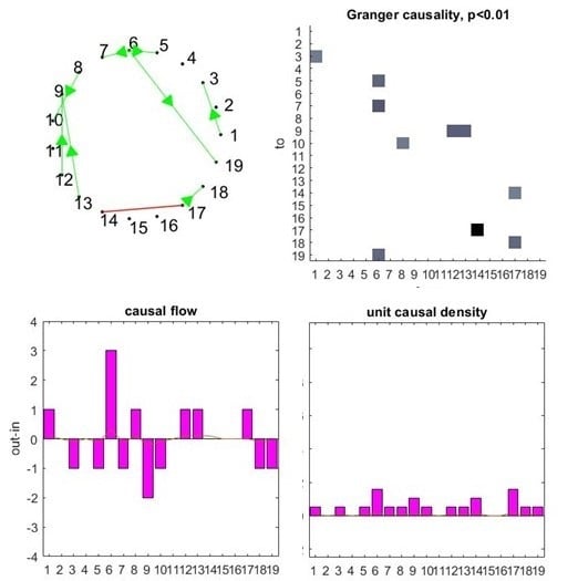
In case study A (model A), nodes 1, 5, 7, 11, 12, and 16 were identified as causal sources (positive bars in the causal flow bar-chart), while nodes 3, 6, 8, 9, 17, and 18 as causal sinks (negative bars) as can be seen in Figure 4.

In general, we observed that node 5 (Italy’s total load forecasted) was the most active variable (strongest driver), while node 8 (DA-Greece) was the most passive (biggest sink).

A connection was observed between nodes 1 and 3 (Italy’s solar forecasted generation and Greece’s solar forecasted generation, respectively) which is fairly explained due to the similar weather conditions of the two countries (diurnal effects).

Italy’s load forecasting (node 5) seems to be strongly correlated with the first differences (changes) in Greece’s and Bulgaria’s load forecasting (nodes 6 and 18, respectively) which is explained mostly due to the similar weather conditions as well.

Furthermore, we observed that DA Italy (node 7) affected the commercial schedule from Italy to Greece (node 9), since the Italian market was highly volatile and liquid, so it faced large excursions (spikes) in its wholesale electricity prices which, in turn, affected the power exchanged between the two countries.

Regarding DA Greece (node 8), which as mentioned was the most passive variable in the specific model, we observed that it was moderately correlated and affected by transfer capacity from Greece to Italy (node 11) and from Italy to Greece (node 12) which as shown in Table 8 were significantly highly correlated (0.998). A rational explanation seems that when the Greece–Italy interconnection was operational, NTC (500MW) comprised a significant value relative to the total demand in Greece. Consequently, DA Greece was highly affected whether Greece–Italy interconnection was operational or not.

A strong bi-directional relation was observed between solar generation in Bulgaria (node 13) and commercial schedules from Bulgaria to Greece which is also explained by the fact that Greece is a major importer from Bulgaria, since the latter has one of the lowest market clearing prices in EU driven by the low marginal costs of its nuclear plants and the low demand needs. So, it is rational to assume that a change in the solar generation of Bulgaria represents an excessive energy production which normally is exported by Bulgarian companies, taking into account that domestic demand for energy is covered by the conventional plants.

Finally, no relation was illustrated between the commercial schedule of Bulgaria and Greece (nodes 16 and 17) and DA prices in Bulgaria (node 15) which firstly seems rather strange. A possible explanation could be the wide margin between DA prices in Greece (higher prices) and Bulgaria. This fact leads electricity traders to commit to long-term contracts exporting energy from Bulgaria to Greece, as there is no commercial risk in that.

7.2. Study B: Cross-Border Trading between Greece and Italy

In case study B (model B), nodes 1, 2, 5, 7, and 11 were identified as casual sources (positive bars in the casual flow bar-chart), while nodes 3, 8, 9, and 10 as casual sinks (negative bars) as can be seen in Figure 5.

In general, we observed that node 2 (wind generation in South Italy) was the strongest driver of the specific network with nodes 8 and 11 (DA Greece and commercial schedules from Greece to Italy, respectively) being the most remarkable sinks. This reflection may hide a relation of active and passive roles in the specific interconnection.

The solar forecasted generation, in South Italy (node 1), was strongly correlated to the Greek forecasted solar generation (node 3). A moderate correlation was also observed between South Italy’s and Greece’s wind generation (nodes 2 and 4). This seems reasonable, taking in consideration the geographical locations and the meteorological conditions of the two regions, South Italy and Greece, having a very similar climate, and it is something we observed from the correlation coefficient in Table 8. However, as mentioned earlier, in the case of wind and solar generation there was no point to discuss the Granger causality, since they are highly stochastic time series. The forecasted South Italy wind generation (node 2) also Granger causes strongly the commercial schedule from Greece to Italy (node 10).

We observed that node 7 (the change in DA price in South Italy), Granger causes nodes 9 (commercial schedule IT-GR) and 10 (commercial schedule GR–IT). But node 7 was influenced or Granger caused by node 5 (Italy’s total load forecast). Also, node 5 had a bi-directional connection with node 6 (Greek total load forecast). This was something expected, since when the wholesale price in Italy was high, traders tried to buy cheap electricity for neighboring interconnected countries, hence the commercial schedules were directly affected. So, load forecasts in both countries Granger cause the DA price in South Italy (which means that the error in forecasting Italy’s load were minimized when considering Greek load forecasts) which, in turn, Granger causes the total commercial schedules between IT–GR and vice versa. This is a very interesting result, indicating that the spot price in South Italy drives the commercial programs in the cross-border trading of both countries.

Node 4 (Greek forecast wind generation) Granger causes node 8 the changes in DA Greek price, as expected (wind generation reduces, in general, Spot prices). The changes in the DA Greek price were driven (Granger caused) by node 11 (the transfer capacity from Greece to Italy) which had a bi-directional connection to the node 12 (transfer capacity from Italy to Greece).

Regarding the casual density of variables under consideration, nodes 5 (Italian forecast load), 7 (changes in DA-price of South Italy) and 11 (transfer capacity from Greece to Italy) showcase the largest values, reflecting their total amount of casual interactivity, which is also a form of dynamical complexity in the network. These three variables were globally coordinated in their activity, within the system produced by model B. This means that they are useful in predicting each other’s activity, as we have seen, but also useful in predicting other variables with different power.

The South Italian forecasted wind generation is the largest casual source, i.e., the variable (node) that exerts the strongest casual influence on the system as a whole, since Granger causes variables 10 and is strongly correlated to 4 (total commercial schedule GR–IT and Greek forecasted wind generation).

8. Conclusions

In the current study, we tried to identify and explain any causalities among energy fundamentals between Greece, Italy, and Bulgaria, using Granger causality theory. Causal connectivity implies a connection that lies on the enhancement of forecasting between two time series. That being said, and according to our knowledge, the lack of similar research on non-market coupled countries makes the current work unique and the outcomes that arise should be taken under consideration especially in the era of the implementation of the ETM.

We designed two models of which the one was reliable (highly consistent) enough to be analyzed. The model that was presented is the one that examines the interconnection between Greece and Italy. The authors could not design a reliable model for the Greece–Bulgaria interconnection. That might be due to the lack of data for the Bulgarian DA price (D21) which forced us to use half of the available data for the rest of the time series as well (in order to have the same number of observations) when examining the specific interconnection.

The results show that there were some causal connections among some of the electricity trading fundamentals which indicate that in order to facilitate the forecasting and minimize errors, we need to include them in the same model. There were also some weaknesses revealed which bring to the surface the need for market coupling among those countries.

It seems that the Italian market has a more active role in the specific interconnection followed by Greece. This could be explained by the fact that Italy is already part of the Central Western European (CWE) region which includes 19 market coupled countries, while Greece is not coupled yet with any of the interconnected countries and thus not so volatile and liquid like the Italian one

The lack of designing a reliable model that explains the causalities between Greece and Bulgaria offers opportunities for further research. Also, it would be interesting to see how the imminent market coupling between Greece and Italy will affect the relations described above.