Modelling the Coevolution of the Fuel Ethanol Industry, Technology System, and Market System in China: A History-Friendly Model


1
International Business School, Shaanxi Normal University, Xi’an 710119, China
2
School of Public Administration, Zhongnan University of Economics and Law, Wuhan 430073, China
3
School of Economics and Finance, Xi’an Jiaotong University, Xi’an 710061, China
*
Author to whom correspondence should be addressed.
Energies 2020, 13(5), 1034; https://doi.org/10.3390/en13051034
Submission received: 14 October 2019
/
Revised: 17 January 2020
/
Accepted: 24 February 2020
/
Published: 26 February 2020
(This article belongs to the Special Issue Challenges and Opportunities for the Renewable Energy Economy)
Abstract
:The interaction among the fuel ethanol industry, the technology system, and the market system has a substantial effect on the growth of the fuel ethanol industry which plays a key role in the formation of a sustainable energy system in China. However, we know little about the relationships among them and it is difficult to explore the nexus using econometric method due to the lack of statistics on China’s fuel ethanol industry. This paper develops a history-friendly coevolutionary model to describe the relationships among the fuel ethanol industry, the technology system, and the market system in China. Based on the coevolutionary model, we further assess the impacts of entry regulations, production subsidies, R&D subsidies, and ethanol mandates on the growth of the fuel ethanol industry in China using a simulation method. The results of historical replication runs show that the model can appropriately reflect the multidirectional causalities between the fuel ethanol industry, the technology system, and the market system. We also found that entry regulation is conducive to weakening the negative economic impacts induced by the growth of the grain-based fuel ethanol industry without affecting the long-term total output of the industry; production subsidies to traditional technology firms are helpful for the expansion of the fuel ethanol industry, but they also impede technology transfer in the industry; only when firms inside the industry are not in the red can R&D subsidies promote technological progress and then further accelerate the growth of the fuel ethanol industry; the ethanol mandate has a significant impact on industrial expansion only when a production subsidy policy is implemented simultaneously. Our findings suggest that more attention could be paid to consider the cumulative effects caused by coevolutionary mechanisms when policymakers assess the effects of exogenous policies on the growth of the fuel ethanol industry. More attention also could be paid to the conditions under which these policies can work effectively.
1. Introduction
Fuel ethanol helps to reduce harmful emissions from vehicles, contributing to the fight against climate change and the pursuit of clean mobility [1]. Moreover, as a kind of renewable energy made from sustainable biomass materials, fuel ethanol is an ideal substitute for the non-renewable fossil fuels [2]. Thus, fuel ethanol is expected to play a key role in the formation of a sustainable energy system. China is the largest consumer of fossil fuels and attaches great importance of the development of the fuel ethanol industry. In 2018, the fuel ethanol production capacity in China reached 3.22 million tons. China has become the third-largest fuel ethanol consuming and producing country, following Brazil and the United States [3]. However, China accounted for just over 3% of global production in 2018. The development of the fuel ethanol industry in China still faces many challenges (e.g., technical uncertainty, demand uncertainty, and feedstock uncertainty) [4,5,6]. The Chinese government announced a new nationwide ethanol mandate that will expand the mandatory use of E10 fuel (gasoline containing 10% ethanol) from 11 trial provinces to the entire country by 2020. If China were to meet the national mandate of E10, it would require an extra 12 million tons of fuel ethanol production capacity, which is about four times that of its current production capacity. Therefore, exploring the nexus among the fuel ethanol industry, the uncertain technology system, and the uncertain market demand will be conducive to clarifying the growth mechanisms of the fuel ethanol industry and then improving public policy to accelerate the growth of the fuel ethanol industry in China.
Many scholars have already analyzed the different factors that affect the development of the fuel ethanol industry. These factors mainly include technology change [7,8,9,10], market demand [11,12,13], feedstocks [8,14,15], renewable energy infrastructures [16,17], energy policies [18,19,20,21], and economic, social, and environmental impacts [22,23,24,25]. These works mainly used case studies [8,10], econometric methods [9,11,12,19], and simulation methods [7,13]. Although the existing literature provides important information on the relationships between the fuel ethanol industry growth and its drivers, there are still some limitations. Firstly, most studies do not consider the adverse impacts of the fuel ethanol industry on its drivers and the interrelationships among the driving factors. The ignorance of the above interactions may lead to a misunderstanding of the growth mechanisms of the fuel ethanol industry [26]. Secondly, the fuel ethanol industry is an emerging industry in China. Therefore, the econometric methods used in the existing studies could not be applied to analyze the development of the fuel ethanol industry in China due to the lack of statistical data. Lastly, although simulation is an ideal method to quantitatively analyze the development of emerging industries, such as the fuel ethanol industry, this method is often questioned because of the subjectivity of its parameter settings [27].
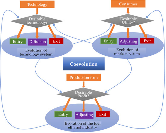
In addressing these limitations, this paper employs a history-friendly evolutionary model to explore the interactions among the fuel ethanol industry and its driving factors and analyze the impacts of different policies on the evolution of the fuel ethanol industry in China. The contributions of our work are reflected in three aspects. First, we argue that there are multidirectional causalities among the fuel ethanol industry, the technology system, and the market system. Therefore, we applied a coevolutionary framework to model the above relationships. Under this framework, each party exerts selective pressures on the others, thereby affecting each other’s evolution [28]. Second, we developed a history-friendly model to depict the above coevolutionary relationships related to the fuel ethanol industry in China. The parameters of the history-friendly model are set based on the historical evolutionary characteristics of the industry but not on historical statistics. Therefore, this method can be used to analyze the growth of the fuel ethanol industry, which lacks historical statistics in China. At last, we further analyzed the impacts of entry regulation, production subsidy, R&D subsidy, and ethanol mandate policy on the evolution of the fuel ethanol industry in China.
The rest of the paper is structured as follows. Section 2 reviews the driving factors that affect the growth of the fuel ethanol industry. Section 3 features a history-friendly model based on the coevolutionary framework, which describes the interactions among the fuel ethanol industry, the technology system, and the market system. In Section 4, we first run the baseline simulation to select the values of the parameters that can reflect the historical characteristics of the fuel ethanol industry and then use this model to further analyze the impacts of several typical fuel ethanol industry policies, while Section 5 contains concluding remarks and policy implications.
2. Literature Review
2.1. The Effects of Technology Change on the Evolution of the Fuel Ethanol Industry
One of the most important factors limiting the scale of the fuel ethanol industry in the United States is technological progress. Fuel ethanol could account for about 10% of total energy consumption if there is no major technological advance, but if technological progress is significant, then this proportion could rise to 20%. This proportion could further rise to 25% if the major usage of the land could be partly converted to planting energy crops [7]. The success of the fuel ethanol industry was not only due to resource advantages but also due to the advantage of technological progress [8]. In addition, the effect of technological progress on the production of fuel ethanol is adjusted by mandatory consumption policies [9].
There is no doubt that technological change has vital impacts on industry evolution. However, the origin of the fuel ethanol industry’s technological progress remains controversial. One of the hypotheses is that technological advantage is derived from the accumulation of knowledge, which is one of the “learning by doing” types [29]. Another opinion is that technological progress is driven by the new energy automobile industry, especially the development of flexible fuel vehicles that began in 2003 [30,31]. In addition, agricultural output is believed to be the main source of the fuel ethanol industry, so the progress of agricultural technology has had an important impact on the development of the fuel ethanol industry [32]. Different actors (e.g., ethanol producers, public and private research institutions, and government institutions) in the industrial chain could also affect technological progress [7]. Some scholars found that more attention should be paid to scientific progress, especially the impact of scientific progress on fuel ethanol technology in recent years [33].
The relationship between the progress of fuel ethanol technology and public policy is very close. However, the focus of the scientific community is different than the focus of the government. The scientific community is concerned about environmental protection and technology, while the government is concerned more about geopolitics. This difference reveals that either the scientific community needs to pay more attention to the knowledge demands of policymakers or that policymakers need to focus more on scientific and technological knowledge [10].
2.2. The Effects of Renewable Energy Policy on the Evolution of the Fuel Ethanol Industry
The development of new technologies in the fuel ethanol industry still faces various barriers [34]. In many countries such as the United States [35], governments have adopted a wide range of policies to support the development of their fuel ethanol industries, especially, to spur the new technologies. These policies (e.g., subsidies, tax cuts, mandatory consumption, and tariff protections) have had important impacts on the development of the fuel ethanol industry. If the government’s subsidy policy is properly designed, it can effectively compensate for the risk difference caused by land quality difference, and further, promote the greater use of marginal land with poor quality to produce energy crops [36]. R&D support policies play an important role in the technological progress of the fuel ethanol industry, and the quantity of public R&D funds directly affects the progress of fuel ethanol technology [7].
Some scholars have investigated the impact of various renewable energy policies on industry evolution. A vertically integrated market model, including fuel ethanol, by-products, and corn, was used to analyze the social impact of the fuel ethanol industry’s subsidy policies, and the results showed that subsidy policies may not lead to positive social benefits [18]. It is also found that the tariff protection and tax-cut policies of biofuels in the United States may lead to the loss of total social welfare [37].
Other scholars analyzed the distortion effect of fuel ethanol policy from the perspective of international trade. If the U.S. government were to cancel tariff protection and reduce the scope of tax cuts, ethanol imports would increase 130%, while domestic ethanol production would fall 9% [11]. The current biofuel trade protection policy in the United States not only reduces the industrial competitive advantage of corn-based ethanol but also increases dynamic learning costs, which will also reduce the international competitiveness of the future cellulosic ethanol industry [38]. No matter how high the carbon tax rate is, a single carbon tax policy without additional subsidies will not promote the evolution of the fuel ethanol industry [19].
Although many studies have noted the distortion effects of fuel ethanol policies, other scholars maintain that subsidies can help to overcome market failure [20]. Gehlhar et al. (2010) evaluated the long-term economic impact of fuel ethanol subsidies in the United States and concluded that the development of the fuel ethanol industry is conducive to lowering the dependence on oil imports, thereby contributing to the development of the overall economy. Further, the overall benefits induced by the subsidy were greater than the welfare losses [21].
However, due to the characteristics of the emerging industry, the future direction of the fuel ethanol industry policy is highly uncertain, which increases the uncertainty of the development of the fuel ethanol industry [39]. The development of the fuel ethanol industry involves issues of food security, energy security, and environmental protection. Therefore, in the process of formulating supporting policies for the fuel ethanol industry, attention should be paid to the integration of these policies [32,40].
2.3. The Effects of Market Factors on the Evolution of the Fuel Ethanol Industry
Since oil and biofuels are substitutes, and crops like corn and sugar cane are the main feedstocks of biofuels, the price of oil, corn, and sugar cane will have an important impact on the evolution of the biofuel industry. An empirical study showed that an increase in oil prices will lead to an increase of biofuel production, while the increase of corn and sugarcane price will lead to a decrease of fuel ethanol production [11]. Government subsidies for the fuel ethanol industry and biodiesel industry should be increased because uncertainty in oil prices and crop yields would affect the evolution of the fuel ethanol industry [12]. It is also found that a 30% drop in oil price would lead to a significant drop in fuel ethanol demand, and, at the same time, fuel ethanol prices would also drop significantly [13].
The cost of feedstocks was found to be the main influencing factor affecting the short-term evolution of the fuel ethanol industry. Therefore, the future R&D of the fuel ethanol industry should focus on the low cost of decomposition from lignocellulose sugar and the comprehensive utilization of lignocellulose [14]. It is also found that an insufficient understanding of feedstock cost is the main reason for the slow progress in the commercial utilization of fuel ethanol in Africa [5].
The above literature sheds important light on the relationships between the fuel ethanol industry and its driving factors. However, the ignorance of the industry’s multidirectional relationships may lead to an inaccurate assessment of the relationship between the fuel ethanol industry and its drivers. Therefore, in order to understand the growth mechanism of the fuel ethanol industry in China, this paper will analyze the relationships among the fuel ethanol industry, the technology system, and the market system using a history-friendly coevolutionary model. This paper will further assess the impacts of several policies (i.e., entry regulation, production subsidy, R&D subsidy, and ethanol mandates) on the growth of the fuel ethanol industry.
3. The Model
3.1. The History-Friendly Model
As an emerging industry in China, there are limited statistics of the fuel ethanol industry. Therefore, it is difficult to analyze the mechanisms and factors affecting the fuel ethanol industry using a statistical model. In order to explore the coevolutionary relationships between the fuel ethanol industry, the technology system, and the market system, this paper employs a history-friendly evolutionary model which has been applied to many industries, including computers, DRAM chips, pharmaceuticals, semiconductors, synthetic dyes, and mobile phones and memory chips [41,42,43,44,45,46]. Scholars studying industrial dynamics generally rely quite heavily on the appreciative theory which is a body of verbal arguments representing causal explanations of observed patterns of economic phenomena [47,48]. Although the appreciative theory is an appropriate tool to characterize the main mechanisms at work, it is difficult to verify the logical consistency of the theory due to its complexity and the lack of precision of the verbal language [47]. The history-friendly model is a formal model of the appreciative theory and can overcome the above limitations of the appreciative theory [41]. It aims to analyze, in a more formal form, the influential factors and their influencing mechanisms in industry evolution, technological progress, and institutional change that have been confirmed by appreciative theory [41,49].
The construction of the history-friendly model consists of three important steps [47]. The first step is the selection of the stylized facts deserving attention from theoretical perspectives. These stylized facts mainly refer to the history and evolution of the fuel ethanol industry such as specific institutions, technological change, and market characteristics. Second, there is the choice of how to represent the selected phenomena. In this respect, the history-friendly model adopts the same basic representations used in evolutionary models. All reported models are built around four main blocks: firm behavior, technological change, market demand, and industry dynamics [50,51]. The creation, entry, exit, and technological change of the business firms affect the performance of the industry and further impact industry evolution. The third step is the manipulation and implementation of the model designed in the second step.
The history-friendly model is a type of agent-based simulation model dealing with the complexity of the economic system [52]. A typical history-friendly model has many variables and parameters. Under a wide range of parameter settings, some of the parameter settings will lead to the replication of the industry history being modelled. Importantly, “replication” here mainly refers to qualitative reproduction, not quantitative reproduction [53]. Once the model is built, there is room for wider applications such as policy analysis. The history-friendly nature is threefold. Firstly, in the process of model construction, stylized facts in industrial development are fully considered, and the relationship between variables is constructed on this basis. Secondly, the initial values of variables in the model are set based on the true values of industrial history. Thirdly, the selection of the parameters’ values can qualitatively reproduce the stylized facts in industrial history.
There are two compelling reasons for using a history-friendly model in this paper. First, a history-friendly model helps us better explore the causal mechanisms in the evolution of the fuel ethanol industry. As a formal model, all the logic that drives model outcomes is explicitly represented in a history-friendly model [27]. In addition, the mechanisms built into the model are transparent which means that if the model does not work as expected, the analyst can adjust the settings of the model until the model is able to qualitatively capture the stylized facts in the appreciative theory [54]. Developing and working through a history-friendly model could bring to mind mechanisms, factors, and constraints of the industry evolution [41]. Therefore, compared with the appreciative theory, the history-friendly model is conducive to analyzing the causal mechanism of the fuel ethanol industry. Second, the model setting of the history-friendly model is transparent rather than arbitrary, so, it serves as a good starting point for further policy analysis. Comparing the influence of different systems and policy arrangements on industry evolution can provide a deep understanding of the influence mechanism of the above factors and provide a basis for further policy selection and institutional arrangement [41,55].
3.2. The Model Specification
The basic model is presented in this section. Given the complexity of the history-friendly model, it is difficult to lay out all the details of all the equations without confusing the reader and obscuring the basic logic of the model [41]. Therefore, we have tried to present only the equations which can reflect the stylized facts of the fuel ethanol industry and put other related equations in the Appendix A. Just like most of the other history-friendly models [50,51], our model is also built around four main building blocks: firm, technology progress, market demand, and industrial dynamics. In selecting the stylized facts to investigate, we considered their relevance on the selection of the variables and the relationships among these variables, which affect the model specification [47]. These stylized facts are put at the beginning of each block. In addition, given that our model involves many subjects which are further divided into different types, we use a lot of superscripts to minimize the number of variables used in the model. The variables with superscripts b and f represent the variables associated with the properties of fuel ethanol and fossil fuels, respectively. The variables with superscripts tf, nf, and rd represent the variables associated with the properties of traditional technology firms, new technology firms, and R&D firms, respectively. The variables with superscripts m and t represent the variables associated with the properties of materials and traditional materials, respectively.
3.2.1. Firm
(1) R&D investment of the firm
As a typical emerging industry, the fuel ethanol industry is still faced with the urgent need for continuous improvement of its related technologies. Therefore, one of the stylized facts is that almost all firms in the fuel ethanol industry have research and development (R&D) investments. We assume that the firm’s R&D investment consists of two parts. The first part is the fixed amount of R&D investment. Whether the company is profitable or not, it will invest in R&D. The second part is that when the firm has a positive profit, a fixed proportion of profit will be invested in R&D. Thus, R&D investment can be expressed as:
where rd denotes the fixed amount of R&D investment; σ denotes the fixed proportion of profit invested in R&D, and πit denotes firm’s profit which is defined by Equation (A7) in the Appendix A.
(2) Entry of firms
We assume that a firm’s entry decision is influenced by the industry’s profit to cost ratio. Let , where and are positive constants, and is given a distribution function , s = 1,2...,l; then, the number of latecomers in each period can be expressed by the following equation:
where .
In Equation (2), if is set; then, , which represents when the incumbent firm loses money, and no new firms enter this industry. That is to say, indicates that the firm is completely rational. If is set, even if the incumbent firms have losses, there will still be latecomers. In other words, this model can satisfy the theoretical hypothesis of rationality or incomplete rationality by making different assumptions.
This study assumes that the initial size and technical efficiency of the latecomers are equal to the average level of the whole industry.
(3) Adjustment rules of the firm
During each period, the firm can determine the optimal output, , and the corresponding demand of feedstock, , according to the feedstock price and product price. Due to the matching relationship between the feedstock input and fixed assets, the required asset size should be . If the firm’s own asset scale is smaller than , then the firm’s asset scale expands to , and the corresponding firm’s capacity utilization ratio is . Otherwise, if the firm’s own asset scale is larger than , the firm’s asset scale remains unchanged, that is , and the capacity utilization rate is .
(4) Exit rules of the firm
We assume that when the firm has losses for several consecutive periods, the firm will withdraw production.
3.2.2. Technology Progress
(1) Progress and Diffusion of Traditional Technology
There are four stylized facts of the technological progress in China’s fuel ethanol industry. First, traditional production technology is relatively mature, so technological progress is mostly reflected in the continuous improvement of the original technology. However, there are a few major technological innovations. In other words, with an increase in the degree of technological progress, the occurrence probability of technological progress rapidly decreases. Second, R&D investment will improve the probability of technological progress. Third, the higher the original level of technology, the lower the probability of major innovation. Finally, due to technology diffusion, the technological progress of a specific firm is positively correlated with the most advanced technology level in the industry.
In this study, it is assumed that there is the highest level of technical efficiency boundary, denoted as . Let be the change of the firm’s technical level; then, the technology change will not exceed the difference between the firm’s technical level and the highest level . Therefore, the firm’s technology change is
where is the random variable of the interval [0,1], in order to reflect the first stylized fact of technological progress, that is, the larger the degree of technological progress, the smaller the occurrence probability.
We construct variables and assume Poisson distribution with parameters and . Then, there is
where is the mean value of the random variable . The larger the value, the higher the probability that the technical efficiency will be greatly improved. The technology R&D investment, , is positively correlated with , which reflects the second stylized fact of the above mentioned technological progress. The gap between the firm’s technical level and the highest technical level, , is positively related to , which reflects the third stylized fact. reflects the gap between the technological level of the firm and the highest technological level in the industry. This value is positively correlated with , which reflects the fourth stylized fact of technological progress—the diffusion of advanced technologies in the industry. ,,, and are nonnegative constants.
Finally, when the technical level of the firm reaches its highest boundary value, the firm will stop its R&D investment.
(2) Entry, Progress, and Exit of New Technology
Due to the insufficient supply of feedstock, another stylized fact of China’s fuel ethanol firms is that firms need to constantly explore new feedstock and corresponding production technologies. Due to the diversity of fuel ethanol feedstock, the corresponding production technology also shows diverse characteristics. The adoption, progress, diffusion, and withdrawal of different production technologies lead to the change of technological diversity in the industrial technology system, thus promoting the evolution of the technology system.
The entry rules of new technology: This research focuses on the evolution of production technology, which is closely related to industry evolution. Therefore, we use the innovative activities of an R&D firm to describe the evolution of new technology. An R&D firm is a corporation whose output is new technology while the R&D expenditure is its input. We assume that when the industry profit of using traditional technology is negative, new R&D firms start to enter the industry, and the number of entries is random. Among them, the number of R&D firms created by the incumbent firm and the number of completely new R&D firms is both randomly selected from 0,1......, . Upon entry, all newly created R&D firms are faced with the same initial technical efficiency level, and if an R&D firm already exists in the technology system, the newly created R&D firms will search for the maximum technical efficiency in the existing R&D firms as its initial technical efficiency. The change in the technical efficiency of R&D firms is expressed as follows:
In this model, the entry of R&D firms is used to reflect the evolution characteristics of new technologies in the industry. There are two forms of entry for R&D firms: one type of firm is newly created by incumbent firms, and the other is a random start-up. The R&D output of these two kinds of R&D firms is mainly determined by the efficiency of technical output and the amount of R&D input. If the newly established R&D firms have the same total amount of R&D capital, , and take a fixed proportion of the R&D capital as the R&D investment in each period, the differences between the two kinds of newly established R&D firms include two elements. First, since newly established R&D firms are usually more flexible than incumbent firms, and the flexibility of the system is more conducive to the formation of new technologies, newly established firms will have higher R&D productivity than incumbent firms, which is mainly reflected in the difference between the two types of firms in terms of value [43]. Second, as mentioned above, new technology may replace old technology, which will lead to a sunk cost loss for the incumbent firm. Therefore, the incumbent firm will reduce the proportion of R&D investment, which is negatively correlated with the residual fixed assets of the original firm. Its R&D investment is
and the newly established firms take a fixed amount as the R&D investment:
where is a constant. Equations (6) and (7) mean that before the depreciation of fixed assets is completed, the R&D input of the incumbent firm will be less than the R&D input of the new firm.
New technology adoption rules: Firms will only adopt new technology when the average cost of production using that new technology is lower than the average level of traditional technology. This means that, before a firm is able to enter the market, it must go through a long R&D period. During this period, it is difficult for the firm to generate profits and maintain survival. Therefore, in the start-up stage of the new R&D firm, that firm must rely on external capital which is reflected as the initial capital stock of the new R&D firm in this model.
Rules for R&D firms to withdraw from R&D activities: When the initial capital stock is all used for R&D expenditures, and the production costs of new technology still do not reach the average levels of those of traditional technology, the R&D firms will choose to withdraw, which means the withdrawal of new technology.
3.2.3. Market Demand
There are three stylized facts in the production market of the fuel ethanol industry in China. First, fuel ethanol is a typical emerging product whose market demand is gradually forming and expanding or shrinking. Second, there is a competition between fuel ethanol and liquid fossil fuels. The market demand for fuel ethanol comes from the substitution of the market demand for fossil fuels. Third, the government can intervene in the fuel ethanol market through legal or administrative measurements.
In the production market, fuel ethanol is directly incorporated into the formal gasoline sales network, which is an oligopoly market. This means that the price of fuel ethanol will be consistent with gasoline prices, which are decided by the supplier as follows:
where denotes the price of fuel ethanol, denotes the price of gasoline, and denotes the markup percentage.
In pilot provinces, the demand for fuel ethanol will reach a larger scale in the short term after the implementation of the pilot because the pilot consumers can only purchase E10 gasoline. On the other hand, the output of fuel ethanol is relatively smaller in the early stages of the fuel ethanol industry. This means that market demand is horizontal before reaching a specific value but becomes vertical after reaching a specific value. Therefore, Equation (8) can be regarded as the demand function of the fuel ethanol market.
Then, we need to consider the entry, adjustment, or exit of the consumer. As mentioned above, the evolution of the fuel ethanol market is reflected in the entry of potential consumers and the adjustment of consumption by incumbent consumers or the exit from the market.
Consumer Entry Rules: As the consumption of E10 is mandatory, new consumers of fuel ethanol will enter into the market with the expansion of pilot areas.
Consumer Adjustment Rules: When the price of fuel ethanol remains constant, the changes in demand only affected by the changes in consumer’s fuel spending. Therefore, consumers will increase or decrease their demand for fuel ethanol based on changes in total fuel spending. The adjustment to fuel ethanol purchases for specific consumers is
where denotes the percent change in fuel ethanol demand for consumer j in period t; denotes the percent change in consumer j’s income in period t.
Consumer Exit Rules: Consumers who are not satisfied with the consumption of fuel ethanol will choose to exit the market.
3.2.4. Industrial Dynamics
(1) Entry of Production Firms
Production firms in the fuel ethanol industry are divided into two types: one is the traditional technology firm which mainly uses traditional production technology and the other is the new technology firm which mainly uses new production technology. Let denote the number of traditional technology firms entering in period t. According to the previous section, it is related to and , which indicate the cost to revenue ratio of traditional technology firms and the number of firms in the industry of the last period respectively, as well as the random distribution function . In addition, in the fuel ethanol industry, the entry of traditional technology firms is also restricted by the shortage of feedstocks. Then, we can describe the number of traditional technology firms as follows:
where represents the demand for traditional feedstocks in the last period.
There are two kinds of new technology firms entering in period t in the fuel ethanol industry: one is transformed from R&D firms, which is denoted by ; the other includes newly established firms that use new technology, denoted by the parameters’ values . According to the above definition, is related to the number of R&D firms in the last period, , its production costs in the last period, , and the highest production cost in the last period, , which can be shown as:
is related to the cost of new technology firms in the last period, , to the revenue rate, the number of new technology firms in the industry, , and random distribution function, , so:
(2) Exit of Firms
According to the above rules, when a firm loses money in a continuous k-period, it will exit from production. If the number of withdrawing traditional technology firms in period t is denoted by , and the number of withdrawing new technology firms in period t is denoted by , then there are
(3) Change in the Number of Firms in Production
Then, the number of traditional technology firms in period t is
The number of new technology firms in period t is
The total number of firms involved in the production in the industry at period t is
According to Equations (15) and (16), the entry or exit of firms in an industry is influenced not only by the industrial system itself but also by the evolution of the market system and technology system.
4. Results and Discussion
4.1. History Replicating Runs
4.1.1. Baseline Scenario
The aim of the history replicating runs is to find a set of parameters values, based on which the simulation results can reflect the historical stylized facts of the fuel ethanol industry in China [56]. This kind of replicated history is also called the baseline scenario which could be used as a starting point for further policy assessment [57]. Therefore, it is important to select the historical stylized facts that the simulation results intend to capture. Given that the ultimate purpose of our paper is to understand how the fuel ethanol industry has grown, we mainly focused on the following stylized facts about the number of firms and the output of the fuel ethanol industry in China, which are derived from a detailed analysis of the industrial history and from the existing appreciative literature on the fuel ethanol industry in China [58,59].
- (1).
- Once established, traditional technology firms would not withdraw even if they lost money, because the government subsidized loss-making firms to foster the growth of new energy industry.
- (2).
- There is a ceiling of the number of the traditional technology firms because the available raw materials (i.e., expired corn and wheat) used by these firms are limited.
- (3).
- All R&D firms established by the incumbent traditional technology firms failed to transform into new technology firms.
- (4).
- All new technology firms are derived from newly established firms with new production technology rather than the firms transforming from R&D firms.
- (5).
- The number of incumbent firms also has a ceiling because the maximum market capacity is fixed. When the aggregated output of the fuel ethanol beyond the maximum market capacity, there would be no new firms entering the industry.
- (6).
- The total output increased faster before the number of traditional firms reached the ceiling because the increasement of the total output is mainly caused by the entry of traditional technology firms.
- (7).
- When the number of traditional technology firms reaches the ceiling, the growth rate of their total output will decrease significantly, because the increasement of the total output is mainly caused by the relatively small expansion of the incumbent firms.
- (8).
- When the new technology firms start entering the industry, the total output will increase faster again until there is no entry of the new technology firms.
In order to find the set of parameters values which can ‘reproduce’ the above-mentioned stylized facts, the following steps used in most of the relevant literature were employed in this paper [46,51,60,61]. Firstly, we set the initial values of the variables in the system based on the historical data of the fuel ethanol industry in China. These initial values are shown in Table A1 in Appendix A. Then, we divided the parameters into two groups when setting the values of the parameters. The first group includes the parameters (e.g., the rate of depreciation) which can be set based on the industry history. In these cases, it is possible to fix the parameter to one value. The second group includes other parameters (e.g., the degree of firm rationality) which could not be set to a fixed value for the lack of enough data to estimate its exact value. Thirdly, for the second group of parameters, we did not attempt detailed quantitative matching to historical data, reflecting our ignorance about their ‘true’ values. Alternatively, we chose values randomly in the predetermined ranges of the parameters and then adjusted the values until the simulation results could qualitatively capture the stylized facts. To adjust the values of the parameters more efficiently, we assessed each parameter’s impact on the simulation results, respectively, through keeping all parameters but one constant and then gave preference to adjusting the parameters which had greater impacts. Once the simulation results about the output and the number of firms could qualitatively reflect all the above eight stylized facts, we stopped the adjustment and chose this set of values as the parameters’ values under the baseline scenario. Although ‘qualitatively reflect’ means that there may be many sets of parameters values satisfying the above condition, we did not need to judge which was the best one to reflect these stylized facts because the aim of the history-friendly model was to explore the causal relationships rather than the magnitude of the effects between variables. The final values of parameters are shown in Table A2 in the Appendix A. An additional constraint orienting the choice of parameter values was provided by the time structure of the model, because the definition of what ‘one period’ means in real-time (half a year in this model) is crucial for establishing which actions take place at any one period. The simulation is implemented using Mathematica software package. The results under the baseline scenario are shown in Figure 1, Figure 2, Figure 3 and Figure 4.
Figure 1 shows the change in the number of firms in the fuel ethanol industry under the baseline scenario, which can be divided into four stages. There were only traditional technology firms in the first stage, and the number of firms kept increasing. The second stage starts after the 17th period, during which the number of traditional technology firms was no longer increasing. At the same time, R&D firms with new technology appeared, and their numbers increased gradually. However, after the 22nd period, the number of R&D firms began to decline. On the one hand, some R&D firms transformed into production firms and began to produce fuel ethanol. On the other hand, some R&D firms failed to survive because they did not meet the expected innovation goals. The third stage starts in the 26th period. New technology firms began to produce at this stage, and their number increased gradually due to the establishment of the new technology firms and the transformation of R&D firms to new technology firms. According to the simulation results, all production firms transformed from R&D firms are originated from the newly established R&D firms, while the R&D firms created by traditional technology firms failed to transform into production firms, which is consistent with the evolutionary history of the fuel ethanol industry in China. The fourth stage starts from the 31st period. Due to the limitation of market capacity, the number of new technology firms is no longer increasing, and the number of firms in the market remains stable.
Figure 2 shows the change in the output of the fuel ethanol industry under the baseline scenario, which is divided into four stages. In the first stage, the total output of the industry increased continuously. The total output curve coincides with the output of traditional technology firms since there are only traditional technology firms in the industry. The second stage starts from the 17th period when the number of traditional technology firms was not increasing. Although the total output was still increasing, the growth rate of the total output decreased significantly. The increase in output mainly comes from the increase in the output of incumbent firms. The 25th period indicates the third stage: with the entry of new technology firms, the total output began to increase rapidly until the 31st phase. Due to the limitation of market capacity in this period, the number of new technology firms did not increase. The output growth of new technology firms significantly dropped again and then entered the fourth stage. The total output growth is relatively low since there is no entry of new firms. The increase of output in this stage mainly depends on the expansion of the production scale of existing firms.
Figure 3 shows the change of the average technical efficiency of traditional technology firms, R&D firms, and new technology firms under the baseline scenario. The average technical efficiency of all three kinds of firms is increasing. However, the extent of this increase varies from firm to firm. The average technical efficiency of traditional technology firms changes relatively slowly, while the average technical efficiency of R&D firms improves relatively quickly. The average technical efficiency of new technology firms improves rapidly in the initial stage of production but tends to be flat in later stages. The main reason for the above difference is that the technological progress of R&D firms is significantly faster than that of existing production firms. The average technical efficiency of all R&D firms improves relatively quickly because the technical progress among R&D firms is cumulative, and new R&D firms will absorb the experience of existing R&D firms. In the initial stages of production, new technology firms usually adopt the most advanced technology, which significantly improves the average technical efficiency of the whole industry. When the entry of new technology firms stagnates, the improvement of average technical efficiency only depends on the technological progress of incumbent firms. As a result, the rate of technological progress becomes relatively slow.
Figure 4 describes the technology transformation in the fuel ethanol industry under a baseline scenario. Technology transformation refers to the transformation of the industry from traditional production techniques to new production technology. The proportion of the output of new technology firms to the total output of the industry is used to measure technology transformation. According to Figure 4, the value of the technology transformation has rapidly increased since the 25th period and reached about 32% in the 31st period. However, the growth rate of technology transformation has declined rapidly because new technology firms have closed entry to the industry. This means that technology transformation mainly depends on the continuous entry of new technology firms. When there is no continuous entry of new technology firms, the competitive advantage of traditional technology firms in incumbent firms is comparable to that of new technology firms, so, the market share of traditional technology firms will not significantly decrease.
4.1.2. Robustness Test
Simultaneous simulation of “History Replication” and “History Divergent” for the same industry is a commonly used method to test the robustness of the setting of the parameters’ values [41,44,62]. The characteristics of the biodiesel industry under the baseline scenario are simulated by adjusting the parameters and setting the initial values according to the stylized facts of the biodiesel industry in China. The simulation results are shown in Figure 5 and Figure 6. The characteristics of the biodiesel industry evolution are significantly different from those of the fuel ethanol industry evolution. This means that the simulation results of the coevolutionary model set in Section 3.2 are indeed affected by the parameter settings. Therefore, the setting of the parameters’ values and the initial values under the baseline scenario can be used for further policy analysis.
4.2. Policy Impacts Simulation
4.2.1. The Impacts of Entry Regulation
Entry regulation is one of the most important industry regulation policies. The government often uses this kind of policy to avoid overcapacity or other negative social or economic impacts due to overheating industrial development. Entry regulation has also been used in the management of the fuel ethanol industry. How effective is this policy? Does this policy have any other impacts on the industry’s growth while achieving its policy objectives? These questions are essential for evaluating the performance of regulation policy. To shed some light on the above questions, we analyzed the impacts of entry regulation on the fuel ethanol industry’s evolution using the simulation method. The simulation results are shown in Figure 7, Figure 8 and Figure 9.
In order to prevent the sharp rise in grain prices due to the rapid development of the traditional grain-based fuel ethanol industry, the Chinese government has implemented an entry regulation that restricts the new establishment of grain-based fuel ethanol firms. The results in Figure 7 show that this regulation policy effectively suppresses the demand for traditional feedstock (e.g., corn and wheat). However, an entry regulation has no significant impact on grain price (shown in Figure 8), because the demand for grain as feedstock for the fuel ethanol industry is only a small part of the total grain demand. Figure 9 shows that the growth of the fuel ethanol production decreases in the short term due to entry regulations. However, in the long run, the restraint effect of entry regulation on production will be eliminated due to the creation of new technology firms. Therefore, entry regulation is conducive to restricting the expansion of the grain-based fuel ethanol industry in the short term, while the long-term impact on the fuel ethanol industry is not too large. Moreover, this policy is helpful in promoting new technology and accelerating technology transformation.
4.2.2. The Impacts of Production Subsidy
A production subsidy is one of the most common policies for the government to promote the development of an emerging industry. Whatever the form of the subsidy, the mechanism of the subsidy is to avoid the losses caused by an immature technology and market in the early stages of the industry so that incumbent firms can continue to produce and improve their technology. With the improvement of technology and the market environment, firms will face competition in the market and make normal profits. Figure 10 and Figure 11 show the impacts of a production subsidy on the output and the number of firms in the fuel ethanol industry, respectively.
As shown in Figure 10 and Figure 11, under no production subsidy scenario, firms will continue to enter randomly, and some will withdraw because of losses. Therefore, the industry output and the number of firms will remain at a low level for a long time. However, under the production subsidy scenario, the number of firms entering production will continue to increase, and the output will also continue to rise. The figures also show that the growth rate of the output declined significantly because of the entry regulation on grain-based fuel ethanol firms after the 20th period. Only when new technology firms enter the industry does the output increase significantly again. Therefore, although the simulation results indicate that a subsidy promotes industry growth, this is not a general conclusion. A production subsidy only promotes the growth of subsidized firms and the industries constituted by these firms. When there are different technological routes in the development of the fuel ethanol industry, the implementation of a single subsidy policy may not promote—or even hinder—the development of the industry.
4.2.3. The Impacts of R&D Subsidy
A subsidy for R&D activities helps to accelerate technological progress by increasing R&D investment. Therefore, an R&D subsidy policy is widely used to promote industry growth. In terms of the fuel ethanol industry, there are not only traditional technology firms but also new technology firms and R&D firms in the industry. This section will analyze the differences in the policy effects of R&D subsidy given to different types of firms. To reduce the influences of random factors, the impacts of the R&D subsidy on average technical efficiency industry output were all simulated 10 times. The simulation results are shown in Figure 12, Figure 13, Figure 14 and Figure 15.
The results in Figure 12 and Figure 13 show that the R&D subsidy promotes the technical efficiency of the fuel ethanol industry significantly, regardless of the R&D subsidy for traditional technology firms, R&D firms, or new technology firms. However, in terms of industrial scale, the results in Figure 14 and Figure 15 show that the R&D subsidies have no significant impact on industry output, regardless of the subsidy to traditional technology firms or new technology firms. The reason for this result is that firms in the fuel ethanol industry are all in the red and obtain their production subsidy from the government. Therefore, the improvement of firms’ technical efficiency, which is partly caused by the R&D subsidy, has little influence on the output decisions of firms. This means that when firms are in the red, the influence mechanism of the R&D subsidy to promote a firm’s output will be hindered.
4.2.4. The Impacts of Ethanol Mandate
In order to accelerate the development of the fuel ethanol industry in its early stages, the Chinese government implemented an ethanol mandate policy that required the gasoline sold in pilot cities to contain 10% fuel ethanol. Will this policy help the development of the fuel ethanol industry? To answer this question, we simulated the impacts of the ethanol mandate policy on the output of the fuel ethanol industry. The simulation results are shown in Figure 16.
The result in Figure 16 shows that when there is no production subsidy for losses of firms, the ethanol mandate has no obvious impact on industry output. However, under the subsidy loss scenario, the ethanol mandate will obviously accelerate the development of the fuel ethanol industry. The reason for this phenomenon is that fuel ethanol firms are usually in the red while the industry remains in its embryonic stage. Firms enter the industry randomly and then exit due to continuous losses, so the fuel ethanol industry scale is relatively small. This means that the equilibrium output of the fuel ethanol industry is mainly affected by the number of incumbent firms but not changes in market demand. Therefore, the ethanol mandate has no obvious influence on the output of the fuel ethanol industry, but when firms obtain a loss subsidy, the number of firms will continue to increase, and the industrial output will increase rapidly and reach a larger scale. In this context, the equilibrium output will be mainly affected by market demand. Therefore, an ethanol mandate policy will be helpful to promote the expansion of the fuel ethanol industry.
5. Conclusions and Policy Implications
The interaction among the fuel ethanol industry, the technology system, and the market system has a substantial effect on the growth of the fuel ethanol industry which plays a key role in the formation of a sustainable energy system in China. However, we know little about the relationships among them and it is difficult to explore the nexus using an econometric method due to the lack of statistics on China’s fuel ethanol industry. In order to investigate the coevolutionary relationships between the fuel ethanol industry system, technology system, and market system in China, this paper developed a history-friendly simulation model. The setting of the initial values for the simulation model is based on the historical values of the fuel ethanol industry system, technology system, and market system in China. The parameter values of the model were acquired by adjusting the parameters’ values continuously until the simulation results could reflect the stylized facts of the fuel ethanol industry. According to the baseline model, this paper further assessed the impacts of entry regulation, production subsidy, R&D subsidy, and ethanol mandate on the growth of the fuel ethanol industry. The results show that multidirectional causalities reflected by the coevolutionary model developed in this paper can describe the relationships between the fuel ethanol industry, technology system, and market system appropriately. This means that the evolution of the fuel ethanol industry interacts with the evolution of the technology system and the market system. Meanwhile, the evolution of the technology system also interacts with the evolution of the market system. Entry regulation is conducive to weakening the negative economic impacts (e.g., rising grain prices and grain shortages) of the expansion of the grain-based fuel ethanol industry without affecting the long-term total output of the industry. A production subsidy for traditional technology firms is helpful to the expansion of the fuel ethanol industry. However, this subsidy also impedes technology transfer in the industry. In terms of R&D subsidy policy, only when the firms inside the industry are not in the red can an R&D subsidy promote technological progress and further accelerate the growth of the fuel ethanol industry. The ethanol mandate policy has a significant impact on industrial expansion only when a production subsidy policy is implemented at the same time. This policy can also speed up the improvement of new technology efficiency by advancing the creation of R&D firms and new technology firms.
According to the above conclusions, the policy suggestions are as follows: firstly, an assessment of the effects of an exogenous factor on any one of these three systems must consider the cumulative effects caused by the coevolutionary mechanisms. Secondly, in the context of this uncertain industry’s economic and social impact in China, implementing an entry regulation would be helpful to promote the steady growth of the fuel ethanol industry. Thirdly, when the optimal technology path has not been determined in the Chinese fuel ethanol industry, it will be necessary to implement a production subsidy combined with a new technology promotion policy to avoid technology lock-in. Fourthly, considering that most firms in the fuel ethanol industry in China are still running under a deficit, an R&D subsidy for production firms needs to be implemented along with a production subsidy for unprofitable firms. Lastly, the Chinese government can accelerate the development of the fuel ethanol industry with the help of an ethanol mandate policy. Additionally, the ethanol mandate policy should be implemented together with the production subsidy policy if a firm is running under a deficit.
6. Limitation and Future Research
One limitation of this study is that it does not check the robustness of the simulation results using a statistical approach. It is difficult to estimate the values of the parameters in our model using a statistical method for the lack of enough observations and the complex nonlinearity of the history-friendly model. Alternatively, we employed a process used in most literature about the history-friendly model to determine the values of the parameters in our model. The aim of the process is not the specification of the model parameters as close as possible to their actual values, nor is to explain the quantitative values observed in the historical episode under investigation. Rather, the objective is just to seek a set of parameters’ values which can generate simulation results qualitatively capturing the stylized facts of the industrial history, because the purpose of history-friendly modelling is to explore the causal relationships and the mechanism between variables in the model [44]. This means there may be many sets of parameters’ values that satisfy the requirement. Therefore, after determining a set of parameters’ values for the base case, it is necessary to check the robustness of the simulation results. There are two commonly used approaches to test the robustness in the existing literature [41,47]. One is the inspection of individual runs of the model and the analysis of sensitivity to specific parameter values. The other is the running of a history divergent simulation. These two approaches are also used in this study to check the robustness of the results. However, we suggest there should be a more intense discussion of sensitivity analyses using a statistical method in future research because the above two commonly used approaches could not completely reflect the impacts of stochastic components on the simulation results. Some scholars have already made a bit of progress in this direction. For example, Brenner and Murmann initially developed a process to define the values of the parameters that can be observed with precision [61]. Landini et al. introduced a statistical method which can be used to check the robustness of their results with different variation in the ranges of the parameters [46]. However, both statistical methods have their own drawbacks. The first one turns out not to be immediately comprehensible and could not be completely and clearly described due to the usual limits imposed on the number of words for a paper [50]. The second is still arbitrary in the selection of the variation in the range of parameters. Future research can further improve these two statistical methods and then apply them to the testing of the robustness of the simulation results.
Author Contributions
Conceptualization, C.B. and J.Z.; methodology, C.B. and W.Z.; software, C.B. and Y.W.; formal analysis, C.B. and J.Z.; data curation, W.Z.; writing—original draft preparation, C.B., J.Z., and W.Z; writing—review and editing, C.B.; visualization, C.B. All authors have read and agreed to the published version of the manuscript.
Funding
This research was funded by the fund project of the National Natural Science Foundation of China (Grant No: 71974203), Zhongnan university of economics and law graduate education achievement award cultivation project (Grant No: CGPY201904), interdisciplinary innovation research project (Grant No: 2722019JX002), Zhongnan University of Economics and Law Fundamental Research Funds for the Central Universities (Grant No: 2722020JCT026), the Chinese National Funding of Social Sciences (Grant No: CFA150151), and the Fundamental Research Funds for Shaanxi Normal University (16SZYB34).
Acknowledgments
We thank three anonymous referees for very useful comments.
Conflicts of Interest
The authors declare no conflict of interest.
Appendix A
A1. Modeling the Basic Characteristics of the Firms in the Fuel Ethanol Industry in China
(1) The Production Capacity and Output of the Firm
The production capacity of the firm is related to the fixed capital input of the firm . The variable input of the firm is denoted as
where represents the capacity utilization rate of firm i at time t, and . A value of equal to 0 indicates that the firm stops production. represents the maximum variable input combined with a one-unit fixed input.
We assume that the output of the firm is determined by the input and technical efficiency. The output of the firm is
where denotes the technical efficiency of firm i at time t, and parameter z (0 < z < 1) reflects diminishing marginal productivity.
(2) Production Cost
The total cost of the firm, which consists of the fixed cost and variable cost, is
where represents the depreciation rate; denotes fixed cost; is the price of feedstock; is the input amount of the feedstock; is the variable cost. Considering the relationship between a firm’s input and output described by Equation (A2), Equation (A3) can also be expressed as
The cost per unit of the firm is
The average per-unit cost of the industry is
where represents the number of firms in the industry.
(3) Profit of the Firm
Let be the price of fuel ethanol; then, the firm’s profit is denoted as:
(4) Supply Function
We assume that a specific firm makes production decisions according to the profit maximization principle; then, the supply function of the firm, which is obtained by taking the derivative of the profit equation (Equation (A7)) with respect to output quantity, is
The supply function of the industry, which can be obtained by summing up the supply function of all firms, is
(5) Feedstock demand function
Substitute the relationship between the firm output and the feedstock input of Equation (A2) into Equation (A8); then, the feedstock demand function of the firm can be denoted as
The feedstock demand function of the industry, which can be obtained by summing up the feedstock demand function of all firms, is
(6) Average Size of the Firm and Technical Efficiency in the Industry
Let the firm’s size be denoted by the firm’s fixed input, so the average size of the firm in the industry is
The average technical efficiency of the industry is reflected by the average technical level of all firms in the industry; then, the average technical efficiency of the industry is
The industry’s average profit to cost ratio is
A2. The Initial Values of the Variables in the Coevolutionary Model of the Fuel Ethanol Industry

Table A1.
The initial values of the variables in the coevolutionary model of the fuel ethanol industry (baseline scenario).
Table A1.
The initial values of the variables in the coevolutionary model of the fuel ethanol industry (baseline scenario).
| Initial Values | Description |
|---|---|
| n[[1]]=1 | The total number of firms in the first period. |
| f[[1,1]][[1]]=0 | Types of technology firm: 0 denotes traditional technology firms; 1 denotes new technology firms. |
| f[[1,1]][[2]]=1 | Production status of firms: 0 is no production; 1 is in production. |
| f[[1,1]][[3]]=0.3 | Technical efficiency of firms. |
| f[[1,1]][[4]]=1000 | Initial capital of firms. |
| f[[1,1]][[5]] = 1 | Origin of the production firms: 0 denotes newly established firms; 1 denotes traditional technology firms. |
| f[[1,1]][[9]] = 0 | Production status of latecomers: 0 denotes production; 1 denotes stop production. |
| pf[[1]] = 2000 | Price of fossil fuel. |
| pnm[[1]] = 600 | Price of new feedstock. |
| nf[[1]] = 1 | The number of fuel ethanol firms in the first period. |
| nnf[[1]] = 0 | The number of fuel ethanol firms using new technology in the first period. |
| nntf1[[1]] = 0 | The number of R&D firms established by incumbent fuel ethanol firms in the first period. |
| nntf2[[1]] = 0 | The number of newly established R&D firms in the first period. |
| nntf[[1]] = 0 | The number of new technology firms in the first period. |
| ntf[[1]] = 1 | The number of traditional firms in the first period. |
A3. The Setting of the Parameters’ Values in the Coevolutionary Model of the Fuel Ethanol Industry
Table A2.
The setting of the parameters’ values of the fuel ethanol industry (baseline scenario).
| Parameter Settings | Description |
|---|---|
| Φ = 0.6 | The degree of firm rationality. Less than 1 denotes imperfect rationality. |
| φ = 50 | The impact of profit on entry probability. |
| d = 0.1 | Rate of depreciation. |
| α = 0.21 × 10⁻³ | The amount of feedstock matched with the unit capital of traditional technology firm. |
| β = 0.0002 | The amount of feedstock matched with the unit capital of new technology firm. |
| z = 0.6 | Output elasticity of input. |
| m0 = 3 | The maximum supply of feedstock. |
| efficiency = 0.1 | Initial technical efficiency of the first group of R&D firms. |
| assetn0 = 1000 | The initial capital of the R&D firms. |
| δ = 0.2 | The ratio of R&D expenditure to the capital in one period. |
| totalrd = 20 | Total R&D investment of R&D firms. |
| σ = 0.3 | The proportion of profit used for R&D. |
| ε = 0.3 | Minimum boundary value for capacity utilization. |
| rdt = 1 | Minimum R&D input in each period of the traditional technology firms. |
| rdn = 2 | Minimum R&D input in each period of the incumbent new technology firms. |
| efftmax = 0.4 | The efficiency boundary value of traditional technology firms. |
| effnmax = 0.4 | The efficiency boundary value of new technology firms. |
| λ0 = 30 | Parameter related to technological change. |
| λ1 = 1 | Parameter related to technological change. |
| λ2 = 1 | Parameter related to technological change. |
| λ3 = 1 | Parameter related to technological change. |
| κ1 = 0.005 | Output efficiency of R&D firms established by incumbent firms. |
| κ2 = 0.008 | Output efficiency of newly established R&D firms. |
| ρ = 0 | The markup rate of pricing. |
| b1 = 0 | The growth rate of gasoline price |
| maxdemand = 2.5 | The maximum demand in the market. |
References
- Edenhofer, O.; Seyboth, K.; Creutzig, F.; Schlömer, S. On the Sustainability of Renewable Energy Sources. Annu. Rev. Environ. Resour. 2013, 38, 169–200. [Google Scholar] [CrossRef] [Green Version]
- Offermann, R.; Seidenberger, T.; Thrän, D.; Kaltschmitt, M.; Zinoviev, S.; Miertus, S. Assessment of global bioenergy potentials. Mitig. Adapt. Strat. Glob. Chang. 2011, 16, 103–115. [Google Scholar] [CrossRef]
- Hao, M.; Fu, J.; Jiang, D.; Yan, X.; Chen, S.; Ding, F. Sustainable Development of Sweet Sorghum-Based Fuel Ethanol from the Perspective of Water Resources in China. Sustainability 2018, 10, 3428. [Google Scholar] [CrossRef] [Green Version]
- Hu, M.C.; Phillips, F. Technological evolution and interdependence in China’s emerging biofuel industry. Technol. Forecast. Soc. Chang. 2011, 78, 1130–1146. [Google Scholar] [CrossRef]
- Chavez, E.; Liu, D.H.; Zhao, X.B. Biofuels Production Development and Prospects in China. J. Biobased Mater. Bioenergy 2010, 4, 221–242. [Google Scholar] [CrossRef]
- Wang, H. Building a regulatory framework for biofuels governance in China: Legislation as the starting point. Nat. Resour. Forum 2011, 35, 201–212. [Google Scholar] [CrossRef]
- Gallagher, P.W. Energy Production with Biomass: What Are the Prospects? Choices 2006, 21, 21–26. [Google Scholar]
- Furtado, A.T.; Scandiffio, M.I.G.; Cortez, L.A.B. The Brazilian sugarcane innovation system. Energy Policy 2011, 39, 156–166. [Google Scholar] [CrossRef]
- Meyer, S.; Binfield, J.; Westhoff, P. Technology adoption under US biofuel policies: Do producers, consumers or taxpayers benefit? Eur. Rev. Agric. Econ. 2012, 39, 115–136. [Google Scholar] [CrossRef]
- Talamini, E.; Dewes, H. The macro-environment for liquid Biofuels in Brazilian science and public policies. Sci. Public Policy 2012, 39, 13–29. [Google Scholar] [CrossRef]
- Tokgoz, S.; Elobeid, A.; Fabiosa, J.; Hayes, D.; Babcock, B.; Yu, T.; Dong, F.; Hart, C.; Beghin, J. Long-Term and Global Trade-offs between Bio-Energy, Feed and Food. Selected Paper Presented at the American Agricultural Economics Association Annual Meeting, Portland, OR, USA, 29 July–1 August 2007. [Google Scholar]
- Baker, M.L.; Hayes, D.J.; Babcock, B.A. Crop-Based Biofuel Production under Acreage Constraints and Uncertainty; Working Paper 08-WP460; Center for Agricultural and Rural Development, Iowa State University: Ames, IA, USA, 2008. [Google Scholar]
- Peters, M.; Stillman, R.; Somwaru, A. Biofuels Expansion in a Changing Economic Environment: A Global Modeling Perspective. In The Economic Impact of Public Support to Agriculture, Studies in Productivity and Efficiency; Ball, V.E., Fanfani, R., Gutierrez, L., Eds.; Springer: New York, NY, USA, 2010; Chapter 8; Volume 7, pp. 143–154. [Google Scholar]
- Zhang, Y.H.P. What is vital (and not vital) to advance economically-competitive biofuels production. Process Biochem. 2011, 46, 2091–2110. [Google Scholar] [CrossRef]
- Amigun, B.; Sigamoney, R.; von Blottnitz, H. Commercialisation of biofuel industry in Africa: A review. Renew. Sustain. Energy Rev. 2008, 12, 690–711. [Google Scholar] [CrossRef]
- Kang, S.; Önal, H.; Ouyang, Y.; Scheffran, J.; Tursun, Ü.D. Optimizing the Biofuels Infrastructure: Transportation Networks and Biorefinery Locations in Illinois. In Handbook of Bioenergy Economics and Policy; Khanna, M., Scheffran, J., Zilberman, D., Eds.; Natural Resource Management and Policy; Springer: New York, NY, USA, 2010; Chapter 10; p. 33. [Google Scholar]
- Perkis, D.F.; Tyner, W.E.; Preckel, P.V.; Brechbill, S.C. Spatial Optimization and Economies of Scale for Cellulose to Ethanol Facilities in Indiana. In Proceedings of the Risk, Infrastructure and Industry Evolution. Conference, Berkeley, CA, USA, 24–25 June 2008. [Google Scholar]
- Gardner, B. Fuel ethanol subsidies and farm price support. J. Agric. Food Ind. Organ. 2007, 5, 1–20. [Google Scholar] [CrossRef]
- Timilsina, G.R.; Csordás, S.; Mevel, S. When does a carbon tax on fossil fuels stimulate biofuels? Ecol. Econ. 2011, 70, 2400–2415. [Google Scholar] [CrossRef]
- Tyner, W.E. Policy Alternatives for the Future Biofuels Industry. J. Agric. Food Ind. Organ. 2007, 5, 1123–1156. [Google Scholar] [CrossRef]
- Gehlhar, M.; Somwaru, A.; Dixon, P.B. Rimmer, and Ashley, R. Winston. Economywide Implications from US Bioenergy Expansion. Am. Econ. Rev. Pap. Proc. 2010, 100, 172–177. [Google Scholar] [CrossRef]
- Zhang, Z.; Wetzstein, M.E. New Relationships: Ethanol, Corn, and Gasoline Volatility. In Proceedings of the Risk, Infrastructure and Industry Evolution Conference, Berkeley, CA, USA, 24–25 June 2008. [Google Scholar] [CrossRef]
- EEA. How Much Bioenergy can Europe Produce without Harming the Environment? EEA Report No 7/2006; European Environment Agency; Available online: http://reports.eea.europa.eu/eea_report_2006_7/en (accessed on 8 August 2019).
- Etter, L. Ethanol Craze Cools As Doubts Multiply. Wall Str. J. 2007. Available online: https://www.wsj.com/articles/SB119621238761706021 (accessed on 10 May 2019).
- Senauer, B. Food Market Effects of a Global Resource Shift Toward Bioenergy. Am. J. Agric. Econ. 2008, 90, 1226–1232. [Google Scholar] [CrossRef]
- Kallis, G.; Norgaard, R. Coevolutionary ecological economics. Ecol. Econ. 2010, 69, 690–699. [Google Scholar] [CrossRef]
- Fagiolo, G.; Moneta, A.; Windrum, P. A critical guide to empirical validation of agent-based models in economics: Methodologies, procedures, and open problems. Comput. Econ. 2007, 30, 195–226. [Google Scholar] [CrossRef]
- Murmann, J.P. Knowledge and Competitive Advantage: The Coevolution of Firms, Technology, and National Institutions; Cambridge University Press: New York, NY, USA, 2003. [Google Scholar]
- Goldemberg, J.; Coelho, S.T.; Nastari, P.M.; Lucon, O. Ethanol learning curve-the Brazilian experience. Biomass Bioenergy 2004, 26, 301–304. [Google Scholar] [CrossRef]
- Bastin, C.; Szklo, A.; Rosa, L.P. Diffusion of new automotive technologies for improving energy efficiency in Brazil’s light vehicle fleet. Energy Policy 2010, 38, 3586–3597. [Google Scholar] [CrossRef]
- De Souza Nascimento, P.T.; Yu, A.S.O.; Silva, L.L.C.; Starke-Rodrigues, F.C.T.; Morais, C.H.B.; Silva, L.L.; Silva, A.P. The technological strategy of Brazilian automakers for flex-fuel vehicles: An exploratory study. In Proceedings of the PICMET 2010 Technology Management for Global Economic Growth, Phuket, Thailand, 18–22 July 2010; pp. 2846–2858. [Google Scholar]
- Sexton, S.E.; Rajagopal, D.; Hochman, G.; Roland-Holst, D.W.; Zilberman, D. Biofuel: Distributional and Other Implications of Current and the Next Generation Technologies. In Proceedings of the Risk, Infrastructure and Industry Evolution Conference, Berkeley, CA, USA, 24–25 June 2008. [Google Scholar]
- Perrone, C.C.; Appel, L.G.; MaiaLellis, V.L.; Ferreira, F.M.; De Sousa, A.M.; Ferreira-Leitao, V.S. Ethanol: An evaluation of its scientific and technological development and network of players during the period of 1995 to 2009. Waste Biomass Valorization 2011, 2, 17–32. [Google Scholar] [CrossRef]
- Bigerna, S.; Bollino, C.A.; Micheli, S. Costs assessments of European environmental policies. Comput. Oper. Res. 2016, 66, 327–335. [Google Scholar] [CrossRef]
- Burnes, E.; Wichelns, D.; Hagen, J.W. Economic and policy implications of public support for ethanol production in California’s San Joaquin Valley. Energy Policy 2005, 33, 1155–1167. [Google Scholar] [CrossRef]
- Larson, J.; English, B.; He, L. Economic Analysis of Farm-Level Supply of Biomass Feedstocks for Energy Production Under Alternative Contract Scenarios and Risk. In Proceedings of the Transition to a Bio-Economy Conferences, Integration of Agricultural and Energy Systems Conference, Atlanta, GA, USA, 12–13 February 2008. [Google Scholar]
- Lasco, C.; Khanna, M. US–Brazil Trade in Biofuels: Determinants, Constraints, and Implications for Trade Policy. In Handbook of Bioenergy Economics and Policy; Natural Resource Management and Policy; Khanna, M., Scheffran, J., Zilberman, D., Eds.; Springer: Berlin, Germany, 2010; Chapter 15; p. 33. [Google Scholar]
- Sheldon, I.; Roberts, W.U.S. Comparative Advantage in Bioenergy: A Heckscher-Ohlin-Ricardian Approach. Am. J. Agric. Econ. 2008, 90, 1233–1238. [Google Scholar] [CrossRef]
- Thompson, W.; Meyer, S.; Westhoff, P. Policy Risk for the Biofuels Industry. In Proceedings of the Risk, Infrastructure and Industry Evolution Conference, Berkeley, CA, USA, 24–25 June 2008; Burton, C., English, R., Jamey, M., Kim, J., Eds.; [Google Scholar]
- Petersen, J.E. Energy production with agricultural biomass: Environmental implications and analytical challenges. Eur. Rev. Agric. Econ. 2008, 35, 385–408. [Google Scholar] [CrossRef]
- Malerba, F.; Nelson, R.R.; Orsenigo, L.; Winter, S.G. ‘History-friendly’ models of industry evolution: The computer industry. Ind. Corp. Chang. 1999, 8, 3–40. [Google Scholar] [CrossRef]
- Kim, C.W.; Lee, K. Innovation, technological regimes and organizational selection in industry evolution: A ‘history friendly model’ of the DRAM industry. Ind. Corp. Chang. 2003, 12, 1195–1221. [Google Scholar] [CrossRef]
- Malerba, F.; Orsenigo, L. Innovation and market structure in the dynamics of the pharmaceutical industry and biotechnology: Towards a history-friendly model. Ind. Corp. Chang. 2002, 11, 667–703. [Google Scholar] [CrossRef]
- Malerba, F.; Nelson, R.R.; Orsenigo, L.; Winter, S.G. Vertical integration and disintegration of computer firms: A history-friendly model of the coevolution of the computer and semiconductor industries. Ind. Corp. Chang. 2008, 17, 197–231. [Google Scholar] [CrossRef] [Green Version]
- Brenner, T.; Murmann, J.P. Using simulation experiments to test historical explanations: The development of the German dye industry 1857–1913. J. Evol. Econ. 2016, 26, 907–932. [Google Scholar] [CrossRef] [Green Version]
- Landini, F.; Lee, K.; Malerba, F. A history-friendly model of the successive changes in industrial leadership and the catch-up by latecomers. Res. Policy 2017, 46, 431–446. [Google Scholar] [CrossRef]
- Capone, G.; Malerba, F.; Nelson, R.R.; Orsenigo, L.; Winter, S.G. History friendly models: Retrospective and future perspectives. Eurasian Bus. Rev. 2019, 9, 1–23. [Google Scholar] [CrossRef]
- Nelson, R.R.; Dosi, G.; Helfat, C.E. Modern Evolutionary Economics: An Overview; Cambridge University Press: New York, NY, USA, 2018. [Google Scholar]
- Malerba, F.; Nelson, R.R.; Orsenigo, L.; Winter, S.G. Innovation and the Evolution of Industries: History Friendly Models; Cambridge University Press: Cambridge, UK, 2016. [Google Scholar]
- Garavaglia, C. Modelling industrial dynamics with “History-friendly” simulations. Struct. Chang. Econ. Dyn. 2010, 21, 258–275. [Google Scholar] [CrossRef]
- Li, D.; Capone, G.; Malerba, F. The “Long March” to catch-up: A history-friendly model of China’s mobile communications industry. Res. Policy 2019, 48, 649–664. [Google Scholar] [CrossRef]
- Tesfatsion, L. Agent-based computational economics: Growing economies from the bottom up. Artifcial Life 2002, 8, 55–82. [Google Scholar] [CrossRef] [Green Version]
- Dawid, H. Agent-based models of innovation and technological change. In Handbook of Computational Economics; Agent-Based Computational Economics; Tesfatsion, L., Judd, K., Eds.; Elsevier: Amsterdam, The Netherland, 2006; Volume 2, pp. 1235–1272. [Google Scholar]
- Malerba, F.; Nelson, R.; Orsenigo, L.; Winter, S. Competition and industrial policy in a history-friendly model of the evolution of the computer industry. Int. J. Ind. Organ. 2001, 19, 635–664. [Google Scholar] [CrossRef] [Green Version]
- Malerba, F.; Nelson, R.; Orsenigo, L.; Winter, S. Demand, innovation and the dynamics of market structure: The role of experimental users and diverse preferences. J. Evol. Econ. 2007, 17, 371–400. [Google Scholar] [CrossRef]
- Tesfatsion, L. Introduction to the special issue on agent-based computational economics. J. Econ. Dyn. Control 2001, 25, 281–293. [Google Scholar] [CrossRef]
- Winter, S.G.; Kaniovski, Y.M.; Dosi, G. A baseline model of industry evolution. J. Evol. Econ. 2003, 13, 355–383. [Google Scholar] [CrossRef] [Green Version]
- Wu, H.; Li, S. Volatility Spillovers in China’s Crude Oil, Corn and Fuel Ethanol Markets. Energy Policy 2013, 62, 878–886. [Google Scholar]
- Jiao, J.; Li, J.; Bai, J. Ethanol as a vehicle fuel in China: A review from the perspectives of raw material resource, vehicle, and infrastructure. J. Clean. Prod. 2018, 180, 832–845. [Google Scholar] [CrossRef]
- Garavaglia, C.; Malerba, F.; Orsenigo, L.; Pezzoni, M. A Simulation Model of the Evolution of the Pharmaceutical Industry: A History-Friendly Model. J. Artif. Soc. Soc. Simul. 2013, 16, 1–22. [Google Scholar] [CrossRef] [Green Version]
- Brenner, T.; Murmann, J.P. The Use of Simulations in Developing Robust Knowledge about Causal Processes: Methodological Considerations and an Application to Industrial Evolution. In Papers on Economics & Evolution #0303; Max Planck Institute: Jena, Germany, 2003. [Google Scholar]
- Fatas-Villafranca, F.; Jarne, G.; Sanchez-Choliz, J. Industrial leadership in science-based industries: A co-evolution model. J. Econ. Behav. Organ. 2009, 72, 390–407. [Google Scholar] [CrossRef] [Green Version]
Figure 1.
Change in the number of firms.

Figure 2.
Change in the output of the fuel ethanol industry.

Figure 3.
Change of a firm’s average technical efficiency.

Figure 4.
Transformation of the firm’s production technology.

Figure 5.
Production change in the biodiesel industry.

Figure 6.
Change of the technical efficiency of the biodiesel industry.

Figure 7.
Impact of entry regulation on the demand for feedstock.

Figure 8.
Impact of entry regulation on the price of feedstock.

Figure 9.
Impacts of entry regulation on fuel ethanol production.

Figure 10.
Impact of the production subsidy on the output.

Figure 11.
Impact of the production subsidy on the number of firms in the industry.

Figure 12.
Impact of the R&D subsidy for traditional technology firms on average technical efficiency.
Figure 12.
Impact of the R&D subsidy for traditional technology firms on average technical efficiency.

Figure 13.
Impact of the R&D subsidy for R&D firms and new technology firms on average technical efficiency.
Figure 13.
Impact of the R&D subsidy for R&D firms and new technology firms on average technical efficiency.

Figure 14.
Impact of the R&D subsidy for traditional technology firms on industry output.

Figure 15.
Impact of R&D subsidies for new technology firms on industry output.

Figure 16.
Impact of the ethanol mandate on the output of the fuel ethanol industry.

© 2020 by the authors. Licensee MDPI, Basel, Switzerland. This article is an open access article distributed under the terms and conditions of the Creative Commons Attribution (CC BY) license (http://creativecommons.org/licenses/by/4.0/).
Share and Cite
MDPI and ACS Style
Bi, C.; Zeng, J.; Zhang, W.; Wen, Y. Modelling the Coevolution of the Fuel Ethanol Industry, Technology System, and Market System in China: A History-Friendly Model. Energies 2020, 13, 1034. https://doi.org/10.3390/en13051034
AMA Style
Bi C, Zeng J, Zhang W, Wen Y. Modelling the Coevolution of the Fuel Ethanol Industry, Technology System, and Market System in China: A History-Friendly Model. Energies. 2020; 13(5):1034. https://doi.org/10.3390/en13051034
Chicago/Turabian StyleBi, Chao, Jingjing Zeng, Wanli Zhang, and Yonglin Wen. 2020. "Modelling the Coevolution of the Fuel Ethanol Industry, Technology System, and Market System in China: A History-Friendly Model" Energies 13, no. 5: 1034. https://doi.org/10.3390/en13051034
Note that from the first issue of 2016, this journal uses article numbers instead of page numbers. See further details here.